1. Introduction
1.1. Corrosion Research
Corrosion problems are common in pressure vessels of iron or steel in operation [
1]. Chemical corrosion often occurs when they operate in dry environments. Conversely, in a humid (or water) environment, electrochemical corrosion occurs. These two types of corrosion will cause the loss of metal, which will in turn cause the container to crack, thus losing the stability/ultimate bearing capacity, shortening the service life, and greatly increasing the risk of various accidents and losses of the container. This problem also widely exists in other similar metal components, such as aerial vehicles [
2], liquid hydrogen transportation pipelines [
3], high temperature furnace devices [
4], oil (gas) pipelines [
5], chemical building components [
6], marine platform components [
7], marine submarines [
8], and wearable device components [
9,
10]. They are used as air/land/sea infrastructure, equipment (devices), and other important military or pharmaceutical components.
1.2. Corrosion Problems of Pressure Vessels
Regarding the corrosion of pressure vessels, many studies have focused on the specific development process of electrochemistry and the chemistry of metals [
11,
12,
13,
14,
15,
16]. And other researchers do not discuss the chemistry process, and all possible chemical reactions will be modeled with the help of some kinetic phenomenological laws. In this paper, we mainly focus on such phenomenological models since other type of models such as quantitative or analytical models were relatively lacking [
17].
1.2.1. Phenomenological Model
In the study of the phenomenological models, the corrosion process is usually regarded as uniform wear or dissolution of materials. In pressure vessels, this is often assisted by mechanical stress. In order to establish this model, the relationship between the corrosion rate and stress of the stressed component (a circular tube) [
18] must therefore first be understood.
In [
19] a linear model was proposed. It has some difficulties in expressing the effect of temperature on corrosion rate and mechanical stress. Considering the papers of Gutman et al., an Arrhenius' temperature model was introduced in [
20,
21,
22] and, considered the classical thermodynamic laws, it was combined with a significant amount of experimental data. This model explained the relationship between environmental temperature, stress, and velocity, although has some problems in expressing the inhibition phenomenon in corrosion processes. In [
20] a corrosion inhibition coefficient b was established, and adopted a mixed model with both polynomial and exponential terms. This model has been used to explain such corrosion inhibition phenomenon described above, but still has problems in explaining coating protection and rupture phenomena. Quadratic, cubic, and general cubic polynomial models respectively where proposed in [
23]. These models have achieved the purpose of improving the description of existing experimental data and phenomena. They also have difficulties in expressing of threshold stress explicitly (including temperature) and in capturing the phenomenon of coating breakage.
Recently, the idea advanced in [
23] is to introduce a stress threshold quantity into the model explained in [
24], proposing a segmented corrosion model. However, it gives some results inconsistent with experimental phenomena when describing vessel corrosion problems with small stresses. In order to improve the above models, Gutman in 2016, based on the model [
20] made a new one. Even it achieves the purpose of simultaneously describing the relationship between media activation energy, however, it is difficult to characterize the mechanical stress induced by temperature and then hard to describe its interaction with corrosion rate. Moreover, it may have difficulties in describing some experimental phenomena consistently. Regard to this problem, in [
25] was introduced the temperature
, along with a threshold temperature
, plus an empirical parameter,
/
, into the model already presented in [
26]. However, this parameter lacks of a clear physical interpretation. This last model [
25] enables to describe the effect of thermal stress on corrosion rate and mechanical stress and conclude the monotonical effect of temperature difference between the outer and inner surface on corrosion rate and lifetime. However, it may have some computational difficulties for a case with a temperature larger than the temperature threshold.
1.2.2. Experimental Research and Data
Most phenomenological models described above did not provide related experimental validation. However, before these phenomenological models were proposed, a large amount of experimental data had been accumulated [
20,
21,
22]. By reviewing the experimental research, we obtained effective experiments and their data from these works. Some of them have direct or indirect contributions (relationships) to several corrosion models successively proposed by Gutman's team. If these data can be employed properly to verify the corresponding corrosion model, the lack of current model validation will be improved.
1.2.3. Theories on Corrosion Lifetime (Including Failure Criteria)
Existing Shell Stresses Distribution Equations
The accurate expression for the stress distribution (mechanical stress) on the sphere shell in the absence of temperature effects is Lamé formulas. Researchers always adopted the formulas of this equation with different assumptions (even including adding some terms, such as temperature) in different periods to obtain an analytical solution. In [
19] such a stress distribution equation is proposed with a constant average diameter. In works of [
27,
30,
31,
32], the average diameter is replaced by the mid-surface radius
rc but still constant. In [
26], based on Lamé formulas, new assumptions where introduced but poorly performing in mathematical operations (say Taylor expansion) with intermediate variable,
, less than or close to1.0. In [
31] the mid-plane radius
rc was introduced into the first-order Lamé stress distribution equation. From the conclusions, an analytical solution was obtained that is as simple as the ones based on Laplace's Law, but with better accuracy. However, it is difficult to describe the change of temperature stress on mechanical stress and corrosion rate. The model [
25] was further improved by introducing the outer/inner radius ratio
and adding the temperature term. It has a little difficulty in expressing the effect of the inner and outer temperature values on the stress, respectively and also adds further complexity in implementation.
In summary, the key to achieve a better one model is to obtain a new analytical solution expressed by a new proper intermediate variable. For example, it will be possible to implement using the analytical solution based on x proposed in this paper.
Analytical Relationship between Vessel Stress/Thickness and Time
The first is a solution based on Laplace's Laws such as built in [
32]. It uses a stress distribution format expressed as a constant midplane radius. There are still difficulties in a broader range of applications and better accuracy in such applications. The second one is adopted in [
31], which can be applied in a broader range and, simultaneously, ensures better accuracy. When used for shells as medium and thick shells, it is difficult and laborious to maintain a sufficient accuracy.
Recently [
34] used the Southwell plot method, an estimation method is proposed for the critical thickness, critical life and critical stress of the shell, while the accurate failure criterion is avoided.
Failure Criteria for Further Life Problems (or Critical Stress or Critical Thickness) and Its Assumptions
Researchers have proposed different failure criteria to study pressure vessels' corrosion problem (life problem), and they have various forms [
17,
19,
22,
26,
27,
28,
29,
30,
31,
32,
33,
35]. But when these stressed shells fail under the action of corrosion as well as force or pressure, their critical state will move in both space and time. However, if we want to find it precisely in time and space, there are still some difficulties, even though [
35,
36] has discovered this phenomenon and [
25] redefines failure (lifetime).
1.3. Aspects Requiring Further Analysis
Here we briefly detail strengths and weaknesses of existing approaches:
* It is challenging to improve (or create a new model) the current corrosion kinetic models based on the existing amount of test data.
One reason is a restricted amount of data from real engineering applications required to verify or improve the validity of those models used in the corrosion problem of pressure vessels. Another is the huge money and time cost of the data collection for shells generally with a long lifetime.
* The assumptions of the stress distribution equation need to be further optimized.
These simplified stress distribution equations, based on Lamé formulas or Laplace laws, are not perfect. For some, there are many assumptions, resulting in a decrease in accuracy or a narrow range of applications. Some, with few assumptions, make it difficult to obtain an analytical solution that is easy to program or friendly to engineering applications.
* Delivering difficulties of existing analytical methods.
* New applications (beyond pressure vessels) urgently need more efficient and easy-to-program analytical methods.
In general, we still lack an analytical solution that is simple enough in form that can analyze both thin and thick shells, adapt to complex working conditions, and maintain accurate and rapid expressions. And the need is increased by vessels becoming more advanced and complex in industry and other related land or sea infrastructure components.
1.4. Suggested Improvement in Analysis of the Vessel Corrosion Problems
After the previous considerations on the current research situation,we will seek to improve the analytical theory of general corrosion problems to cover the lifetime problem of corroded pressure vessels.
Under this theoretical framework, we will use valid test data and data processing techniques to verify the existing corrosion models and select a more appropriate one. In addition, we employ mathematical techniques to establish time-varying failure criteria. Our goal is to obtain a new analytical method and use it to predict the lifetime of pressured elastic spherical shells with mechanically-assisted corrosion much better. This new method will likely meet the higher demand for security assessments or regular inspections in new applications.
In the next
Section 2 of the paper, we introduce the problem formulation.
Section 3 is devoted to solving this formulation to obtain a new analytical method.
Section 4 will address case studies of particular interest to showcase the solution's predictive capabilities. The last section summarizes and discusses our findings.
4. Case Studies
In this Section, the ability to calculate stress, , and tracking the spatial position (h, rc) at the point M in a particular case, and also in general cases are verified one by one.
The method [
39] is chosen as reference method for the reason mentioned in Section 2.2.2. The corresponding predicting errors by our method are delivered together with ones from existing methods [
27,
33].
These error formulations are defined here in advance.
represents the error for
i quantity by the method
j compared with reference value. Here,
i could be
,
h,
rc,
h*,
t*, while
j will take the values W, P or G. W represents results by this method; R represents reference value by [
38]; P represents results by [
33]; G represents results by [
27]).
represents the difference between
h value predicted by method W and that by method P.
4.1. Tracking Vessel σ and (h, rc) in Special Case
A thin-shell vessel model with an identical internal and external corrosion intensity, no corrosion inhibition and with smaller internal or external pressures, such as wearable device components [
9,
10], is chosen as a special case, as employed in [
33] (see Case 1). Case 1:
,
,
mean an international measure system unit for pressure, lenth, and time, which expression is also adopted by other literatures [
26]. And here
,
,
, ,
σ*
,
,
,
, ,
,
,
,
b can refer to the notation list in this paper.
, =15, =12 , σ*,,
, =0.05, ], ], b=0.
The results by the proposed method are shown in the figures below.
As can be seen from
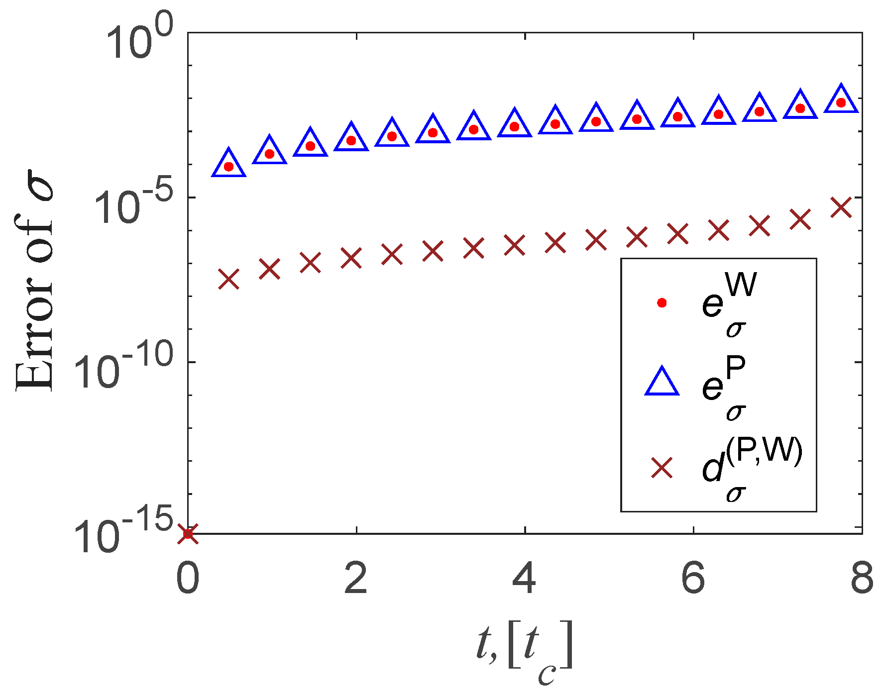
Figure 2, the
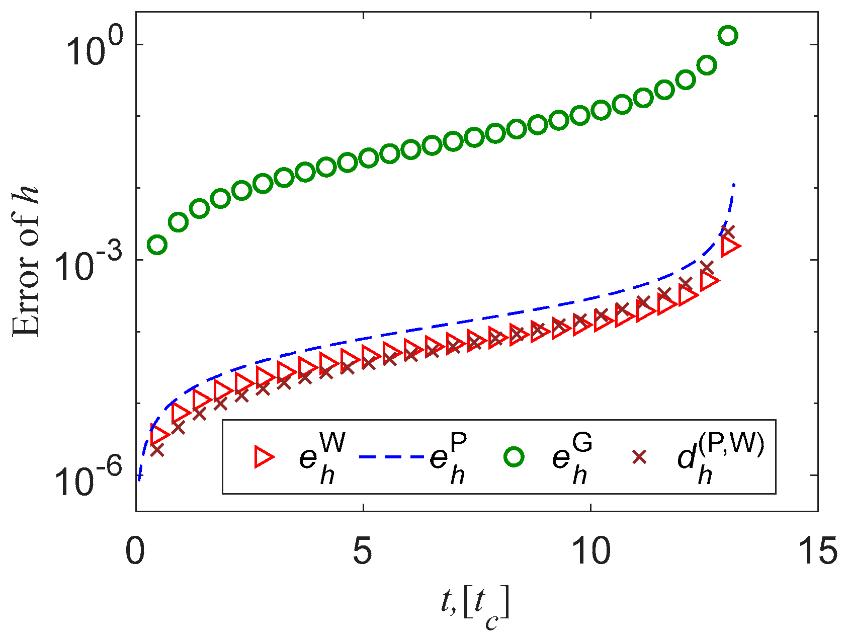
σ errors predicted by methods W and P are very close. The former has only a slight advantage over the latter. This law also holds true when predicting thickness, and the error of method G is the largest, as shown in
Figure 3.
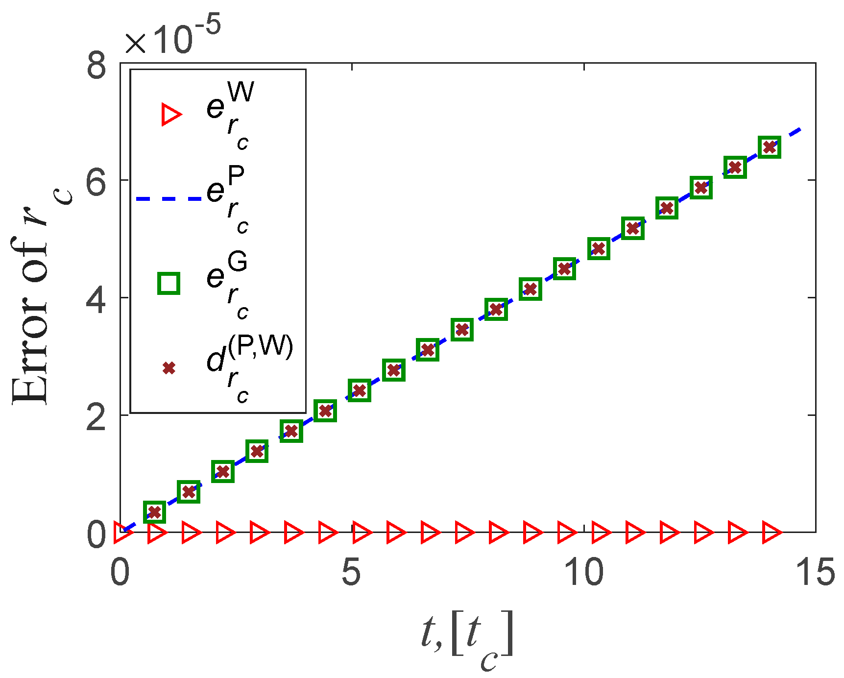
As can be seen from
Figure 4, for the value of the predicted mid-surface radius, in this time domain, the orders of magnitude of the prediction error by the three methods are all very small. Among them in this method is consistent with the reference solution best, and its accuracy is the highest.
In general, the errors of σ and (h, rc) predicted by this method and the existing two methods are all very small. Among them, the error of this method is the smallest, though its superiority is weak.
4.2. Tracking the h at Point M under the General Case
Unlike Case 1, in engineering applications such as chemical building components [
6], marine platform components [
7], etc., the more common physics phenomenon is that the internal and external corrosion intensity is rarely equal, the corrosion inhibition is functioning, and vessel itself is being not very thin. In order to research a more general model, we propose a new case with a different internal and external corrosion strengths, non-zero corrosion inhibition, and thicker geometric dimensions, see Case 2. Its results are shown in
Figure 5.
Note that, the solution expression and its calculating for thickness and radius resemble, only results for the former are delivered here for simplicity.
Case 2:
Here , , , , σ*,, , , , , , , b and can refer to the notitation list in this paper.
,, , , ], ], , ],b=0.001, , .
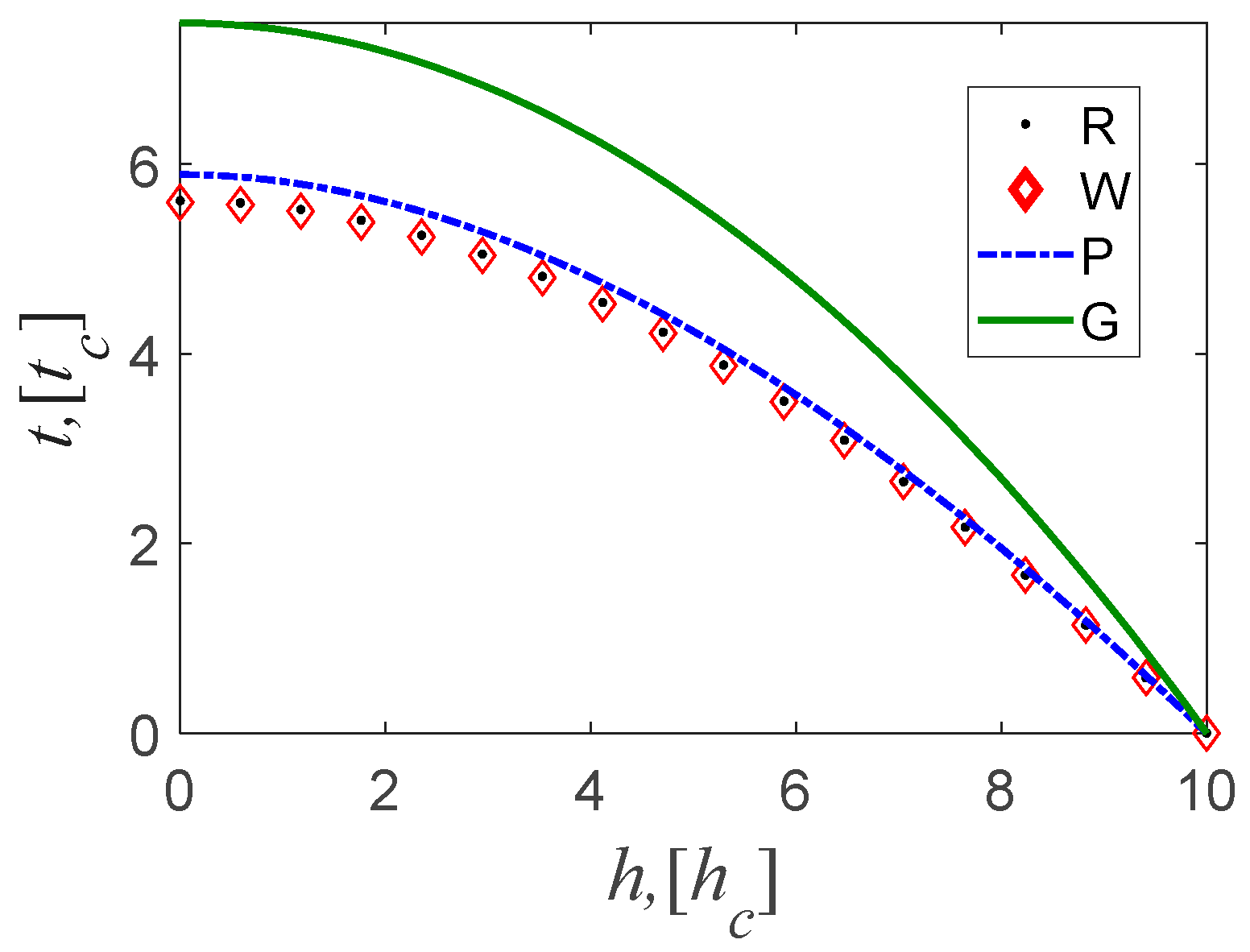
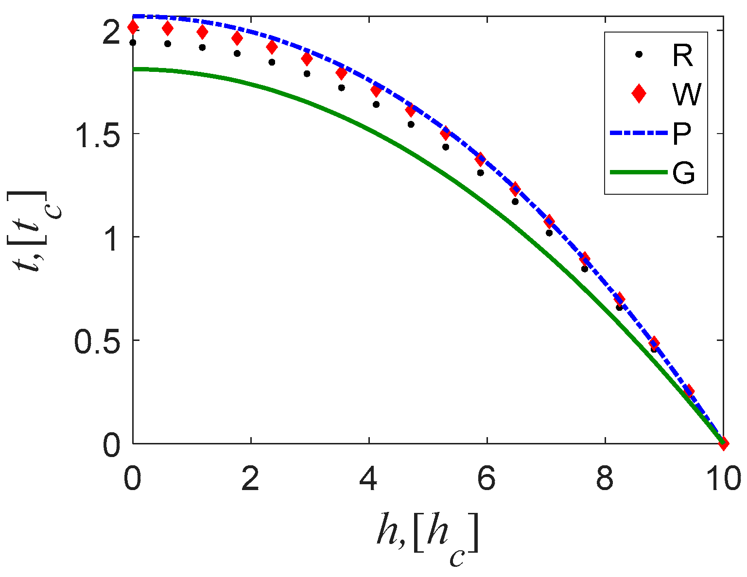
As shown in
Figure 5, the
t-
h curve predicted by our method almost coincides with the reference curve. Its accuracy is the highest, followed by [
33], and the [
27] method is the lowest.
4.3. Tracking Vessel Boundary Bi and Shape S under the General Case
For other common engineering applications, such as oil (gas) pipelines [
5] or high temperature furnace devices [
4], we seek to understand the difference of the vessel’s boundary position and shape predicted by the proposed method and other methods. With the intention of well describing this situation, we set another general example, see Case 3. Whereas, unlike Case 2, its internal corrosion intensity is higher than the external one. Corresponding results are exhibited in
Figure 6 and
Figure 7.
Case 3:
Here , , ,, , , , , b, E and can refer to the notitation list in this paper.
,, , , ], ], , ],b=0.01,, .
From
Figure 6 we note that the accuracy of tracking thickness by this method is highest. Consequently, we can quickly obtain the thickness predicted by each method at any time
tk (0<
tk<
t*); in the same way we could also obtain
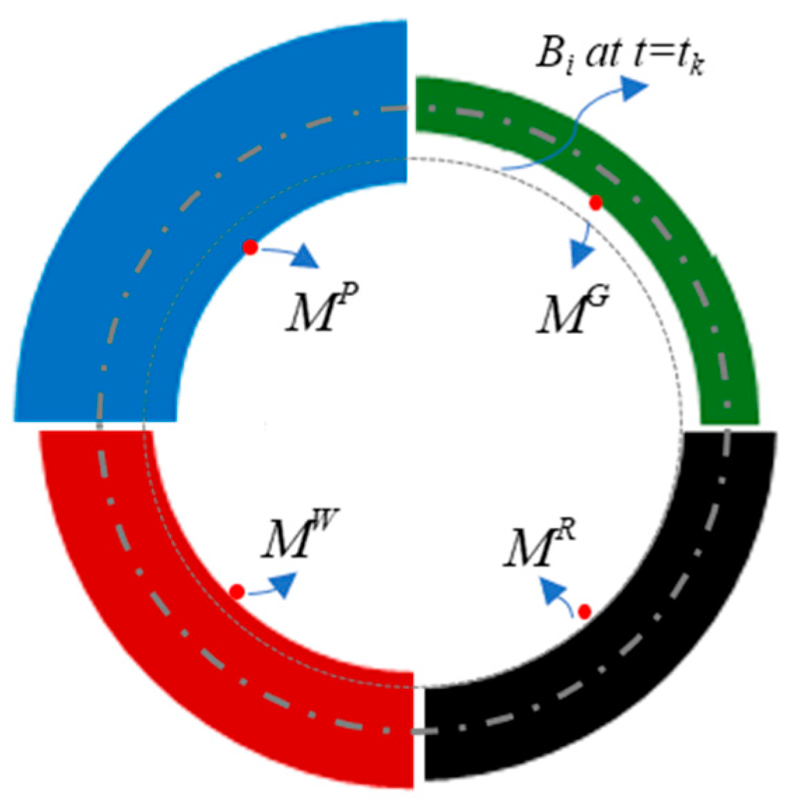
rc. Then we can qualitatively draw the position of boundary
B and the shape of shell
S at time
tk as shown in
Figure 7.
Note: Red represents results by this method; Black represents reference value by [
35]; Blue represents results by [
33]; Green represents results by [
27]).
Figure 7 shows the significant differences among the three methods in tracking M positions (
h,
rc).
MG is tracked by [
27] method. However, at
tk it is not a real boundary point, but an interior one.
MP and
MW is tracked by method in [
33] and this method respectively. However, the two positions have already dissolved and disappeared at
tk. Nevertheless, the
MW by this method is the closest to the reference value.
4.4. Predicting the Shell Critical State (t*, h*)
In some engineering applications, for example, aerial vehicles [
2], or liquid hydrogen transportation pipelines [
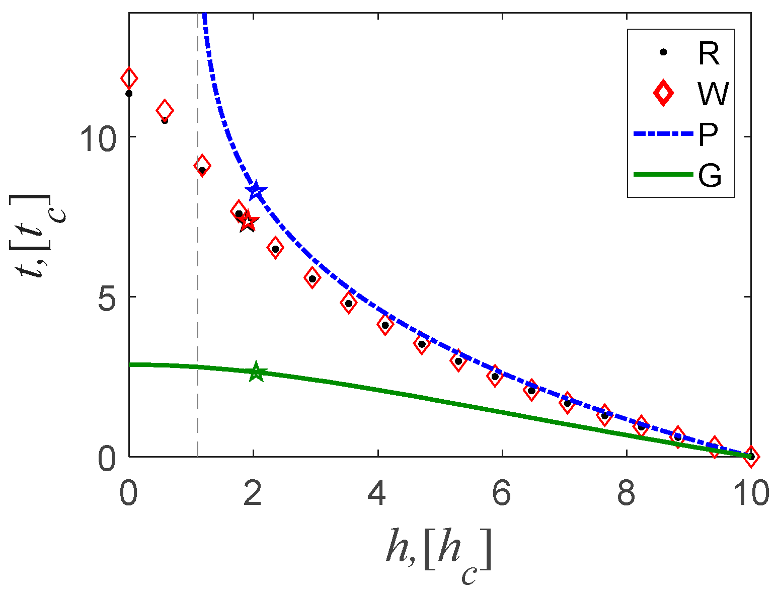
3], vessel pressure load is often relatively large, perhaps with a high corrosion inhibition, unlike case 2 and 3. It is particularly important and necessary for practitioners or operators to accurately forecast the service life of vessels in such a working condition. With this in mind, we introduce a further example as case 4. The related results are demonstrated in
Figure 8 and
Table 1.
Case 4
Here , , ,, , , , , b, E and can refer to the notitation list in this paper.
,, , , ], ], , ], ,, .
Figure 8 shows the four
h-t curves predicted by different methods. The curve of this method is almost consistent with the reference method, indicating that this method has the highest accuracy, and the higher one results from the [
33] method. The lowest level of agreement is seen from the [
27] method.
Let us note that in the curve of [
33],
t tends to positive infinity when
h approaches 1.14 [
lc]. This phenomenon shows that the shell will never completely dissolve (it has a remaining thickness of at least 1.14 [
lc] no matter how much time has passed), assuming the shell has not failed before then. This suggestion is somewhat inconsistent with physical phenomena.
Table 1 shows that the error of
t* by [
33] reaches 13%, which exceeds the general engineering accuracy (5%). Therefore, the lifetime it predicts is difficult to guarantee reliability. In contrast, the error of this method is less than 1%, which is lower than the general engineering accuracy, and its predicted lifetime is much more reliable and thus more useful. The error of
h* follows similarly.
5. Conclusions
Having described the existing research methods relating to corrosion problems in pressured vessels and discussed their evolution, advantages, and disadvantages, we justified that there is a strong need for uniform corrosion analysis methods for both current and new applications. Existing methods struggle to meet this need. Accordingly, this paper proposes an improved approach with a view to addressing current needs. This novel approach was successfully implemented. The contribution of this new method is mainly reflected in: popularizing existing methods for engineering applications, research technology for physical science, nonlinear differential equation solving methods and techniques for mathematics, etc.
5.1. Contributions to Engineering Applications
The proposed method generalizes a popular method [
33] in engineering applications, the promotion and improvement are as follows:
- (a)
Our method achieves a global, simultaneous tracking of shell shape (thickness and midplane radius) and stress. Therefore, we generalize those existing methods, which usually solve only for thickness, or only for stress.
- (b)
Moreover, relative to the existing methods, their respective analytical solutions are all: easy to program, not more time-consuming, operator-friendly, and more accurate. It is more widely applicable, functioning in settings with large-scale time domains and general working conditions.
- (c)
This general case refers to: more general corrosion conditions (internal and external corrosion rates in any ratio), pressure conditions (internal and external pressure in any ratio) or geometry (thin shell, medium-thick shell, or thick shell).
- (d)
Most importantly, we can obtain higher accuracy of lifetime t* and critical thickness h*. Note that the lifetime accuracy of the other method (P) is lower (or slightly lower) than this method in special and ordinary cases. In one of the cases, it even made a prediction that did not match the physical phenomenon (no matter how long it took, the shell could not be completely corroded). That is, in the long-term domain, its prediction of lifespan is distorted.
5.2. Contributions to Research Techniques in Physical Sciences
Taking the moving boundary problem (shell boundary/stress tracking and life prediction) as an example, this paper explores a physical science research technique that is promising to be universal. That is, how to improve the solution itself by physically improving the parameters of the solution (method) and successfully without complicating the form of the solution and the implementation of the application.
5.3. Contributions to Methods and Techniques for Solving Systems of Nonlinear Differential Equations in Mathematics
Nonlinearity is everywhere [
40] (on all time and spatial scales). Many phenomena of this nonlinear excitation naturally include the failure of general corrosion of pressure vessels [
41]. The problem is to solve its first-order nonlinear differential equation system (one independent variable, time; two dependent variables,
ri and
ro ; and two intermediate variables,
iand
o).
Analytical solutions for such a system of equations are generally not available in mathematics [42]. In general, one can only obtain its numerical solution (by simple iteration method, Newton iteration method, Newton-Raphson method, spline function, Hermite interpolation, Lagrange interpolation, etc.), or do some qualitative analysis of it (e.g., its stability study or equilibrium point analysis) [42]. If one wants to obtain its analytical solution, one must achieve the separation of dependent and independent variables within the system of equations (or equation decoupling).
To circumvent this difficulty, the P (or G) method simply separated the independent variable (t) and the dependent variable (rc) by assuming rc = rc0, thus reducing the system of equations to just one equation. An analytic solution for h could then be readily found.
Our approach is different. We first analyze the phase trajectory of the two dependent variables of this equation and obtain their explicit relationship. Then, we introduce reasonable assumptions, (e.g., ignore higher-order terms of small terms) to simplify the relationship between the two dependent variables. This simplification in turn reduces the original system of equations to one equation, which allows us to obtain its analytical solution elegantly.
During solving, this paper also proposes another mathematical technique, which is to properly introduce the intermediate variable x (x= h /rc). This distinctive introduction plays a key role in the successful separation of the original two intermediate variables (iando).
From the above, it is readily seen that by successfully solving the extremely difficult nonlinear differential equation system, we have contributed a general mathematical method (analyzing the equivalence line and obtaining the nonlinear relationship of the dependent variable) and a mathematical technique (introducing an appropriate intermediate variable, x). The successful use of both in this paper demonstrates their utility in the study of non-linear problems.
5.4. The Proposed Method Needs Further Discussion
As is the case with any new method, the proposed one needs further study, in particular if one wishes to extend it for different geometries (ellipsoidal spherical shell, cylindrical shell, etc.) or introduce further features such as temperature. The authors would suggest that one employ numerical solutions, analytical solutions, and qualitative analysis (studies of stability and equilibrium) for such a study.
Figure 1.
Characterization for shell S, boundary B and a trajectory of a point M lying at the boundary.
Figure 1.
Characterization for shell S, boundary B and a trajectory of a point M lying at the boundary.
Figure 2.
Stress error (difference) between methods ,and
Figure 2.
Stress error (difference) between methods ,and
Figure 3.
Thickness error (difference) between methods ,,and.
Figure 3.
Thickness error (difference) between methods ,,and.
Figure 4.
Mid-surface radius error (difference) between methods ,,and
Figure 4.
Mid-surface radius error (difference) between methods ,,and
Figure 5.
h-t curves traced by R, W, P, and G method.
Figure 5.
h-t curves traced by R, W, P, and G method.
Figure 6.
h-t curves traced by P,W,P, and G method.
Figure 6.
h-t curves traced by P,W,P, and G method.
Figure 7.
Qualitative geometric shape of S, Bi and M.
Figure 7.
Qualitative geometric shape of S, Bi and M.
Figure 8.
h-t curves and their t*, h* traced by R,W,P,and G method.
Figure 8.
h-t curves and their t*, h* traced by R,W,P,and G method.
Table 1.
t* error (difference) between methods ,,and (%) (j=W,P,G).
Table 1.
t* error (difference) between methods ,,and (%) (j=W,P,G).
|
or |
|
|
|
|
| Value |
0.6 |
13.3 |
70.0 |
12.7 |
|
or |
|
|
|
|
| Value |
0.8 |
7.6 |
7.6 |
6.8 |

