Galilean Non-invariance of Maxwell Equations Revisited

1. Introduction

The realization that Maxwell equations are not invariant under the Galilean transformation is credited to H. A. Lorentz who in his landmark paper [1] published in 1904, among other important findings, reported that Maxwell equations are not Galilei invariant. This important finding motivated Lorentz to discover the new kind of coordinate transformation between inertial coordinate systems under which the Maxwell equations remain invariant.

The reason why Lorentz was seeking for this new transformation lies in the principle of relativity which states that the physical laws must remain the same for all observers in inertial reference frames. This principle has roots in the works of Galileo Galilei, who in 1632 [2] realized that the mechanical experiments performed on a ship moving with constant velocity must yield the same results as the same mechanical experiments performed on the shore [3].

Because Lorentz believed that the Maxwell equations were not invariant under the Galilean transformation, Lorentz thought that if the Maxwell equations are to obey the principle of relativity he must then find the transformation of coordinates under which the Maxwell equations remain invariant. Lorentz indeed derived this new transformation, which is now known as the Lorentz transformation. The Lorentz transformation was later physically interpreted by Einstein who formulated the theory of special relativity [4], and the Lorentz transformation was in accordance with Einstein’s theory.

Therefore, the importance of Lorentz’s conclusion that Maxwell equations are not invariant under the Galilean transformation cannot be understated. Thus, it is important to examine how Lorentz arrived to this conclusion. Although Lorentz did not explicitly write this, Lorentz realized that the time derivative under the Galilean transformation transforms as:

$$\frac{\partial }{\partial t}=\frac{\partial }{\partial t^{\prime }}-v\frac{\partial }{\partial x^{\prime }}$$

(1)

By applying the Equation (1) to Faraday’s law, and to Maxwell-Ampere law, Lorentz obtained the Galilean transformation of these two laws as:

$$\begin{array}{cc}\hfill {\nabla }^{\prime }\times {\overrightarrow{E}}^{\prime }=& -\left(\frac{\partial }{\partial t^{\prime }}-v\frac{\partial }{\partial x^{\prime }}\right){\overrightarrow{B}}^{\prime }\hfill \end{array}$$

(2)

$$\begin{array}{cc}\hfill {\nabla }^{\prime }\times {\overrightarrow{B}}^{\prime }=& \mu {\overrightarrow{J}}^{\prime }+\frac{1}{c^2}\left(\frac{\partial }{\partial t^{\prime }}-v\frac{\partial }{\partial x^{\prime }}\right){\overrightarrow{E}}^{\prime }\hfill \end{array}$$

(3)

From the equations above, Lorentz concluded that the Maxwell equations are not invariant in the mathematical form under the Galilean transformation. This convinced Lorentz that the Galilean transformation is not physical. Furthermore, Lorentz’s conclusion about Galilean non-invariance of Maxwell equations was later confirmed by many subsequent researchers [5,6,7,8,9].

However, as shown in the Section 5 of this paper, the Galilean transformation of the time derivative $\frac{\partial }{\partial t}$ is not always given by the Equation (1). This is because, as shown in Section 5, the Galilean transformation of $\frac{\partial }{\partial t}$ is function dependent. Moreover, it was also shown in the Section 5 that if the electric field $\overrightarrow{E}$ and the magnetic field $\overrightarrow{B}$ are the function of the coordinates of both an observer and the source then the transformation given by the Equation (1) is obtained when one applies the Galilean transformation to the coordinates of an observer and forgets to apply the Galilean transformation to the coordinates of the source. In short, it is demonstrated that Lorentz and subsequent researchers used incorrect mathematical procedure to demonstrate Galilean non-invariance of Maxwell equations.

In fact, it is also demonstrated in the Section 5 that the only correct way to prove that the Maxwell equations are not invariant under the Galilean transformation is to prove that any of the following twenty four equations are not valid:

$$\begin{array}{c}\hfill \frac{\partial }{\partial x_i}\overrightarrow{E}=\frac{\partial }{\partial x_i^{\prime }}{\overrightarrow{E}}^{\prime }\end{array}$$

(4)

$$\begin{array}{c}\hfill \frac{\partial }{\partial x_i}\overrightarrow{B}=\frac{\partial }{\partial x_i^{\prime }}{\overrightarrow{B}}^{\prime }\end{array}$$

(5)

where $x_i\in \{x,y,z,t\}$ and $x_i^{\prime }\in \{x^{\prime },y^{\prime },z^{\prime },t^{\prime }\}$. The reason why the equations (4) and (5) are in fact twenty four equations is because the vectors $\overrightarrow{E}$ and $\overrightarrow{B}$ each have three Cartesian components and there are four derivatives for each component.

If one is to use the equations (4) and (5) to prove Galilean invariance, or Galilean non-invariance, of Maxwell equations then one needs to know the exact mathematical form of the electric field $\overrightarrow{E}$ and the magnetic field $\overrightarrow{B}$ in advance. For that reason, the Liénard-Wiechert electric and magnetic fields were selected in order to prove or to disprove the Galilean invariance of Maxwell equations. This is because Liénard-Wiechert electromagnetic field are the only known closed-form solutions for the electromagnetic fields of a single charge in arbitrary motion.

As shown in the Section 4 of this paper, it is evident that the Maxwell equations, when applied to Liénard-Wiechert electromagnetic fields, are invariant under the Galilean transformation. From here, one can only arrive to conclusion that Lorentz’s conclusion about Galilean non-invariance of Maxwell equations is the result of a mathematical error, and that Maxwell equations are indeed invariant under the Galilean transformation.

2. The Maxwell Equations and the Liénard-Wiechert potentials

Maxwell equations that describe the electric and magnetic fields caused by electric charges and currents are considered one of the greatest achievements of theoretical physics. In modern times the original Maxwell equations are written in concise mathematical form as the set of four Maxwell equations governing the laws of electrodynamics:

$$\begin{array}{cc}\hfill \nabla ·\overrightarrow{D}=& \rho \hfill \end{array}$$

(6)

$$\begin{array}{cc}\hfill \nabla ·\overrightarrow{B}=& 0\hfill \end{array}$$

(7)

$$\begin{array}{cc}\hfill \nabla \times \overrightarrow{E}=& -\frac{\partial \overrightarrow{B}}{\partial t}\hfill \end{array}$$

(8)

$$\begin{array}{cc}\hfill \nabla \times \overrightarrow{B}=& \mu \overrightarrow{J}+\frac{1}{c^2}\frac{\partial \overrightarrow{E}}{\partial t}\hfill \end{array}$$

(9)

where $\overrightarrow{E}$ is the magnetic field, and $\overrightarrow{B}$ is the magnetic field. The electric and magnetic field can be expressed as the functions of scalar electric potential $\varphi$ and the magnetic vector potential $\overrightarrow{A}$ as:

$$\begin{array}{cc}\hfill \overrightarrow{E}=& -\nabla \varphi -\frac{\partial \overrightarrow{A}}{\partial t}\hfill \end{array}$$

(10)

$$\begin{array}{cc}\hfill \overrightarrow{B}=& \nabla \times \overrightarrow{A}\hfill \end{array}$$

(11)

The closed-form solutions to Maxwell equations are rare, however, there exists the closed form solution to Maxwell equations for the electric and magnetic fields caused by the single moving charge. If the electric and magnetic field are caused by the single moving point charge then the potentials $\varphi$ and $\overrightarrow{A}$ become the retarded in time Liénard-Wiechert potentials [10,11] given as:

$$\begin{array}{cc}\hfill \varphi =\varphi (\overrightarrow{r},t)=& \frac{1}{4\pi ϵ}\frac{q}{\left(1-{\overrightarrow{\beta }}_s·{\overrightarrow{n}}_s\right)\left|\overrightarrow{r}-{\overrightarrow{r}}_s\right|}\hfill \end{array}$$

(12)

$$\begin{array}{cc}\hfill \overrightarrow{A}=\overrightarrow{A}(\overrightarrow{r},t)=& \frac{{\overrightarrow{\beta }}_s}{c}\varphi \hfill \end{array}$$

(13)

where vector ${\overrightarrow{r}}_s$ represents the location of the moving source charge at retarded time $t_r$:

$${\overrightarrow{r}}_s={\overrightarrow{r}}_s\left(t_r\right)=\left\{x_s\left(t_r\right),y_s\left(t_r\right),z_s\left(t_r\right)\right\}$$

(14)

and where vector $\overrightarrow{r}$ represents the location of fixed observer:

$$\overrightarrow{r}=\left\{x,y,z\right\}$$

(15)

The vector ${\overrightarrow{\beta }}_s$ represents the velocity of the source charge at retarded time $t_r$ divided by the speed of light c, and it is commonly given in the scientific literature as:

$${\overrightarrow{\beta }}_s={\overrightarrow{\beta }}_s\left(t_r\right)=\frac{1}{c}\frac{d}{dt}{\overrightarrow{v}}_s\left(t_r\right)=\frac{1}{c}\frac{d}{dt}{\overrightarrow{r}}_s\left(t_r\right)$$

(16)

where ${\overrightarrow{v}}_s\left(t_r\right)$ is the velocity of the source. The reason why it is emphasized that the vector ${\overrightarrow{\beta }}_s$ is commonly given in the literature as the Equation (16) lies in the fact that, as shown in the Section 3 of this paper, the mathematical representation of the vector ${\overrightarrow{\beta }}_s$ given by the Equation (16) is not the best possible representation of the vector ${\overrightarrow{\beta }}_s$.

The vector ${\overrightarrow{n}}_s$ is an unit vector pointing from the location of the source charge at the time $t_r$ to the location of the observer:

$${\overrightarrow{n}}_s={\overrightarrow{n}}_s(t,t_r)=\frac{\overrightarrow{r}-{\overrightarrow{r}}_s\left(t_r\right)}{\left|\overrightarrow{r}-{\overrightarrow{r}}_s\left(t_r\right)\right|}$$

(17)

One may now note that the potentials $\varphi$ and $\overrightarrow{A}$ are the functions of the time t and not of the retarded time $t_r$. This is because the time t is the time when the electric and magnetic fields emitted by the source charge at time $t_r$ propagates to the observer located at position $\overrightarrow{r}$. In fact, the time t and the retarded time $t_r$ are related by the following equation:

$$t=t_r+\frac{\left|\overrightarrow{r}-{\overrightarrow{r}}_s\left(t_r\right)\right|}{c}$$

(18)

and the retarded time $t_r$ is the solution to the Equation (18). Although it may be very difficult to solve the Equation (18) for retarded time $t_r$, it is clear that the retarded time $t_r$ is the function of variables x, y, z and t, and for this reason it may be written:

$$t_r=t_r(x,y,z,t)$$

(19)

Hence, the electric and magnetic fields $\overrightarrow{E}$ and $\overrightarrow{B}$ are indeed the functions of the time t because the retarded time is the function of the time t.

The electric field $\overrightarrow{E}$ and the magnetic field $\overrightarrow{B}$ are calculated by substituting the Liénard-Wiechert potentials $\varphi$ and $\overrightarrow{A}$ into the equations (10) and (11) which yields:

$$\begin{array}{cc}\hfill \overrightarrow{E}(\overrightarrow{r},t)=& \frac{1}{4\pi ϵ}\left(\frac{q\left({\overrightarrow{n}}_s-{\overrightarrow{\beta }}_s\right)}{{\gamma }^2{\left(1-{\overrightarrow{n}}_s·{\overrightarrow{\beta }}_s\right)}^3{\left|\overrightarrow{r}-{\overrightarrow{r}}_s\right|}^2}+\frac{q{\overrightarrow{n}}_s\times \left(\left({\overrightarrow{n}}_s-{\overrightarrow{\beta }}_s\right)\times {\dot{\overrightarrow{\beta }}}_s\right)}{c{\left(1-{\overrightarrow{n}}_s·{\overrightarrow{\beta }}_s\right)}^3\left|\overrightarrow{r}-{\overrightarrow{r}}_s\right|}\right)\hfill \end{array}$$

(20)

$$\begin{array}{cc}\hfill \overrightarrow{B}(\overrightarrow{r},t)=& \frac{{\overrightarrow{n}}_s}{c}\times \overrightarrow{E}(\overrightarrow{r},t)\hfill \end{array}$$

(21)

where ${\dot{\overrightarrow{\beta }}}_s$ is the acceleration of the source at time $t_r$ divided by the speed of light:

$${\dot{\overrightarrow{\beta }}}_s=\frac{1}{c}\frac{d}{dt}{\overrightarrow{v}}_s\left(t_r\right)=\frac{1}{c}\frac{d^2}{d{t}_r^2}{\overrightarrow{r}}_s\left(t_r\right)$$

(22)

and the function $\gamma$ is given by:

$$\gamma =\frac{1}{\sqrt{1-{\overrightarrow{\beta }}_s·{\overrightarrow{\beta }}_s}}$$

(23)

The equations (20) and (21) are nowadays considered the standard expressions for time retarded Liénard-Wiechert electric and magnetic fields [5,12,13] and are widely used for advanced electromagnetic calculations such as synchrotron, undulator and radar radiation [14,15,16] and in high-energy particle physics [17,18].

2.1. Some subtleties regarding the Liénard-Wiechert electromagnetic fields

Many of the subtleties regarding the Liénard-Wiechert electromagnetic fields are both explicitly and implicitly clarified in the paper about Liénard-Wiechert fields written by the author of this text [19]. For example, the charge density $\rho$ in the first Maxwell equation becomes [19]:

$$\rho =\rho (\overrightarrow{r},t)=q\delta \left(\overrightarrow{r}-{\overrightarrow{r}}_s\left(t\right)\right)$$

(24)

when the Liénard-Wiechert electric field is substituted in the Equation (6).

The current density $\overrightarrow{J}$, when the Liénard-Wiechert electromagnetic fields are substituted into the Equation (9) becomes [19]:

$$\overrightarrow{J}=\overrightarrow{J}(\overrightarrow{r},t)=q{\overrightarrow{v}}_s\left(t\right)\delta \left(\overrightarrow{r}-{\overrightarrow{r}}_s\left(t\right)\right)$$

(25)

where ${\overrightarrow{v}}_s\left(t\right)$ is the velocity of the source at time t.

Furthermore, from the Appendix C.1 of the cited paper [19], specifically from the equation (A42) of that paper, it is evident that the velocity of the source ${\overrightarrow{v}}_s\left(t\right)$ can be written as:

$${\overrightarrow{v}}_s\left(t\right)=-\frac{\partial }{\partial t}\left(\overrightarrow{r}-{\overrightarrow{r}}_s\left(t\right)\right)$$

(26)

If the position vector $\overrightarrow{r}$ of the observer is fixed (constant) then the equation (26) reduces to:

$${\overrightarrow{v}}_s\left(t\right)=\frac{\partial }{\partial t_r}{\overrightarrow{r}}_s\left(t\right)$$

(27)

However, if the position vector $\overrightarrow{r}$ is not fixed, such as when transformed by Galilean transformation, then the Equation (26) must be considered as the correct equation, and the Equation (27) can no longer be considered correct.

On the final note, in order to calculate the derivatives of the electric field $\overrightarrow{E}(\overrightarrow{r},t)$ and the magnetic field $\overrightarrow{B}(\overrightarrow{r},t)$ with respect to variables x, y, z and t it is necessary to calculate the derivatives of the function $t_r=t_r(x,y,z,t)$ with respect to these variables. By differentiating the Equation (18) with respect to time t one obtains:

$$\frac{\partial t_r}{\partial t}=\frac{1}{1-\overrightarrow{{\beta }_s}·{\overrightarrow{n}}_s}$$

(28)

Furthermore, differentiating the Equation (19) with respect to variables x, y and z yields:

$$\frac{\partial t_r}{\partial x_i}=-\frac{1}{c}\frac{n_{s_i}}{1-{\overrightarrow{\beta }}_s·{\overrightarrow{n}}_s}$$

(29)

where $x_i\in \{x,y,z\}$ and $n_{s_i}\in \{n_{s_x},n_{s_y},n_{s_z}\}$, and where $n_{s_x}$, $n_{s_y}$ and $n_{s_z}$ are the Cartesian components of the vector ${\overrightarrow{n}}_s$.

3. Galilean transformation of Liénard-Wiechert electric and magnetic field

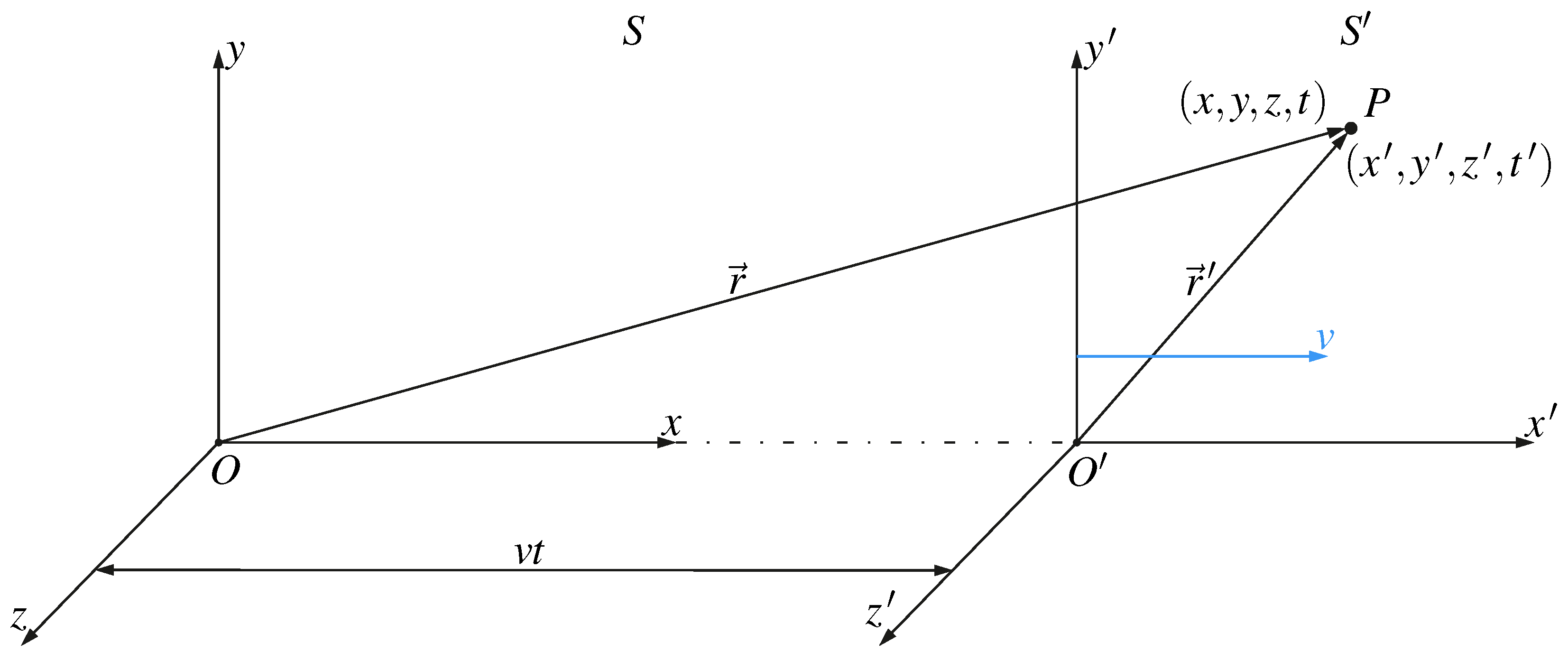
In this section, the Liénard-Wiechert electric and magnetic fields are transformed from the coordinate system S to the coordinate system $S^{\prime }$, both of which are shown in the Figure 1. The coordinate system $S^{\prime }$ moves along x axis of the coordinate system S with constant velocity v. In the coordinate system S the point P is located at coordinates $\{x,y,z\}$ and the variables x, y and z do not change with time. In the coordinate system $S^{\prime }$, the same point P is described by the coordinates $\{x^{\prime },y^{\prime },z^{\prime }\}$, and the coordinate $x^{\prime }$ is the function of the time. The coordinates of the point P in $S^{\prime }$ are related to the coordinates of the point P in S via the following transformation:

$$\begin{array}{cc}\hfill x^{\prime }=& x-vt\hfill \end{array}$$

(30)

$$\begin{array}{cc}\hfill y^{\prime }=& y\hfill \end{array}$$

(31)

$$\begin{array}{cc}\hfill z^{\prime }=& z\hfill \end{array}$$

(32)

$$\begin{array}{cc}\hfill t^{\prime }=& t\hfill \end{array}$$

(33)

The equations above are collectively known as the Galilean transformation which transforms the coordinates from the coordinate system S to the coordinate system $S^{\prime }$.

Furthermore, from the equations (30) - (33) it follows that there exists an inverse Galilean transformation which transforms the coordinates from the coordinate system $S^{\prime }$ to the coordinate system S:

$$\begin{array}{cc}\hfill x=& x^{\prime }+v{t}^{\prime }\hfill \end{array}$$

(34)

$$\begin{array}{cc}\hfill y=& y^{\prime }\hfill \end{array}$$

(35)

$$\begin{array}{cc}\hfill z=& z^{\prime }\hfill \end{array}$$

(36)

$$\begin{array}{cc}\hfill t=& t^{\prime }\hfill \end{array}$$

(37)

Because the aim of this section is to transform the Liénard-Wiechert electric and magnetic field from coordinate system S to coordinate system $S^{\prime }$ we start by transforming the vector $\overrightarrow{r}=\{x,y,z\}$ from the coordinate system S to the coordinate system $S^{\prime }$. This transformation can be achieved by the application of the inverse Galilean transformation to the vector $\overrightarrow{r}$:

$$\overrightarrow{r}=\left\{x,y,z\right\}=\left\{x^{\prime }+v{t}^{\prime },y^{\prime },z^{\prime }\right\}={\overrightarrow{r}}^{\prime }+\left\{v{t}^{\prime },0,0\right\}$$

(38)

where the vector ${\overrightarrow{r}}^{\prime }=\left\{x^{\prime },y^{\prime },z^{\prime }\right\}$.

Because of the Galilean transformation the retarded time $t_r$ in S is equal to the retarded time $t_r^{\prime }$ in $S^{\prime }$, i.e. $t_r=t_r^{\prime }$. Then, the application of the inverse Galilean transformation to the vector ${\overrightarrow{r}}_s\left(t_r\right)$ yields:

$$\begin{array}{cc}\hfill {\overrightarrow{r}}_s\left(t_r\right)=& \left\{x_s\left(t_r\right),y_s\left(t_r\right),z_s\left(t_r\right)\right\}=\left\{x_s^{\prime }\left(t_r^{\prime }\right)+v{t}^{\prime },y_s^{\prime }\left(t_r^{\prime }\right),z_s^{\prime }\left(t_r^{\prime }\right)\right\}=\hfill \\ \hfill =& {\overrightarrow{r}}_s^{\prime }\left(t_r^{\prime }\right)+\left\{v{t}^{\prime },0,0\right\}\hfill \end{array}$$

(39)

where the vector ${\overrightarrow{r}}_s^{\prime }\left(t_r^{\prime }\right)=\left\{x_s^{\prime }\left(t_r^{\prime }\right),y_s^{\prime }\left(t_r^{\prime }\right),z_s^{\prime }\left(t_r^{\prime }\right)\right\}$ represents the position vector of the source viewed from the coordinate system $S^{\prime }$ at the time $t^{\prime }=t$.

Using the equations (38) and (39) it is now possible to convert the difference of vectors $\overrightarrow{r}$ and ${\overrightarrow{r}}_s\left(t_r\right)$ from the coordinate system S to the coordinate system $S^{\prime }$ as:

$$\overrightarrow{r}-{\overrightarrow{r}}_s\left(t_r\right)={\overrightarrow{r}}^{\prime }+\left\{v{t}^{\prime },0,0\right\}-\left({\overrightarrow{r}}_s^{\prime }\left(t_r^{\prime }\right)+\left\{v{t}^{\prime },0,0\right\}\right)={\overrightarrow{r}}^{\prime }-{\overrightarrow{r}}_s^{\prime }\left(t_r^{\prime }\right)$$

(40)

The equation above means that the distance between the source and an observer in the coordinate system $S^{\prime }$ is the same as in coordinate system S regardless of the time $t=t^{\prime }$ and regardless of the velocity v.

Using the Equation (40) the vector ${\overrightarrow{n}}_s$ in the coordinate system S can be transformed to the coordinate system $S^{\prime }$. By substituting the Equation (40) into the Equation (17) it is obtained:

$${\overrightarrow{n}}_s=\frac{\overrightarrow{r}-{\overrightarrow{r}}_s\left(t_r\right)}{\left|\overrightarrow{r}-{\overrightarrow{r}}_s\left(t_r\right)\right|}=\frac{{\overrightarrow{r}}^{\prime }-{\overrightarrow{r}}_s^{\prime }\left(t_r^{\prime }\right)}{\left|{\overrightarrow{r}}^{\prime }-{\overrightarrow{r}}_s^{\prime }\left(t_r^{\prime }\right)\right|}$$

(41)

The vector ${\overrightarrow{n}}_s$ in the coordinate system S represents an unit vector pointing from the location of the source at retarded time $t_r$ to the location of observer. In the coordinate system $S^{\prime }$, one can define the vector ${\overrightarrow{n}}_s^{\prime }$ that has the same meaning:

$${\overrightarrow{n}}_s^{\prime }=\frac{{\overrightarrow{r}}^{\prime }-{\overrightarrow{r}}_s^{\prime }\left(t_r^{\prime }\right)}{\left|{\overrightarrow{r}}^{\prime }-{\overrightarrow{r}}_s^{\prime }\left(t_r^{\prime }\right)\right|}$$

(42)

By comparison of the right hand sides of the equations (41) and (42) it follows that:

$${\overrightarrow{n}}_s={\overrightarrow{n}}_s^{\prime }$$

(43)

We now arrive to the critical part of the transformation of Liénard-Wiechert electric and magnetic field from the coordinate system S to the coordinate system $S^{\prime }$. The problem here is that the vector ${\overrightarrow{\beta }}_s\left(t_r\right)$ in the coordinate system S, given by the Equation (16), can be defined in at least two ways that are numerically identical in the coordinate system S:

$$\begin{array}{cc}\hfill {\overrightarrow{\beta }}_s\left(t_r\right)=& \frac{1}{c}\frac{d}{d{t}_r}{\overrightarrow{r}}_s\left(t_r\right)\hfill \end{array}$$

(44)

$$\begin{array}{cc}\hfill {\overrightarrow{\beta }}_s\left(t_r\right)=& -\frac{1}{c}\frac{d}{d{t}_r}\left[\overrightarrow{r}-{\overrightarrow{r}}_s\left(t_r\right)\right]\hfill \end{array}$$

(45)

Although the equations (44) and (45) produce numerically identical results in S, the expressions (44) and (45) are not mathematically identical expressions. Furthermore, when the expressions (44) and (45) are converted to the coordinate system $S^{\prime }$ using the inverse Galilean transformation, these expressions do not yield numerically identical results in $S^{\prime }$. For that reason it is crucial to select the correct mathematical representation of the vector ${\overrightarrow{\beta }}_s\left(t_r\right)$.

If one desires to find the correct mathematical expression for the vector ${\overrightarrow{\beta }}_s$ one must look at how the Liénard-Wiechert potentials are derived. The scalar Liénard-Wiechert potential $\varphi$ is the solution to the following inhomogeneous three dimensional wave equation:

$${\nabla }^2\varphi -\frac{1}{c^2}\frac{{\partial }^2\varphi }{\partial t^2}=\frac{q}{ϵ}\delta \left(\overrightarrow{r}-{\overrightarrow{r}}_s\left(t\right)\right)$$

(46)

where $\delta \left(\overrightarrow{r}-{\overrightarrow{r}}_s\left(t\right)\right)$ is three dimensional Dirac delta function. Using the Green’s function method [20] it follows that the solution to the equation above is:

$$\varphi =\frac{q}{ϵ}\int d{V}^{\prime }\int d{t}^{\prime }\delta \left({\overrightarrow{r}}^{\prime }-{\overrightarrow{r}}_s\left(t^{\prime }\right)\right)G({\overrightarrow{r}}^{\prime },t^{\prime };\overrightarrow{r},t)$$

(47)

where the function $G({\overrightarrow{r}}^{\prime },t^{\prime };\overrightarrow{r},t)$ is the free space Green’s function for three dimensional wave equation given by [21]:

$$G({\overrightarrow{r}}^{\prime },t^{\prime };\overrightarrow{r},t)=\frac{\delta \left(t-t^{\prime }-\frac{\left|\overrightarrow{r}-{\overrightarrow{r}}^{\prime }\right|}{c}\right)}{4\pi \left|\overrightarrow{r}-{\overrightarrow{r}}^{\prime }\right|}$$

(48)

Substituting the Equation (48) into the Equation (47) yields:

$$\varphi =\frac{q}{ϵ}\int d{V}^{\prime }\int d{t}^{\prime }\delta \left({\overrightarrow{r}}^{\prime }-{\overrightarrow{r}}_s\left(t^{\prime }\right)\right)\frac{\delta \left(t-t^{\prime }-\frac{\left|\overrightarrow{r}-{\overrightarrow{r}}^{\prime }\right|}{c}\right)}{4\pi \left|\overrightarrow{r}-{\overrightarrow{r}}^{\prime }\right|}$$

(49)

If we first integrate over whole space $V^{\prime }$, the Dirac delta function $\delta \left({\overrightarrow{r}}^{\prime }-{\overrightarrow{r}}_s\left(t^{\prime }\right)\right)$ selects the point ${\overrightarrow{r}}^{\prime }={\overrightarrow{r}}_s\left(t^{\prime }\right)$, thus, the equation above becomes:

$$\varphi =\frac{q}{ϵ}\int d{t}^{\prime }\frac{\delta \left(t-t^{\prime }-\frac{\left|\overrightarrow{r}-{\overrightarrow{r}}_s\left(t^{\prime }\right)\right|}{c}\right)}{4\pi \left|\overrightarrow{r}-{\overrightarrow{r}}_s\left(t^{\prime }\right)\right|}$$

(50)

To proceed, we now make use of the following identity involving Dirac delta function [22,23]:

$$\delta \left(f\left(u\right)\right)=\frac{\delta \left(u-u_0\right)}{{\left|\frac{d}{du}f\left(u\right)\right|}_{u=u_0}}$$

(51)

where $u_0$ is the solution to the equation $f\left(u_0\right)=0$. Note that the following equation is equal to zero:

$$t-t^{\prime }-\frac{\left|\overrightarrow{r}-{\overrightarrow{r}}_s\left(t^{\prime }\right)\right|}{c}=0$$

(52)

only if $t^{\prime }=t_0^{\prime }=t_r$, which is clear from the Equation (18). Then, by the application of the identity (51) to Dirac delta function in the Equation (50) one obtains:

$$\begin{array}{cc}\hfill \delta \left(t-t^{\prime }-\frac{\left|\overrightarrow{r}-{\overrightarrow{r}}_s\left(t^{\prime }\right)\right|}{c}\right)=& \frac{\delta \left(t^{\prime }-t_0^{\prime }\right)}{{\left|-1-\frac{\left(\overrightarrow{r}-{\overrightarrow{r}}_s\left(t^{\prime }\right)\right)·\frac{d}{d{t}^{\prime }}\left(\overrightarrow{r}-{\overrightarrow{r}}_s\left(t^{\prime }\right)\right)}{c\left|\overrightarrow{r}-{\overrightarrow{r}}_s\left(t^{\prime }\right)\right|}\right|}_{t^{\prime }=t_0^{\prime }=t_r}}\hfill \\ \hfill =& \frac{\delta \left(t^{\prime }-t_r\right)}{\left|-1+\frac{\left(\overrightarrow{r}-{\overrightarrow{r}}_s\left(t_r\right)\right)·\frac{d}{d{t}_r}\left[-\left(\overrightarrow{r}-{\overrightarrow{r}}_s\left(t_r\right)\right)\right]}{c\left|\overrightarrow{r}-{\overrightarrow{r}}_s\left(t_r\right)\right|}\right|}=\hfill \\ \hfill =& \frac{\delta \left(t^{\prime }-t_r\right)}{1-{\overrightarrow{n}}_s·\frac{1}{c}\frac{d}{d{t}_r}\left[-\left(\overrightarrow{r}-{\overrightarrow{r}}_s\left(t_r\right)\right)\right]}\hfill \end{array}$$

(53)

Substituting the Equation (53) into the Equation (50) yields the Liénard-Wiechert scalar potential:

$$\begin{array}{cc}\hfill \varphi =& \frac{q}{ϵ}\int d{t}^{\prime }\frac{\delta \left(t^{\prime }-t_r\right)}{4\pi \left(1-{\overrightarrow{n}}_s·\frac{1}{c}\frac{d}{d{t}_r}\left[-\left(\overrightarrow{r}-{\overrightarrow{r}}_s\left(t_r\right)\right)\right]\right)\left|\overrightarrow{r}-{\overrightarrow{r}}_s\left(t^{\prime }\right)\right|}=\hfill \\ \hfill =& \frac{q}{4\pi ϵ}\frac{1}{\left(1-{\overrightarrow{n}}_s·{\overrightarrow{\beta }}_s\right)\left|\overrightarrow{r}-{\overrightarrow{r}}_s\left(t_r\right)\right|}\hfill \end{array}$$

(54)

where the vector ${\overrightarrow{\beta }}_s$ is:

$${\overrightarrow{\beta }}_s=\frac{1}{c}\frac{d}{d{t}_r}\left[-\left(\overrightarrow{r}-{\overrightarrow{r}}_s\left(t_r\right)\right)\right]$$

(55)

In the coordinate system S the position vector $\overrightarrow{r}$ is not the function of time, and because of this $\frac{d\overrightarrow{r}}{dt}=0$ in S. Therefore, in the coordinate system S the following equation holds:

$${\overrightarrow{\beta }}_s=\frac{1}{c}\frac{d}{d{t}_r}\left[-\left(\overrightarrow{r}-{\overrightarrow{r}}_s\left(t_r\right)\right)\right]=\frac{1}{c}\frac{d}{d{t}_r}{\overrightarrow{r}}_s\left(t_r\right)$$

(56)

However, the equations (55) and (56) give different results when Galilei transformed to the coordinate system $S^{\prime }$ which means that Equation (56) is valid only in the coordinate system S. Therefore, although the Equation (56) holds in S, it is clear that the vector ${\overrightarrow{\beta }}_s$ is generally given by the Equation (55) and not by the Equation (56).

Let us now define the vector ${\overrightarrow{\beta }}_s^{\prime }$ in the coordinate system $S^{\prime }$. According to the Equation (55) the vector ${\overrightarrow{\beta }}_s$ is the derivative with respect to retarded time of the difference between the position vector of the source at time $t_r$ and the position vector of the observer $\overrightarrow{r}$ divided by c. In the coordinate system $S^{\prime }$ we can define the vector ${\overrightarrow{\beta }}_s^{\prime }$ in $S^{\prime }$ that has the same meaning:

$${\overrightarrow{\beta }}_s^{\prime }=\frac{1}{c}\frac{d}{d{t}_r^{\prime }}\left[-\left({\overrightarrow{r}}^{\prime }-{\overrightarrow{r}}_s^{\prime }\left(t_r^{\prime }\right)\right)\right]$$

(57)

By substituting the Equation (40) into the Equation (55), and using $t_r=t_r^{\prime }$ one finds the Galilean transformation of the vector ${\overrightarrow{\beta }}_s$ from the coordinate system S to the coordinate system $S^{\prime }$ as:

$$\begin{array}{cc}\hfill {\overrightarrow{\beta }}_s=& \frac{1}{c}\frac{d}{d{t}_r}\left[-\left(\overrightarrow{r}-{\overrightarrow{r}}_s\left(t_r\right)\right)\right]=\frac{1}{c}\frac{d}{d{t}_r^{\prime }}\left[-\left({\overrightarrow{r}}^{\prime }-{\overrightarrow{r}}_s^{\prime }\left(t_r^{\prime }\right)\right)\right]={\overrightarrow{\beta }}_s^{\prime }\hfill \end{array}$$

(58)

Clearly, the vector ${\overrightarrow{\beta }}_s$ in S and the vector ${\overrightarrow{\beta }}_s^{\prime }$ in $S^{\prime }$ are identical vectors. By taking the derivative of the Equation (58) with respect to time $t_r$, and by using $t_r=t_r^{\prime }$, it is obtained:

$${\dot{\overrightarrow{\beta }}}_s={\dot{\overrightarrow{\beta }}}_s^{\prime }$$

(59)

Similarly, by using ${\overrightarrow{\beta }}_s={\overrightarrow{\beta }}_s^{\prime }$ it is obtained that:

$$\gamma =\frac{1}{\sqrt{1-{\overrightarrow{\beta }}_s·{\overrightarrow{\beta }}_s}}=\frac{1}{\sqrt{1-{\overrightarrow{\beta }}_s^{\prime }·{\overrightarrow{\beta }}_s^{\prime }}}={\gamma }^{\prime }$$

(60)

We now have all the tools necessary to transform the Liénard-Wiechert electric and magnetic field, respectively given by the equations (20) and (21), from the system of coordinates S to the system of coordinates $S^{\prime }$. Simply by substituting the equations (40), (43), (58), (59) and (60) into the equations (20) and (21) it is obtained:

$$\begin{array}{cc}\hfill {\overrightarrow{E}}^{\prime }({\overrightarrow{r}}^{\prime },t^{\prime })=& \frac{1}{4\pi ϵ}\left(\frac{q\left({\overrightarrow{n}}_s^{\prime }-{\overrightarrow{\beta }}_s^{\prime }\right)}{{\gamma }^{{\prime }^2}{\left(1-{\overrightarrow{n}}_s^{\prime }·{\overrightarrow{\beta }}_s^{\prime }\right)}^3{\left|{\overrightarrow{r}}^{\prime }-{\overrightarrow{r}}_s^{\prime }\right|}^2}+\frac{q{\overrightarrow{n}}_s^{\prime }\times \left(\left({\overrightarrow{n}}_s^{\prime }-{\overrightarrow{\beta }}_s^{\prime }\right)\times {\dot{\overrightarrow{\beta }}}_s^{\prime }\right)}{c{\left(1-{\overrightarrow{n}}_s^{\prime }·{\overrightarrow{\beta }}_s^{\prime }\right)}^3\left|{\overrightarrow{r}}^{\prime }-{\overrightarrow{r}}_s^{\prime }\right|}\right)\hfill \end{array}$$

(61)

$$\begin{array}{cc}\hfill {\overrightarrow{B}}^{\prime }({\overrightarrow{r}}^{\prime },t^{\prime })=& \frac{{\overrightarrow{n}}_s^{\prime }}{c}\times \overrightarrow{E}({\overrightarrow{r}}^{\prime },t^{\prime })\hfill \end{array}$$

(62)

Furthermore, note that by substituting the Equation (40) into the Equation (18), and by using $t=t^{\prime }$ and $t_r=t_r^{\prime }$ it follows that:

$$t^{\prime }=t_r^{\prime }+\frac{\left|{\overrightarrow{r}}^{\prime }-{\overrightarrow{r}}_s^{\prime }\left(t_r^{\prime }\right)\right|}{c}$$

(63)

This completes the Galilean transformation of Liénard-Wiechert electric and magnetic fields from the coordinate system S to the coordinate system $S^{\prime }$.

Note that because the equations (61) and (62) are obtained by substituting the equations (40), (43), (58), (59) and (60) into the equations (20) and (21) one may also write:

$$\begin{array}{cc}\hfill \overrightarrow{E}(\overrightarrow{r},t)=& {\overrightarrow{E}}^{\prime }({\overrightarrow{r}}^{\prime },t^{\prime })\hfill \end{array}$$

(64)

$$\begin{array}{cc}\hfill \overrightarrow{B}(\overrightarrow{r},t)=& {\overrightarrow{B}}^{\prime }({\overrightarrow{r}}^{\prime },t^{\prime })\hfill \end{array}$$

(65)

The equations above mean that the electric and magnetic Liénard-Wiechert fields in $S^{\prime }$ are not only identical to the electric and magnetic fields in S in the mathematical form, but they are also numerically identical.

4. The proof of Galilean invariance of Maxwell equations

In this section, despite widely accepted belief that Maxwell equations are not invariant under the Galilean transformation, the proof is given that the Maxwell equations, when applied to Liénard-Wiechert electromagnetic fields, are indeed invariant under the Galilean transformation.

Because the proof is somewhat longer than usual, all the auxiliary mathematical equations are moved to appendices Appendix A, Appendix B and Appendix C, but the important observations and mathematical identities remain in this section.

In the subSection 4.1 of this section some mathematical identities that are important for this proof are derived. The subSection 4.2 brings the summary of auxiliary mathematical identities derived in appendices Appendix A, Appendix B and Appendix C that are utilized in this proof. Finally in subSection 4.3 of this section it was shown that all four Maxwell equations remain invariant under the Galilean transformation.

4.1. Some important mathematical considerations

To begin the proof, one may start by considering the derivative of the function $t_r^{\prime }$ with respect to variable $x^{\prime }$. Because under the Galilean transformation $t_r^{\prime }=t_r$ one may write:

$$\frac{\partial t_r^{\prime }}{\partial x^{\prime }}=\frac{\partial t_r}{\partial x^{\prime }}$$

(66)

The function $t_r$ is the solution to the Equation (18), therefore $t_r$ is the function of variables x, y, z and t, all defined in the coordinate system S. Another way of stating this is to write $t_r=t_r(x,y,z,t)$. Thus, by the application of the chain rule, it can be written:

$$\frac{\partial t_r}{\partial x^{\prime }}=\frac{\partial }{\partial x^{\prime }}{t}_r(x,y,z,t)=\frac{\partial t_r}{\partial x}\frac{\partial x}{\partial x^{\prime }}+\frac{\partial t_r}{\partial y}\frac{\partial y}{\partial x^{\prime }}+\frac{\partial t_r}{\partial z}\frac{\partial z}{\partial x^{\prime }}+\frac{\partial t_r}{\partial t}\frac{\partial t}{\partial x^{\prime }}$$

(67)

Clearly, because the variables y and z do not depend on the coordinate x, they also do not depend on the coordinate $x^{\prime }$ and the time $t^{\prime }$ (this is because $x=x^{\prime }+v{t}^{\prime }$), hence, the derivatives $\frac{\partial y}{\partial x^{\prime }}=\frac{\partial z}{\partial x^{\prime }}=0$. Thus, the Equation (67) simplifies to:

$$\frac{\partial t_r}{\partial x^{\prime }}=\frac{\partial t_r}{\partial x}\frac{\partial x}{\partial x^{\prime }}+\frac{\partial t_r}{\partial t}\frac{\partial t}{\partial x^{\prime }}$$

(68)

Because under the Galilean transformation one can write $x=x^{\prime }+v{t}^{\prime }$, the variable x can be interpreted as the function of variables $x^{\prime }$ and $t^{\prime }$, i.e. $x=F(x^{\prime },t^{\prime })$. For this reason, it is not straightforward to calculate the derivative $\frac{\partial x}{\partial x^{\prime }}$. Nevertheless, to calculate the derivative $\frac{\partial x}{\partial x^{\prime }}$ one may start by differentiating the Equation (63) with respect to variable $x^{\prime }$:

$$\frac{\partial t^{\prime }}{\partial x^{\prime }}=\frac{\partial t_r^{\prime }}{\partial x^{\prime }}+\frac{1}{c}\frac{\left\{1,0,0\right\}·\left({\overrightarrow{r}}^{\prime }-{\overrightarrow{r}}_s^{\prime }\left(t_r^{\prime }\right)\right)+\left({\overrightarrow{r}}^{\prime }-{\overrightarrow{r}}_s^{\prime }\left(t_r^{\prime }\right)\right)·\left[\frac{\partial }{\partial t_r^{\prime }}\left({\overrightarrow{r}}^{\prime }-{\overrightarrow{r}}_s^{\prime }\left(t_r^{\prime }\right)\right)\right]\frac{\partial t_r^{\prime }}{\partial x^{\prime }}}{\left|{\overrightarrow{r}}^{\prime }-{\overrightarrow{r}}_s^{\prime }\left(t_r^{\prime }\right)\right|}$$

(69)

The Equation (69) can be simplified by using the definition of the vector ${\overrightarrow{n}}_s^{\prime }$ given by the Equation (42), and the definition of the vector ${\overrightarrow{\beta }}_s^{\prime }$ given by the Equation (56). Substituting the equations (42) and (56) into the Equation (69) yields:

$$\frac{\partial t^{\prime }}{\partial x^{\prime }}=\frac{\partial t_r^{\prime }}{\partial x^{\prime }}+\frac{1}{c}{n}_{s_x}^{\prime }-{\overrightarrow{\beta }}_s^{\prime }·{\overrightarrow{n}}_s^{\prime }\frac{\partial t_r^{\prime }}{\partial x^{\prime }}$$

(70)

where $n_{s_x}^{\prime }$ is Cartesian x component of the vector ${\overrightarrow{n}}_s^{\prime }$. Furthermore, because $t^{\prime }=t$ it follows that:

$$\frac{\partial t}{\partial x^{\prime }}=\frac{\partial t_r^{\prime }}{\partial x^{\prime }}+\frac{1}{c}{n}_{s_x}^{\prime }-{\overrightarrow{\beta }}_s^{\prime }·{\overrightarrow{n}}_s^{\prime }\frac{\partial t_r^{\prime }}{\partial x^{\prime }}$$

(71)

Then by replacing the derivative $\frac{\partial t}{\partial x^{\prime }}$ in the last right hand side term of the Equation (68) with the Equation (71), and by replacing the derivative $\frac{\partial t_r}{\partial x^{\prime }}$ on the left hand side of the Equation (68) with $\frac{\partial t_r^{\prime }}{\partial x^{\prime }}$ (which is correct because $t_r=t_r^{\prime }$) one obtains:

$$\frac{\partial t_r^{\prime }}{\partial x^{\prime }}=\frac{\partial t_r}{\partial x}\frac{\partial x}{\partial x^{\prime }}+\frac{\partial t_r}{\partial t}\left(\frac{\partial t_r^{\prime }}{\partial x^{\prime }}+\frac{1}{c}{n}_{s_x}^{\prime }-{\overrightarrow{\beta }}_s^{\prime }·{\overrightarrow{n}}_s^{\prime }\frac{\partial t_r^{\prime }}{\partial x^{\prime }}\right)$$

(72)

The Equation (72) can be rearranged as:

$$\frac{\partial t_r^{\prime }}{\partial x^{\prime }}\left(1-\frac{\partial t_r}{\partial t}+\frac{\partial t_r}{\partial t}{\overrightarrow{\beta }}_s^{\prime }·{\overrightarrow{n}}_s^{\prime }\right)=\frac{\partial t_r}{\partial x}\frac{\partial x}{\partial x^{\prime }}+\frac{\partial t_r}{\partial t}\frac{1}{c}{n}_{s_x}^{\prime }$$

(73)

Substituting the Equation (28), i.e. identity $\frac{\partial t_r}{\partial t}=1/\left(1-{\overrightarrow{\beta }}_s·{\overrightarrow{n}}_s\right)$, into the expression $1-\frac{\partial t_r}{\partial t}+\frac{\partial t_r}{\partial t}{\overrightarrow{\beta }}_s^{\prime }·{\overrightarrow{n}}_s^{\prime }$ one obtains:

$$1-\frac{\partial t_r}{\partial t}+\frac{\partial t_r}{\partial t}{\overrightarrow{\beta }}_s^{\prime }·{\overrightarrow{n}}_s^{\prime }=1-\frac{1-{\overrightarrow{\beta }}_s^{\prime }·{\overrightarrow{n}}_s^{\prime }}{1-{\overrightarrow{\beta }}_s·{\overrightarrow{n}}_s}$$

(74)

In the Section 3 it was shown that ${\overrightarrow{n}}_s^{\prime }={\overrightarrow{n}}_s$ and that ${\overrightarrow{\beta }}_s^{\prime }={\overrightarrow{\beta }}_s$. Thus, substituting ${\overrightarrow{n}}_s^{\prime }={\overrightarrow{n}}_s$ and ${\overrightarrow{\beta }}_s^{\prime }={\overrightarrow{\beta }}_s$ into right hand side of the Equation (74) yields:

$$1-\frac{\partial t_r}{\partial t}+\frac{\partial t_r}{\partial t}{\overrightarrow{\beta }}_s^{\prime }·{\overrightarrow{n}}_s^{\prime }=1-\frac{1-{\overrightarrow{\beta }}_s·{\overrightarrow{n}}_s}{1-{\overrightarrow{\beta }}_s·{\overrightarrow{n}}_s}=1-1=0$$

(75)

Then, by substituting the Equation (75) into the left hand side of the Equation (73) it is obtained that:

$$\frac{\partial t_r}{\partial x}\frac{\partial x}{\partial x^{\prime }}+\frac{\partial t_r}{\partial t}\frac{1}{c}{n}_{s_x}^{\prime }=0$$

(76)

From the Equation (29) it follows that the derivative $\frac{\partial t_r}{\partial x}$ is:

$$\frac{\partial t_r}{\partial x}=-\frac{1}{c}\frac{n_{s_x}}{1-{\overrightarrow{\beta }}_s·{\overrightarrow{n}}_s}$$

(77)

and from the identity ${\overrightarrow{n}}_s={\overrightarrow{n}}_s^{\prime }$ it follows that the component $n_{s_x}^{\prime }$ of the vector ${\overrightarrow{n}}_s^{\prime }$ can be written as:

$$n_{s_x}^{\prime }=n_{s_x}$$

(78)

Then, by substituting the equations (77), (78) and (28) (i.e. $\frac{\partial t_r}{\partial t}=1/\left(1-{\overrightarrow{\beta }}_s·{\overrightarrow{n}}_s\right)$ ) into the Equation (76) it is obtained:

$$-\frac{n_{s_x}}{c\left(1-{\overrightarrow{\beta }}_s·{\overrightarrow{n}}_s\right)}\frac{\partial x}{\partial x^{\prime }}+\frac{n_{s_x}}{1-{\overrightarrow{\beta }}_s·{\overrightarrow{n}}_s}\frac{1}{c}=0$$

(79)

From the equation above, it clearly follows that:

$$\frac{\partial x}{\partial x^{\prime }}=1$$

(80)

Furthermore, by differentiating the inverse Galilean transformation $x=x^{\prime }-v{t}^{\prime }$ with respect to variable $x^{\prime }$ one obtains:

$$\frac{\partial x}{\partial x^{\prime }}=1-v\frac{\partial t^{\prime }}{\partial x^{\prime }}$$

(81)

Substituting the Equation (80) into the Equation (81) yields:

$$\frac{\partial t^{\prime }}{\partial x^{\prime }}=0$$

(82)

Using the Galilean transformation of time, i.e. $t=t^{\prime }$ and $t_r=t_r^{\prime }$, the Equation (68) can be written as:

$$\frac{\partial t_r^{\prime }}{\partial x^{\prime }}=\frac{\partial t_r}{\partial x}\frac{\partial x}{\partial x^{\prime }}+\frac{\partial t_r}{\partial t}\frac{\partial t^{\prime }}{\partial x^{\prime }}$$

(83)

Substituting the equations (80) and (82) into the Equation (83) yields:

$$\frac{\partial t_r^{\prime }}{\partial x^{\prime }}=\frac{\partial t_r}{\partial x}$$

(84)

By using the same approach, one also finds that the following equations hold:

$$\begin{array}{cc}\hfill \frac{\partial t_r^{\prime }}{\partial y^{\prime }}=& \frac{\partial t_r}{\partial y}\hfill \end{array}$$

(85)

$$\begin{array}{cc}\hfill \frac{\partial t_r^{\prime }}{\partial z^{\prime }}=& \frac{\partial t_r}{\partial z}\hfill \end{array}$$

(86)

As it will be shown in the subsequent sections, and in the appendices of this paper, the equations (84) - (86), together with the equations derived in the Section 3, are sufficient to prove that the Maxwell equations, when applied to Liénard-Wiechert electromagnetic fields, remain invariant under the Galilean transformation.

4.2. Summary of the mathematical identities derived in the appendices

Using the equations (84) - (86), and the Equation (40) derived in the Section 3, it was shown in the Appendix A that the following equations hold:

$$\begin{array}{cc}\hfill \frac{\partial }{\partial x_i}\left(\overrightarrow{r}-{\overrightarrow{r}}_s\right)=& \frac{\partial }{\partial x_i^{\prime }}\left({\overrightarrow{r}}^{\prime }-{\overrightarrow{r}}_s^{\prime }\right)\hfill \end{array}$$

(87)

$$\begin{array}{cc}\hfill \frac{\partial }{\partial x_i}\left|\overrightarrow{r}-{\overrightarrow{r}}_s\right|=& \frac{\partial }{\partial x_i^{\prime }}\left|{\overrightarrow{r}}^{\prime }-{\overrightarrow{r}}_s^{\prime }\right|\hfill \end{array}$$

(88)

where $x_i\in \left\{x,y,z,t\right\}$, $x_i^{\prime }\in \left\{x^{\prime },y^{\prime },z^{\prime },t^{\prime }\right\}$, and where ${\overrightarrow{r}}_s={\overrightarrow{r}}_s\left(t_r\right)$ and ${\overrightarrow{r}}_s^{\prime }={\overrightarrow{r}}_s^{\prime }\left(t_r\right)$. Furthermore, in the Appendix B it was shown that the following equations hold:

$$\begin{array}{cc}\hfill \frac{\partial {\overrightarrow{n}}_s}{\partial x_i}=& \frac{\partial {\overrightarrow{n}}_s^{\prime }}{\partial x_i^{\prime }}\hfill \end{array}$$

(89)

$$\begin{array}{cc}\hfill \frac{\partial {\overrightarrow{\beta }}_s}{\partial x_i}=& \frac{\partial {\overrightarrow{\beta }}_s^{\prime }}{\partial x_i^{\prime }}\hfill \end{array}$$

(90)

$$\begin{array}{cc}\hfill \frac{\partial {\dot{\overrightarrow{\beta }}}_s}{\partial x_i}=& \frac{\partial {\dot{\overrightarrow{\beta }}}_s^{\prime }}{\partial x_i^{\prime }}\hfill \end{array}$$

(91)

Using the results from the Appendix A and from the Appendix B, the following equations were derived in the Appendix C:

$$\begin{array}{cc}\hfill \frac{\partial }{\partial x_i}\left(1-{\overrightarrow{\beta }}_s·{\overrightarrow{n}}_s\right)=& \frac{\partial }{\partial x_i^{\prime }}\left(1-{\overrightarrow{\beta }}_s^{\prime }·{\overrightarrow{n}}_s^{\prime }\right)\hfill \end{array}$$

(92)

$$\begin{array}{cc}\hfill \frac{\partial \gamma }{\partial x_i}=& \frac{\partial {\gamma }^{\prime }}{\partial x_i^{\prime }}\hfill \end{array}$$

(93)

$$\begin{array}{cc}\hfill \frac{\partial }{\partial x_i}\left({\overrightarrow{n}}_s-{\overrightarrow{\beta }}_s\right)=& \frac{\partial }{\partial x_i^{\prime }}\left({\overrightarrow{n}}_s^{\prime }-{\overrightarrow{\beta }}_s^{\prime }\right)\hfill \end{array}$$

(94)

As it will be shown in the following subsection, the equations (87) - (94) are enough to prove the Galilean invariance of the Maxwell equations.

4.3. The Galilean transformation of Maxwell equations

The exact proof of the Galilean invariance of Maxwell equations when applied to Liénard-Wiechert electromagnetic fields is delivered in this subsection. In order to prove the Galilean invariance of Maxwell equations, one may start by differentiating the right hand side of the Equation (20) with respect to variables $x_i\in \left\{x,y,z,t\right\}$:

$$\begin{array}{ccc}\hfill & {\displaystyle \frac{\partial }{\partial x_i}\overrightarrow{E}(\overrightarrow{r},t)=}\hfill & \\ \hfill =& \frac{1}{4\pi ϵ}\frac{q\frac{\partial }{\partial x_i}\left({\overrightarrow{n}}_s-{\overrightarrow{\beta }}_s\right)}{{\gamma }^2{\left(1-{\overrightarrow{n}}_s·{\overrightarrow{\beta }}_s\right)}^3{\left|\overrightarrow{r}-{\overrightarrow{r}}_s\right|}^2}-\frac{3}{4\pi ϵ}\frac{q\left({\overrightarrow{n}}_s-{\overrightarrow{\beta }}_s\right)\frac{\partial }{\partial x_i}\left(1-{\overrightarrow{n}}_s·{\overrightarrow{\beta }}_s\right)}{{\gamma }^2{\left(1-{\overrightarrow{n}}_s·{\overrightarrow{\beta }}_s\right)}^4{\left|\overrightarrow{r}-{\overrightarrow{r}}_s\right|}^2}\hfill & \\ \hfill & -\frac{2}{4\pi ϵ}\frac{q\left({\overrightarrow{n}}_s-{\overrightarrow{\beta }}_s\right)\frac{\partial }{\partial x_i}\left|\overrightarrow{r}-{\overrightarrow{r}}_s\right|}{{\gamma }^2{\left(1-{\overrightarrow{n}}_s·{\overrightarrow{\beta }}_s\right)}^3{\left|\overrightarrow{r}-{\overrightarrow{r}}_s\right|}^3}-\frac{2}{4\pi ϵ}\frac{q\left({\overrightarrow{n}}_s-{\overrightarrow{\beta }}_s\right)\frac{\partial }{\partial x_i}\gamma }{{\gamma }^3{\left(1-{\overrightarrow{n}}_s·{\overrightarrow{\beta }}_s\right)}^3{\left|\overrightarrow{r}-{\overrightarrow{r}}_s\right|}^2}\hfill & \\ \hfill & +\frac{q}{4\pi ϵ}\frac{\frac{\partial {\overrightarrow{n}}_s}{\partial x_i}\times \left(\left({\overrightarrow{n}}_s-{\overrightarrow{\beta }}_s\right)\times {\dot{\overrightarrow{\beta }}}_s\right)}{c{\left(1-{\overrightarrow{n}}_s·{\overrightarrow{\beta }}_s\right)}^3\left|\overrightarrow{r}-{\overrightarrow{r}}_s\right|}+\frac{q}{4\pi ϵ}\frac{{\overrightarrow{n}}_s\times \left(\frac{\partial }{\partial x_i}\left({\overrightarrow{n}}_s-{\overrightarrow{\beta }}_s\right)\times {\dot{\overrightarrow{\beta }}}_s\right)}{c{\left(1-{\overrightarrow{n}}_s·{\overrightarrow{\beta }}_s\right)}^3\left|\overrightarrow{r}-{\overrightarrow{r}}_s\right|}\hfill & \\ \hfill & +\frac{q}{4\pi ϵ}\frac{{\overrightarrow{n}}_s\times \left(\left({\overrightarrow{n}}_s-{\overrightarrow{\beta }}_s\right)\times \frac{\partial {\dot{\overrightarrow{\beta }}}_s}{\partial x_i}\right)}{c{\left(1-{\overrightarrow{n}}_s·{\overrightarrow{\beta }}_s\right)}^3\left|\overrightarrow{r}-{\overrightarrow{r}}_s\right|}-\frac{3}{4\pi ϵ}\frac{q{\overrightarrow{n}}_s\times \left(\left({\overrightarrow{n}}_s-{\overrightarrow{\beta }}_s\right)\times {\dot{\overrightarrow{\beta }}}_s\right)}{c{\left(1-{\overrightarrow{n}}_s·{\overrightarrow{\beta }}_s\right)}^4\left|\overrightarrow{r}-{\overrightarrow{r}}_s\right|}\frac{\partial }{\partial x_i}\left(1-{\overrightarrow{n}}_s·{\overrightarrow{\beta }}_s\right)\hfill & \\ \hfill & -\frac{1}{4\pi ϵ}\frac{q{\overrightarrow{n}}_s\times \left(\left({\overrightarrow{n}}_s-{\overrightarrow{\beta }}_s\right)\times {\dot{\overrightarrow{\beta }}}_s\right)}{c{\left(1-{\overrightarrow{n}}_s·{\overrightarrow{\beta }}_s\right)}^3{\left|\overrightarrow{r}-{\overrightarrow{r}}_s\right|}^2}\frac{\partial }{\partial x_i}\left|\overrightarrow{r}-{\overrightarrow{r}}_s\right|\hfill & \end{array}$$

(95)

On the other hand, the derivative of the Galileo transformed electric field ${\overrightarrow{E}}^{\prime }({\overrightarrow{r}}^{\prime },t^{\prime })$ given by the Equation (61) with respect to variables $x_i^{\prime }\in \left\{x^{\prime },y^{\prime },z^{\prime },t^{\prime }\right\}$ is:

$$\begin{array}{ccc}\hfill & {\displaystyle \frac{\partial }{\partial x_i^{\prime }}{\overrightarrow{E}}^{\prime }({\overrightarrow{r}}^{\prime },t^{\prime })=}\hfill & \\ \hfill =& \frac{1}{4\pi ϵ}\frac{q\frac{\partial }{\partial x_i^{\prime }}\left({\overrightarrow{n}}_s^{\prime }-{\overrightarrow{\beta }}_s^{\prime }\right)}{{\gamma }^{{}^{\prime }2}{\left(1-{\overrightarrow{n}}_s^{\prime }·{\overrightarrow{\beta }}_s^{\prime }\right)}^3{\left|{\overrightarrow{r}}^{\prime }-{\overrightarrow{r}}_s^{\prime }\right|}^2}-\frac{3}{4\pi ϵ}\frac{q\left({\overrightarrow{n}}_s^{\prime }-{\overrightarrow{\beta }}_s^{\prime }\right)\frac{\partial }{\partial x_i^{\prime }}\left(1-{\overrightarrow{n}}_s^{\prime }·{\overrightarrow{\beta }}_s^{\prime }\right)}{{\gamma }^{{}^{\prime }2}{\left(1-{\overrightarrow{n}}_s^{\prime }·{\overrightarrow{\beta }}_s^{\prime }\right)}^4{\left|{\overrightarrow{r}}^{\prime }-{\overrightarrow{r}}_s^{\prime }\right|}^2}\hfill & \\ \hfill & -\frac{2}{4\pi ϵ}\frac{q\left({\overrightarrow{n}}_s^{\prime }-{\overrightarrow{\beta }}_s^{\prime }\right)\frac{\partial }{\partial x_i^{\prime }}\left|{\overrightarrow{r}}^{\prime }-{\overrightarrow{r}}_s^{\prime }\right|}{{\gamma }^{{}^{\prime }2}{\left(1-{\overrightarrow{n}}_s^{\prime }·{\overrightarrow{\beta }}_s^{\prime }\right)}^3{\left|{\overrightarrow{r}}^{\prime }-{\overrightarrow{r}}_s^{\prime }\right|}^3}-\frac{2}{4\pi ϵ}\frac{q\left({\overrightarrow{n}}_s^{\prime }-{\overrightarrow{\beta }}_s^{\prime }\right)\frac{\partial }{\partial x_i^{\prime }}{\gamma }^{\prime }}{{\gamma }^{{}^{\prime }3}{\left(1-{\overrightarrow{n}}_s^{\prime }·{\overrightarrow{\beta }}_s^{\prime }\right)}^3{\left|{\overrightarrow{r}}^{\prime }-{\overrightarrow{r}}_s^{\prime }\right|}^2}\hfill & \\ \hfill & +\frac{q}{4\pi ϵ}\frac{\frac{\partial {\overrightarrow{n}}_s^{\prime }}{\partial x_i^{\prime }}\times \left(\left({\overrightarrow{n}}_s^{\prime }-{\overrightarrow{\beta }}_s^{\prime }\right)\times {\dot{\overrightarrow{\beta }}}_s^{\prime }\right)}{c{\left(1-{\overrightarrow{n}}_s^{\prime }·{\overrightarrow{\beta }}_s^{\prime }\right)}^3\left|{\overrightarrow{r}}^{\prime }-{\overrightarrow{r}}_s^{\prime }\right|}+\frac{q}{4\pi ϵ}\frac{{\overrightarrow{n}}_s^{\prime }\times \left(\frac{\partial }{\partial x_i^{\prime }}\left({\overrightarrow{n}}_s^{\prime }-{\overrightarrow{\beta }}_s^{\prime }\right)\times {\dot{\overrightarrow{\beta }}}_s^{\prime }\right)}{c{\left(1-{\overrightarrow{n}}_s^{\prime }·{\overrightarrow{\beta }}_s^{\prime }\right)}^3\left|{\overrightarrow{r}}^{\prime }-{\overrightarrow{r}}_s^{\prime }\right|}\hfill & \\ \hfill & +\frac{q}{4\pi ϵ}\frac{{\overrightarrow{n}}_s^{\prime }\times \left(\left({\overrightarrow{n}}_s^{\prime }-{\overrightarrow{\beta }}_s^{\prime }\right)\times \frac{\partial {\dot{\overrightarrow{\beta }}}_s^{\prime }}{\partial x_i^{\prime }}\right)}{c{\left(1-{\overrightarrow{n}}_s^{\prime }·{\overrightarrow{\beta }}_s^{\prime }\right)}^3\left|{\overrightarrow{r}}^{\prime }-{\overrightarrow{r}}_s^{\prime }\right|}-\frac{3}{4\pi ϵ}\frac{q{\overrightarrow{n}}_s^{\prime }\times \left(\left({\overrightarrow{n}}_s^{\prime }-{\overrightarrow{\beta }}_s^{\prime }\right)\times {\dot{\overrightarrow{\beta }}}_s^{\prime }\right)}{c{\left(1-{\overrightarrow{n}}_s^{\prime }·{\overrightarrow{\beta }}_s^{\prime }\right)}^4\left|{\overrightarrow{r}}^{\prime }-{\overrightarrow{r}}_s^{\prime }\right|}\frac{\partial }{\partial x_i^{\prime }}\left(1-{\overrightarrow{n}}_s^{\prime }·{\overrightarrow{\beta }}_s^{\prime }\right)\hfill & \\ \hfill & -\frac{1}{4\pi ϵ}\frac{q{\overrightarrow{n}}_s^{\prime }\times \left(\left({\overrightarrow{n}}_s^{\prime }-{\overrightarrow{\beta }}_s^{\prime }\right)\times {\dot{\overrightarrow{\beta }}}_s^{\prime }\right)}{c{\left(1-{\overrightarrow{n}}_s^{\prime }·{\overrightarrow{\beta }}_s^{\prime }\right)}^3{\left|{\overrightarrow{r}}^{\prime }-{\overrightarrow{r}}_s^{\prime }\right|}^2}\frac{\partial }{\partial x_i^{\prime }}\left|{\overrightarrow{r}}^{\prime }-{\overrightarrow{r}}_s^{\prime }\right|\hfill & \end{array}$$

(96)

By substituting the equations (87) - (94) into the Equation (95) and by using ${\overrightarrow{n}}_s={\overrightarrow{n}}_s^{\prime }$, ${\overrightarrow{\beta }}_s={\overrightarrow{\beta }}_s^{\prime }$, ${\dot{\overrightarrow{\beta }}}_s={\dot{\overrightarrow{\beta }}}_s^{\prime }$, $\overrightarrow{r}-{\overrightarrow{r}}_s={\overrightarrow{r}}^{\prime }-{\overrightarrow{r}}_s^{\prime }$ and $\gamma ={\gamma }^{\prime }$ (all derived in the Section 3) it is obtained:

$$\begin{array}{ccc}\hfill & {\displaystyle \frac{\partial }{\partial x_i}\overrightarrow{E}(\overrightarrow{r},t)=}\hfill & \\ \hfill =& \frac{1}{4\pi ϵ}\frac{q\frac{\partial }{\partial x_i^{\prime }}\left({\overrightarrow{n}}_s^{\prime }-{\overrightarrow{\beta }}_s^{\prime }\right)}{{\gamma }^{{}^{\prime }2}{\left(1-{\overrightarrow{n}}_s^{\prime }·{\overrightarrow{\beta }}_s^{\prime }\right)}^3{\left|{\overrightarrow{r}}^{\prime }-{\overrightarrow{r}}_s^{\prime }\right|}^2}-\frac{3}{4\pi ϵ}\frac{q\left({\overrightarrow{n}}_s^{\prime }-{\overrightarrow{\beta }}_s^{\prime }\right)\frac{\partial }{\partial x_i^{\prime }}\left(1-{\overrightarrow{n}}_s^{\prime }·{\overrightarrow{\beta }}_s^{\prime }\right)}{{\gamma }^{{}^{\prime }2}{\left(1-{\overrightarrow{n}}_s^{\prime }·{\overrightarrow{\beta }}_s^{\prime }\right)}^4{\left|{\overrightarrow{r}}^{\prime }-{\overrightarrow{r}}_s^{\prime }\right|}^2}\hfill & \\ \hfill & -\frac{2}{4\pi ϵ}\frac{q\left({\overrightarrow{n}}_s^{\prime }-{\overrightarrow{\beta }}_s^{\prime }\right)\frac{\partial }{\partial x_i^{\prime }}\left|{\overrightarrow{r}}^{\prime }-{\overrightarrow{r}}_s^{\prime }\right|}{{\gamma }^{{}^{\prime }2}{\left(1-{\overrightarrow{n}}_s^{\prime }·{\overrightarrow{\beta }}_s^{\prime }\right)}^3{\left|{\overrightarrow{r}}^{\prime }-{\overrightarrow{r}}_s^{\prime }\right|}^3}-\frac{2}{4\pi ϵ}\frac{q\left({\overrightarrow{n}}_s^{\prime }-{\overrightarrow{\beta }}_s^{\prime }\right)\frac{\partial }{\partial x_i^{\prime }}{\gamma }^{\prime }}{{\gamma }^{{}^{\prime }3}{\left(1-{\overrightarrow{n}}_s^{\prime }·{\overrightarrow{\beta }}_s^{\prime }\right)}^3{\left|{\overrightarrow{r}}^{\prime }-{\overrightarrow{r}}_s^{\prime }\right|}^2}\hfill & \\ \hfill & +\frac{q}{4\pi ϵ}\frac{\frac{\partial {\overrightarrow{n}}_s^{\prime }}{\partial x_i^{\prime }}\times \left(\left({\overrightarrow{n}}_s^{\prime }-{\overrightarrow{\beta }}_s^{\prime }\right)\times {\dot{\overrightarrow{\beta }}}_s^{\prime }\right)}{c{\left(1-{\overrightarrow{n}}_s^{\prime }·{\overrightarrow{\beta }}_s^{\prime }\right)}^3\left|{\overrightarrow{r}}^{\prime }-{\overrightarrow{r}}_s^{\prime }\right|}+\frac{q}{4\pi ϵ}\frac{{\overrightarrow{n}}_s^{\prime }\times \left(\frac{\partial }{\partial x_i^{\prime }}\left({\overrightarrow{n}}_s^{\prime }-{\overrightarrow{\beta }}_s^{\prime }\right)\times {\dot{\overrightarrow{\beta }}}_s^{\prime }\right)}{c{\left(1-{\overrightarrow{n}}_s^{\prime }·{\overrightarrow{\beta }}_s^{\prime }\right)}^3\left|{\overrightarrow{r}}^{\prime }-{\overrightarrow{r}}_s^{\prime }\right|}\hfill & \\ \hfill & +\frac{q}{4\pi ϵ}\frac{{\overrightarrow{n}}_s^{\prime }\times \left(\left({\overrightarrow{n}}_s^{\prime }-{\overrightarrow{\beta }}_s^{\prime }\right)\times \frac{\partial {\dot{\overrightarrow{\beta }}}_s^{\prime }}{\partial x_i^{\prime }}\right)}{c{\left(1-{\overrightarrow{n}}_s^{\prime }·{\overrightarrow{\beta }}_s^{\prime }\right)}^3\left|{\overrightarrow{r}}^{\prime }-{\overrightarrow{r}}_s^{\prime }\right|}-\frac{3}{4\pi ϵ}\frac{q{\overrightarrow{n}}_s^{\prime }\times \left(\left({\overrightarrow{n}}_s^{\prime }-{\overrightarrow{\beta }}_s^{\prime }\right)\times {\dot{\overrightarrow{\beta }}}_s^{\prime }\right)}{c{\left(1-{\overrightarrow{n}}_s^{\prime }·{\overrightarrow{\beta }}_s^{\prime }\right)}^4\left|{\overrightarrow{r}}^{\prime }-{\overrightarrow{r}}_s^{\prime }\right|}\frac{\partial }{\partial x_i^{\prime }}\left(1-{\overrightarrow{n}}_s^{\prime }·{\overrightarrow{\beta }}_s^{\prime }\right)\hfill & \\ \hfill & -\frac{1}{4\pi ϵ}\frac{q{\overrightarrow{n}}_s^{\prime }\times \left(\left({\overrightarrow{n}}_s^{\prime }-{\overrightarrow{\beta }}_s^{\prime }\right)\times {\dot{\overrightarrow{\beta }}}_s^{\prime }\right)}{c{\left(1-{\overrightarrow{n}}_s^{\prime }·{\overrightarrow{\beta }}_s^{\prime }\right)}^3{\left|{\overrightarrow{r}}^{\prime }-{\overrightarrow{r}}_s^{\prime }\right|}^2}\frac{\partial }{\partial x_i^{\prime }}\left|{\overrightarrow{r}}^{\prime }-{\overrightarrow{r}}_s^{\prime }\right|\hfill & \end{array}$$

(97)

By comparing the right hand side of the Equation (97) to the right hand side of the Equation (96) it follows that:

$$\frac{\partial }{\partial x_i}\overrightarrow{E}(\overrightarrow{r},t)=\frac{\partial }{\partial x_i^{\prime }}{\overrightarrow{E}}^{\prime }({\overrightarrow{r}}^{\prime },t^{\prime })$$

(98)

Note that because the vectors $\overrightarrow{E}(\overrightarrow{r},t)$ and ${\overrightarrow{E}}^{\prime }({\overrightarrow{r}}^{\prime },t^{\prime })$ have three Cartesian components the Equation (98) represents twelve differential equations (four for each component of the vectors $\overrightarrow{E}(\overrightarrow{r},t)$ and ${\overrightarrow{E}}^{\prime }({\overrightarrow{r}}^{\prime },t^{\prime })$).

By differentiating the Equation (21) with respect to variables $x_i\in \left\{x,y,z,t\right\}$ one obtains:

$$\frac{\partial }{\partial x_i}\overrightarrow{B}(\overrightarrow{r},t)=\frac{\frac{\partial {\overrightarrow{n}}_s}{\partial x_i}}{c}\times \overrightarrow{E}(\overrightarrow{r},t)+\frac{{\overrightarrow{n}}_s}{c}\times \frac{\partial }{\partial x_i}\overrightarrow{E}(\overrightarrow{r},t)$$

(99)

Substituting the equations (89) , (64), (43) and (98) into the Equation (99) yields:

$$\begin{array}{cc}\hfill \frac{\partial }{\partial x_i}\overrightarrow{B}(\overrightarrow{r},t)=& \frac{\frac{\partial {\overrightarrow{n}}_s^{\prime }}{\partial x_i^{\prime }}}{c}\times {\overrightarrow{E}}^{\prime }({\overrightarrow{r}}^{\prime },t^{\prime })+\frac{{\overrightarrow{n}}_s^{\prime }}{c}\times \frac{\partial }{\partial x_i^{\prime }}{\overrightarrow{E}}^{\prime }({\overrightarrow{r}}^{\prime },t^{\prime })=\frac{\partial }{\partial x_i^{\prime }}\left[\frac{{\overrightarrow{n}}_s^{\prime }}{c}\times \overrightarrow{E}({\overrightarrow{r}}^{\prime },t^{\prime })\right]=\hfill \\ \hfill =& \frac{\partial }{\partial x_i^{\prime }}{\overrightarrow{B}}^{\prime }({\overrightarrow{r}}^{\prime },t^{\prime })\hfill \end{array}$$

(100)

It is now fairly straightforward to show that the Maxwell equations remain invariant under the Galilean transformation. For example, according to the equations (6) and (24), in the specific case of Liénard-Wiechert electric field, the first Maxwell equation, or Gauss law for electric field, reads [19]:

$$\nabla ·\overrightarrow{E}(\overrightarrow{r},t)=\frac{q}{ϵ}\delta (\overrightarrow{r}-{\overrightarrow{r}}_s\left(t\right))$$

(101)

The equation above can be rewritten as:

$$\frac{\partial }{\partial x}{E}_x(\overrightarrow{r},t)+\frac{\partial }{\partial y}{E}_y(\overrightarrow{r},t)+\frac{\partial }{\partial z}{E}_z(\overrightarrow{r},t)=\frac{q}{ϵ}\delta (\overrightarrow{r}-{\overrightarrow{r}}_s\left(t\right))$$

(102)

where $E_x(\overrightarrow{r},t)$, $E_y(\overrightarrow{r},t)$ and $E_z(\overrightarrow{r},t)$ are Cartesian components of the vector $\overrightarrow{E}(\overrightarrow{r},t)$. Using the inverse Galilean transformation $x=x^{\prime }+v{t}^{\prime }$ and $t=t^{\prime }$ one finds that:

$$\overrightarrow{r}-{\overrightarrow{r}}_s\left(t\right)=\left({\overrightarrow{r}}^{\prime }+\left\{v{t}^{\prime },0,0\right\}\right)-\left({\overrightarrow{r}}_s^{\prime }\left(t^{\prime }\right)+\left\{v{t}^{\prime },0,0\right\}\right)={\overrightarrow{r}}^{\prime }-{\overrightarrow{r}}_s^{\prime }\left(t^{\prime }\right)$$

(103)

Furthermore, from the Equation (98) it follows that:

$$\begin{array}{cc}\hfill \frac{\partial }{\partial x}{E}_x(\overrightarrow{r},t)=& \frac{\partial }{\partial x^{\prime }}{E}_x^{\prime }({\overrightarrow{r}}^{\prime },t^{\prime })\hfill \end{array}$$

(104)

$$\begin{array}{cc}\hfill \frac{\partial }{\partial y}{E}_y(\overrightarrow{r},t)=& \frac{\partial }{\partial y^{\prime }}{E}_y^{\prime }({\overrightarrow{r}}^{\prime },t^{\prime })\hfill \end{array}$$

(105)

$$\begin{array}{cc}\hfill \frac{\partial }{\partial z}{E}_z(\overrightarrow{r},t)=& \frac{\partial }{\partial z^{\prime }}{E}_z^{\prime }({\overrightarrow{r}}^{\prime },t^{\prime })\hfill \end{array}$$

(106)

Substituting the equations (103) - (106) into the Equation (102) yields:

$$\frac{\partial }{\partial x^{\prime }}{E}_x^{\prime }({\overrightarrow{r}}^{\prime },t^{\prime })+\frac{\partial }{\partial y^{\prime }}{E}_y^{\prime }({\overrightarrow{r}}^{\prime },t^{\prime })+\frac{\partial }{\partial z^{\prime }}{E}_z^{\prime }({\overrightarrow{r}}^{\prime },t^{\prime })=\frac{q}{ϵ}\delta ({\overrightarrow{r}}^{\prime }-{\overrightarrow{r}}_s^{\prime }\left(t^{\prime }\right))$$

(107)

The equation above can be written in more compact form as:

$${\nabla }^{\prime }·{\overrightarrow{E}}^{\prime }({\overrightarrow{r}}^{\prime },t^{\prime })=\frac{q}{ϵ}\delta ({\overrightarrow{r}}^{\prime }-{\overrightarrow{r}}_s^{\prime }\left(t\right))$$

(108)

where the operator ${\nabla }^{\prime }$ has the usual meaning ${\nabla }^{\prime }=\left\{\frac{\partial }{\partial x^{\prime }},\frac{\partial }{\partial y^{\prime }},\frac{\partial }{\partial z^{\prime }}\right\}$. This proves the Galilean invariance of the first Maxwell equation (the Gauss law for electric field).

The second Maxwell equation, or the Gauss law for magnetic field, written in the coordinate system S reads:

$$\nabla ·\overrightarrow{B}(\overrightarrow{r},t)=0$$

(109)

Written in terms of Cartesian components the Equation (109) becomes:

$$\frac{\partial }{\partial x}{B}_x(\overrightarrow{r},t)+\frac{\partial }{\partial y}{B}_y(\overrightarrow{r},t)+\frac{\partial }{\partial z}{B}_z(\overrightarrow{r},t)=0$$

(110)

where $B_x(\overrightarrow{r},t)$, $B_y(\overrightarrow{r},t)$ and $B_z(\overrightarrow{r},t)$ are Cartesian components of the vector $\overrightarrow{B}(\overrightarrow{r},t)$.

From the Equation (100) it follows that:

$$\begin{array}{cc}\hfill \frac{\partial }{\partial x}{B}_x(\overrightarrow{r},t)=& \frac{\partial }{\partial x^{\prime }}{B}_x^{\prime }({\overrightarrow{r}}^{\prime },t^{\prime })\hfill \end{array}$$

(111)

$$\begin{array}{cc}\hfill \frac{\partial }{\partial y}{B}_y(\overrightarrow{r},t)=& \frac{\partial }{\partial y^{\prime }}{B}_y^{\prime }({\overrightarrow{r}}^{\prime },t^{\prime })\hfill \end{array}$$

(112)

$$\begin{array}{cc}\hfill \frac{\partial }{\partial z}{B}_z(\overrightarrow{r},t)=& \frac{\partial }{\partial z^{\prime }}{B}_z^{\prime }({\overrightarrow{r}}^{\prime },t^{\prime })\hfill \end{array}$$

(113)

Substituting the equations (111) - (113) into Equation (110) yields:

$$\frac{\partial }{\partial x^{\prime }}{B}_x^{\prime }({\overrightarrow{r}}^{\prime },t^{\prime })+\frac{\partial }{\partial y^{\prime }}{B}_y^{\prime }({\overrightarrow{r}}^{\prime },t^{\prime })+\frac{\partial }{\partial z^{\prime }}{B}_z^{\prime }({\overrightarrow{r}}^{\prime },t^{\prime })=0$$

(114)

The equation above can be written in compact form as:

$${\nabla }^{\prime }·{\overrightarrow{B}}^{\prime }({\overrightarrow{r}}^{\prime },t^{\prime })=0$$

(115)

which proves the Galilean invariance of the second Maxwell equation.

The third Maxwell equation, or Faraday’s law, can be written in the coordinate system S as:

$$\nabla \times \overrightarrow{E}(\overrightarrow{r},t)=-\frac{\partial }{\partial t}\overrightarrow{B}(\overrightarrow{r},t)$$

(116)

The Equation (116) is in fact shorthand notation for the following three partial differential equations:

$$\begin{array}{cc}\hfill \frac{\partial }{\partial y}{E}_z(\overrightarrow{r},t)-\frac{\partial }{\partial z}{E}_y(\overrightarrow{r},t)=& -\frac{\partial }{\partial t}{B}_x(\overrightarrow{r},t)\hfill \end{array}$$

(117)

$$\begin{array}{cc}\hfill \frac{\partial }{\partial z}{E}_x(\overrightarrow{r},t)-\frac{\partial }{\partial x}{E}_z(\overrightarrow{r},t)=& -\frac{\partial }{\partial t}{B}_y(\overrightarrow{r},t)\hfill \end{array}$$

(118)

$$\begin{array}{cc}\hfill \frac{\partial }{\partial x}{E}_y(\overrightarrow{r},t)-\frac{\partial }{\partial y}{E}_x(\overrightarrow{r},t)=& -\frac{\partial }{\partial t}{B}_z(\overrightarrow{r},t)\hfill \end{array}$$

(119)

From the Equation (98) it follows that:

$$\begin{array}{cc}\hfill \frac{\partial }{\partial y}{E}_z(\overrightarrow{r},t)=\frac{\partial }{\partial y^{\prime }}{E}_z^{\prime }({\overrightarrow{r}}^{\prime },t^{\prime })& \frac{\partial }{\partial z}{E}_y(\overrightarrow{r},t)=\frac{\partial }{\partial z^{\prime }}{E}_y^{\prime }({\overrightarrow{r}}^{\prime },t^{\prime })\hfill \\ \hfill \frac{\partial }{\partial z}{E}_x(\overrightarrow{r},t)=\frac{\partial }{\partial z^{\prime }}{E}_x^{\prime }({\overrightarrow{r}}^{\prime },t^{\prime })& \frac{\partial }{\partial x}{E}_z(\overrightarrow{r},t)=\frac{\partial }{\partial x^{\prime }}{E}_z^{\prime }({\overrightarrow{r}}^{\prime },t^{\prime })\hfill \\ \hfill \frac{\partial }{\partial x}{E}_y(\overrightarrow{r},t)=\frac{\partial }{\partial x^{\prime }}{E}_y^{\prime }({\overrightarrow{r}}^{\prime },t^{\prime })& \frac{\partial }{\partial y}{E}_x(\overrightarrow{r},t)=\frac{\partial }{\partial y^{\prime }}{E}_x^{\prime }({\overrightarrow{r}}^{\prime },t^{\prime })\hfill \end{array}$$

(120)

Furthermore, from the Equation (100) it follows that:

$$\begin{array}{cc}\hfill \frac{\partial }{\partial t}{B}_x(\overrightarrow{r},t)=& \frac{\partial }{\partial t^{\prime }}{B}_x^{\prime }({\overrightarrow{r}}^{\prime },t^{\prime })\hfill \\ \hfill \frac{\partial }{\partial t}{B}_y(\overrightarrow{r},t)=& \frac{\partial }{\partial t^{\prime }}{B}_y^{\prime }({\overrightarrow{r}}^{\prime },t^{\prime })\hfill \\ \hfill \frac{\partial }{\partial t}{B}_z(\overrightarrow{r},t)=& \frac{\partial }{\partial t^{\prime }}{B}_z^{\prime }({\overrightarrow{r}}^{\prime },t^{\prime })\hfill \end{array}$$

(121)

Substituting the equations (120) and (121) into the equations (117)-(119) yields:

$$\begin{array}{cc}\hfill \frac{\partial }{\partial y^{\prime }}{E}_z^{\prime }({\overrightarrow{r}}^{\prime },t^{\prime })-\frac{\partial }{\partial z^{\prime }}{E}_y^{\prime }({\overrightarrow{r}}^{\prime },t^{\prime })=& -\frac{\partial }{\partial t^{\prime }}{B}_x^{\prime }({\overrightarrow{r}}^{\prime },t^{\prime })\hfill \end{array}$$

(122)

$$\begin{array}{cc}\hfill \frac{\partial }{\partial z^{\prime }}{E}_x^{\prime }({\overrightarrow{r}}^{\prime },t^{\prime })-\frac{\partial }{\partial x^{\prime }}{E}_z^{\prime }({\overrightarrow{r}}^{\prime },t^{\prime })=& -\frac{\partial }{\partial t^{\prime }}{B}_y^{\prime }({\overrightarrow{r}}^{\prime },t^{\prime })\hfill \end{array}$$

(123)

$$\begin{array}{cc}\hfill \frac{\partial }{\partial x^{\prime }}{E}_y^{\prime }({\overrightarrow{r}}^{\prime },t^{\prime })-\frac{\partial }{\partial y^{\prime }}{E}_x^{\prime }({\overrightarrow{r}}^{\prime },t^{\prime })=& -\frac{\partial }{\partial t^{\prime }}{B}_z^{\prime }({\overrightarrow{r}}^{\prime },t^{\prime })\hfill \end{array}$$

(124)

The equations (122) - (124) can be written in the compact form as:

$${\nabla }^{\prime }\times {\overrightarrow{E}}^{\prime }({\overrightarrow{r}}^{\prime },t^{\prime })=-\frac{\partial }{\partial t^{\prime }}{\overrightarrow{B}}^{\prime }({\overrightarrow{r}}^{\prime },t^{\prime })$$

(125)

where the Equation (125) is the Galilean transformation of the third Maxwell equation, also called Faraday law, from the coordinate system S to the coordinate system $S^{\prime }$. This proves the Galilean invariance of the third Maxwell equation.

Finally, the fourth Maxwell equation, or Maxwell-Amperè equation, in the system of coordinates S reads:

$$\nabla \times \overrightarrow{B}(\overrightarrow{r},t)=\mu \overrightarrow{J}(\overrightarrow{r},t)+\frac{1}{c^2}\frac{\partial }{\partial t}\overrightarrow{E}(\overrightarrow{r},t)$$

(126)

According to the Equation (25), in the specific case of Liénard-Wiechert fields, the current density $\overrightarrow{J}(\overrightarrow{r},t)$ becomes:

$$\overrightarrow{J}=\overrightarrow{J}(\overrightarrow{r},t)=q{\overrightarrow{v}}_s\left(t\right)\delta \left(\overrightarrow{r}-{\overrightarrow{r}}_s\left(t\right)\right)$$

(127)

and according to the Equation (26) the velocity ${\overrightarrow{v}}_s\left(t\right)$ of the source at time t is given by:

$${\overrightarrow{v}}_s\left(t\right)=-\frac{\partial }{\partial t}\left(\overrightarrow{r}-{\overrightarrow{r}}_s\left(t\right)\right)$$

(128)

To prove that the Equation (126) is invariant under the Galilean transformation one may start by applying the Galilean transformation $x=x^{\prime }+v{t}^{\prime }$ and $t=t^{\prime }$ to the Equation (128) as:

$$\begin{array}{cc}\hfill {\overrightarrow{v}}_s\left(t\right)=& -\frac{\partial }{\partial t^{\prime }}\left(\left({\overrightarrow{r}}^{\prime }+\left\{v{t}^{\prime },0,0\right\}\right)-\left({\overrightarrow{r}}_s^{\prime }\left(t^{\prime }\right)+\left\{v{t}^{\prime },0,0\right\}\right)\right)=-\frac{\partial }{\partial t^{\prime }}\left({\overrightarrow{r}}^{\prime }-{\overrightarrow{r}}_s^{\prime }\left(t^{\prime }\right)\right)\hfill \end{array}$$

(129)

According to the Equation (128), in the coordinate system S, the velocity of the source ${\overrightarrow{v}}_s\left(t\right)$ means the velocity of the source located at ${\overrightarrow{r}}_s\left(t\right)$ relative to the observer located at position $\overrightarrow{r}$.

In the coordinate system $S^{\prime }$ one can also define the velocity of the source at time $t^{\prime }$ relative to the location of observer at time $t^{\prime }$ as:

$${\overrightarrow{v}}_s^{\prime }\left(t^{\prime }\right)=-\frac{\partial }{\partial t^{\prime }}\left({\overrightarrow{r}}^{\prime }-{\overrightarrow{r}}_s^{\prime }\left(t^{\prime }\right)\right)$$

(130)

Clearly, by the comparison of the right hand sides of the equations (129) and (130) it follows that:

$${\overrightarrow{v}}_s\left(t\right)={\overrightarrow{v}}_s^{\prime }\left(t^{\prime }\right)$$

(131)

The equation above represents the Galilean transformation of velocity ${\overrightarrow{v}}_s\left(t\right)$, as defined by the Equation (128), from the coordinate system S to the coordinate system $S^{\prime }$.

By substituting the equations (103) and (131) into the Equation (127) one obtains the Galilean transformation of the current density $\overrightarrow{J}$ as:

$${\overrightarrow{J}}^{\prime }({\overrightarrow{r}}^{\prime },t^{\prime })=q{\overrightarrow{v}}^{\prime }\left(t^{\prime }\right)\delta \left({\overrightarrow{r}}^{\prime }-{\overrightarrow{r}}^{\prime }\left(t^{\prime }\right)\right)=\overrightarrow{J}(\overrightarrow{r},t)$$

(132)

Furthermore, the Equation (126) can be written in terms of its Cartesian components as:

$$\begin{array}{cc}\hfill \frac{\partial }{\partial y}{B}_z(\overrightarrow{r},t)-\frac{\partial }{\partial z}{B}_y(\overrightarrow{r},t)=& J_x(\overrightarrow{r},t)+\frac{1}{c^2}\frac{\partial }{\partial t}{E}_x(\overrightarrow{r},t)\hfill \end{array}$$

(133)

$$\begin{array}{cc}\hfill \frac{\partial }{\partial z}{B}_x(\overrightarrow{r},t)-\frac{\partial }{\partial x}{B}_z(\overrightarrow{r},t)=& J_y(\overrightarrow{r},t)+\frac{1}{c^2}\frac{\partial }{\partial t}{E}_y(\overrightarrow{r},t)\hfill \end{array}$$

(134)

$$\begin{array}{cc}\hfill \frac{\partial }{\partial x}{B}_y(\overrightarrow{r},t)-\frac{\partial }{\partial y}{B}_x(\overrightarrow{r},t)=& J_z(\overrightarrow{r},t)+\frac{1}{c^2}\frac{\partial }{\partial t}{E}_z(\overrightarrow{r},t)\hfill \end{array}$$

(135)

where $J_x(\overrightarrow{r},t)$, $J_y(\overrightarrow{r},t)$ and $J_z(\overrightarrow{r},t)$ are Cartesian components of the vector $\overrightarrow{J}(\overrightarrow{r},t)$. From the Equation (100) it follows that:

$$\begin{array}{cc}\hfill \frac{\partial }{\partial y}{B}_z(\overrightarrow{r},t)=\frac{\partial }{\partial y^{\prime }}{B}_z^{\prime }({\overrightarrow{r}}^{\prime },t^{\prime })& \frac{\partial }{\partial z}{B}_y(\overrightarrow{r},t)=\frac{\partial }{\partial z^{\prime }}{B}_y^{\prime }({\overrightarrow{r}}^{\prime },t^{\prime })\hfill \\ \hfill \frac{\partial }{\partial z}{B}_x(\overrightarrow{r},t)=\frac{\partial }{\partial z^{\prime }}{B}_x^{\prime }({\overrightarrow{r}}^{\prime },t^{\prime })& \frac{\partial }{\partial x}{B}_z(\overrightarrow{r},t)=\frac{\partial }{\partial x^{\prime }}{B}_z^{\prime }({\overrightarrow{r}}^{\prime },t^{\prime })\hfill \\ \hfill \frac{\partial }{\partial x}{B}_y(\overrightarrow{r},t)=\frac{\partial }{\partial x^{\prime }}{B}_y^{\prime }({\overrightarrow{r}}^{\prime },t^{\prime })& \frac{\partial }{\partial y}{B}_x(\overrightarrow{r},t)=\frac{\partial }{\partial y^{\prime }}{B}_x^{\prime }({\overrightarrow{r}}^{\prime },t^{\prime })\hfill \end{array}$$

(136)

Furthermore, from the Equation (98) it follows that:

$$\begin{array}{cc}\hfill \frac{\partial }{\partial t}{E}_x(\overrightarrow{r},t)=& \frac{\partial }{\partial t^{\prime }}{E}_x^{\prime }({\overrightarrow{r}}^{\prime },t^{\prime })\hfill \\ \hfill \frac{\partial }{\partial t}{E}_y(\overrightarrow{r},t)=& \frac{\partial }{\partial t^{\prime }}{E}_y^{\prime }({\overrightarrow{r}}^{\prime },t^{\prime })\hfill \\ \hfill \frac{\partial }{\partial t}{E}_z(\overrightarrow{r},t)=& \frac{\partial }{\partial t^{\prime }}{E}_z^{\prime }({\overrightarrow{r}}^{\prime },t^{\prime })\hfill \end{array}$$

(137)

Substituting the equations (132), (136) and (137) into the equations (133) - (135) yields the Galilean transformation of the Maxwell-Ampere Equation (126) from the coordinate system S to the coordinate system $S^{\prime }$:

$${\nabla }^{\prime }\times {\overrightarrow{B}}^{\prime }({\overrightarrow{r}}^{\prime },t^{\prime })=\mu {\overrightarrow{J}}^{\prime }({\overrightarrow{r}}^{\prime },t^{\prime })+\frac{1}{c^2}\frac{\partial }{\partial t^{\prime }}{\overrightarrow{E}}^{\prime }({\overrightarrow{r}}^{\prime },t^{\prime })$$

(138)

which completes the proof that the Maxwell equations, when applied to Liénard-Wiechert electromagnetic fields, are invariant under the Galilean transformation.

5. Critical error in standard proofs of Galilean non-invariance of Maxwell equations

The aim of this section is to expose the critical mathematical error in the proofs of Galilean non-invariance of Maxwell equations present in many scientific books and papers. The proofs of the Galilean non-invariance of Maxwell equations [1,5,6,7,8,9] typically rely on what is considered the Galilean transformation of the derivative with respect to time t, i.e. the transformation of $\frac{\partial }{\partial t}$:

$$\frac{\partial }{\partial t}=\frac{\partial }{\partial t^{\prime }}-v\frac{\partial }{\partial x^{\prime }}$$

(139)

In addition, it is often correctly stated in the literature that the operator $\nabla =\left\{\frac{\partial }{\partial x},\frac{\partial }{\partial y},\frac{\partial }{\partial z}\right\}$ transforms from the coordinate system S to the coordinate system $S^{\prime }$ as:

$$\nabla ={\nabla }^{\prime }$$

(140)

where the operator ${\nabla }^{\prime }$ reads ${\nabla }^{\prime }=\left\{\frac{\partial }{\partial x^{\prime }},\frac{\partial }{\partial y^{\prime }},\frac{\partial }{\partial z^{\prime }}\right\}$

To transform, say the third Maxwell equation (or Faraday’s law), from the coordinate system S to the coordinate system $S^{\prime }$ one may start by writing the third Maxwell equation in the coordinate system S as:

$$\nabla \times \overrightarrow{E}(\overrightarrow{r},t)=-\frac{\partial }{\partial t}\overrightarrow{B}(\overrightarrow{r},t)$$

(141)

where $\overrightarrow{r}=\left\{x,y,z\right\}$. Because $\overrightarrow{r}=\left\{x,y,z\right\}$ both vectors $\overrightarrow{E}(\overrightarrow{r},t)$ and $\overrightarrow{B}(\overrightarrow{r},t)$ are considered as the functions of variables x, y, z and t:

$$\begin{array}{cc}\hfill \overrightarrow{E}(\overrightarrow{r},t)=& \overrightarrow{E}(x,y,z,t)\hfill \end{array}$$

(142)

$$\begin{array}{cc}\hfill \overrightarrow{B}(\overrightarrow{r},t)=& \overrightarrow{B}(x,y,z,t)\hfill \end{array}$$

(143)

By substituting the inverse Galilean transformation $x=x^{\prime }+v{t}^{\prime }$, $y=y^{\prime }$, $z=z^{\prime }$ and $t=t^{\prime }$ into the equations (142) and (143) one obtains:

$$\begin{array}{cc}\hfill \overrightarrow{E}(\overrightarrow{r},t)=& \overrightarrow{E}(x,y,z,t)=\overrightarrow{E}(x^{\prime }+v{t}^{\prime },y^{\prime },z^{\prime },t^{\prime })={\overrightarrow{E}}^{\prime }({\overrightarrow{r}}^{\prime },t^{\prime })\hfill \end{array}$$

(144)

$$\begin{array}{cc}\hfill \overrightarrow{B}(\overrightarrow{r},t)=& \overrightarrow{B}(x,y,z,t)=\overrightarrow{B}(x^{\prime }+v{t}^{\prime },y^{\prime },z^{\prime },t^{\prime })={\overrightarrow{B}}^{\prime }({\overrightarrow{r}}^{\prime },t^{\prime })\hfill \end{array}$$

(145)

where ${\overrightarrow{r}}^{\prime }=\left\{x^{\prime },y^{\prime },z^{\prime }\right\}$. Furthermore, substituting the equations (144) and (145) into the Equation (141) yields:

$$\nabla \times {\overrightarrow{E}}^{\prime }({\overrightarrow{r}}^{\prime },t^{\prime })=-\frac{\partial }{\partial t}{\overrightarrow{B}}^{\prime }({\overrightarrow{r}}^{\prime },t^{\prime })$$

(146)

Then by replacing the operator ∇ with operator ${\nabla }^{\prime }$, and by replacing the operator $\frac{\partial }{\partial t}$ with the operator $\frac{\partial }{\partial t^{\prime }}-v\frac{\partial }{\partial x^{\prime }}$ one obtains:

$${\nabla }^{\prime }\times \overrightarrow{E}({\overrightarrow{r}}^{\prime },t^{\prime })=-\left(\frac{\partial }{\partial t^{\prime }}-v\frac{\partial }{\partial x^{\prime }}\right)\overrightarrow{B}({\overrightarrow{r}}^{\prime },t^{\prime })$$

(147)

The Equation (147) is then usually taken as the proof that Maxwell equations are not invariant under the Galilean transformation. Moreover, the Equation (147) is the modern version of the three equations found at page 812 of Lorentz’ 1904 paper [1].

Clearly, the main reason why the Maxwell Equation (141) appears not to be invariant under the Galilean transformation is the Galilean transformation of the derivative $\frac{\partial }{\partial t}$, which according to scientific literature, under the Galilean transformation always becomes the operator $\frac{\partial }{\partial t^{\prime }}-v\frac{\partial }{\partial x^{\prime }}$.

Let us now examine how the Galilean transformation of the derivative $\frac{\partial }{\partial t}$ is derived. For that purpose, let the function u be the function of coordinates x, y, z and t defined in the coordinate system S as:

$$u=u(x,y,z,t)$$

(148)

The function u can be any of the Cartesian components of the electric field $\overrightarrow{E}(\overrightarrow{r},t)$ or the magnetic field $\overrightarrow{B}(\overrightarrow{r},t)$. By substituting the inverse Galilean transformation $x=x^{\prime }+v{t}^{\prime }$, $y=y^{\prime }$, $z=z^{\prime }$ and $t=t^{\prime }$ into the function $u(x,y,z,t)$, the function $u(x,y,z,t)$ becomes:

$$u=u(x,y,z,t)=u(x^{\prime }+v{t}^{\prime },y^{\prime },z^{\prime },t^{\prime })=u^{\prime }(x^{\prime },y^{\prime },z^{\prime },t^{\prime })$$

(149)

where the function $u^{\prime }(x^{\prime },y^{\prime },z^{\prime },t^{\prime })$ is simply the Galilei transformed function $u(x,y,z,t)$. By the application of the chain rule to the function $u^{\prime }(x^{\prime },y^{\prime },z^{\prime },t^{\prime })$ one finds that the time derivative of the function $u(x,y,z,t)$ can be written as:

$$\begin{array}{cc}\hfill \frac{\partial }{\partial t}u(x,y,z,t)=& \frac{\partial }{\partial x^{\prime }}{u}^{\prime }(x^{\prime },y^{\prime },z^{\prime },t^{\prime })\frac{\partial x^{\prime }}{\partial t}+\frac{\partial }{\partial y^{\prime }}{u}^{\prime }(x^{\prime },y^{\prime },z^{\prime },t^{\prime })\frac{\partial y^{\prime }}{\partial t}+\hfill \\ \hfill & \frac{\partial }{\partial z^{\prime }}{u}^{\prime }(x^{\prime },y^{\prime },z^{\prime },t^{\prime })\frac{\partial z^{\prime }}{\partial t}+\frac{\partial }{\partial t^{\prime }}{u}^{\prime }(x^{\prime },y^{\prime },z^{\prime },t^{\prime })\frac{\partial t^{\prime }}{\partial t}\hfill \end{array}$$

(150)

From the Galilean transformation $x^{\prime }=x-vt$, $y^{\prime }=y$, $z^{\prime }=z$, $t^{\prime }=t$, it follows that $\frac{\partial x^{\prime }}{\partial t}=-v$, $\frac{\partial y^{\prime }}{\partial t}=0$, $\frac{\partial z^{\prime }}{\partial t}=0$, $\frac{\partial t^{\prime }}{\partial t}=1$. By inserting these derivatives into the Equation (150) it is obtained:

$$\frac{\partial }{\partial t}u(x,y,z,t)=-v\frac{\partial }{\partial x^{\prime }}u(x^{\prime },y^{\prime },z^{\prime },t^{\prime })+\frac{\partial }{\partial t^{\prime }}u(x^{\prime },y^{\prime },z^{\prime },t^{\prime })$$

(151)

From here, one concludes that the partial derivative $\frac{\partial }{\partial t}$ under the Galilean transformation transforms as:

$$\frac{\partial }{\partial t}=\frac{\partial }{\partial t^{\prime }}-v\frac{\partial }{\partial x^{\prime }}$$

(152)

Using the equation above, one shows that the Maxwell equations do not remain invariant under the Galilean transformation.

To illustrate what is wrong with the Equation (152) let us define the function $g(x,y,z,t)$ in the coordinate system S as:

$$g(x,y,z,t)=\frac{h\left(t\right)}{x-x_0}$$

(153)

where $h\left(t\right)$ is any differentiable function, and where $x_0$ is deliberately undefined for now and is considered simply a real constant. Clearly, in the coordinate system S the derivative of the function $g(x,y,z,t)$ with respect to time is:

$$\frac{\partial }{\partial t}g(x,y,z,t)=\frac{\partial }{\partial t}\frac{h\left(t\right)}{x-x_0}=\frac{\frac{\partial }{\partial t}h\left(t\right)}{x-x_0}$$

(154)

By substituting the inverse Galilean transformation $x=x^{\prime }+v{t}^{\prime }$ and $t=t^{\prime }$ into the Equation (154) one finds that:

$$\frac{\partial }{\partial t}g(x,y,z,t)=\frac{\frac{\partial }{\partial t^{\prime }}h\left(t^{\prime }\right)}{x^{\prime }+v{t}^{\prime }-x_0}$$

(155)

The Galilean transformation of the function $g(x,y,z,t)$ can be achieved by substituting the inverse Galilean transformation $x=x^{\prime }+v{t}^{\prime }$, $y=y^{\prime }$, $z=z^{\prime }$ and $t=t^{\prime }$ into the Equation (153) to obtain:

$$g(x,y,z,t)=g(x^{\prime }+v{t}^{\prime },y^{\prime },z^{\prime },t^{\prime })=g^{\prime }(x^{\prime },y^{\prime },z^{\prime },t^{\prime })=\frac{h\left(t^{\prime }\right)}{x^{\prime }+v{t}^{\prime }+x_0}$$

(156)

According to the transformation of the derivative $\frac{\partial }{\partial t}$ given by the Equation (139) one finds that the derivative of the function $g^{\prime }(x^{\prime },y^{\prime },z^{\prime },t^{\prime })$ with respect to variable t is:

$$\frac{\partial }{\partial t}{g}^{\prime }(x^{\prime },y^{\prime },z^{\prime },t^{\prime })=-v\frac{\partial }{\partial x^{\prime }}\frac{h\left(t^{\prime }\right)}{x^{\prime }+v{t}^{\prime }+x_0}+\frac{\partial }{\partial t^{\prime }}\frac{h\left(t^{\prime }\right)}{x^{\prime }+v{t}^{\prime }+x_0}=\frac{\frac{\partial }{\partial t^{\prime }}h\left(t^{\prime }\right)}{x^{\prime }+v{t}^{\prime }+x_0}$$

(157)

By comparing the right hand side of the equation above to the right hand side of the Equation (155), one naively concludes that the Galilean transformation of the derivative $\frac{\partial }{\partial t}$ given by the Equation (139) is the correct transformation.

Let us now assign the physical meaning to the variable x and to the parameter $x_0$ by letting x be the Cartesian x coordinate of the observer and by letting $x_0$ be the Cartesian x coordinate of the source. In this case, both x and $x_0$ transform according to Galilean transformation:

$$\begin{array}{cc}\hfill x=& x^{\prime }+v{t}^{\prime }\hfill \end{array}$$

(158)

$$\begin{array}{cc}\hfill x_0=& x_0^{\prime }+v{t}^{\prime }\hfill \end{array}$$

(159)

Substituting the equations (158) and (159) into the Equation (153), and substituting $t=t^{\prime }$ into the same equation yields:

$$g^{\prime }(x^{\prime },y^{\prime },z^{\prime },t^{\prime })=\frac{h\left(t^{\prime }\right)}{x^{\prime }+v{t}^{\prime }-x_0^{\prime }-v{t}^{\prime }}=\frac{h\left(t^{\prime }\right)}{x^{\prime }-x_0^{\prime }}$$

(160)

Furthermore, by substituting the equations (158), (159) and $t=t^{\prime }$ into the right hand side of the Equation (154) one finds that the derivative of the function $g(x,y,z,t)$ with respect to variable t is:

$$\frac{\partial }{\partial t}g(x,y,z,t)=\frac{\frac{\partial }{\partial t^{\prime }}h\left(t^{\prime }\right)}{x^{\prime }-x_0^{\prime }}$$

(161)

Let us now apply the Galilei transformed derivative $\frac{\partial }{\partial t}=\frac{\partial }{\partial t^{\prime }}-v\frac{\partial }{\partial x^{\prime }}$ to the function $g^{\prime }(x^{\prime },y^{\prime },z^{\prime },t^{\prime })$ to find the derivative of the function $g(x,y,z,t)$ with respect to time t:

$$\begin{array}{cc}\hfill \frac{\partial }{\partial t}g(x,y,z,t)=& -v\frac{\partial }{\partial x^{\prime }}{g}^{\prime }(x^{\prime },y^{\prime },z^{\prime },t^{\prime })+\frac{\partial }{\partial t^{\prime }}{g}^{\prime }(x^{\prime },y^{\prime },z^{\prime },t^{\prime })=\hfill \\ \hfill =& -v\frac{\partial }{\partial x^{\prime }}\frac{h\left(t^{\prime }\right)}{x^{\prime }-x_0^{\prime }}+\frac{\partial }{\partial t^{\prime }}\frac{h\left(t^{\prime }\right)}{x^{\prime }-x_0^{\prime }}=\frac{vh\left(t^{\prime }\right)}{{\left(x^{\prime }-x_0^{\prime }\right)}^2}+\frac{\frac{\partial }{\partial t^{\prime }}h\left(t^{\prime }\right)}{x^{\prime }-x_0^{\prime }}\hfill \end{array}$$

(162)

Obviously, the right hand side of the Equation (162) is not equal to the right hand side of the Equation (161). This also means that the Galilean transformation of the derivative $\frac{\partial }{\partial t}$ given by $\frac{\partial }{\partial t}=\frac{\partial }{\partial t^{\prime }}-v\frac{\partial }{\partial x^{\prime }}$ is no longer correct. This begs the question, why the transformation given by the Equation (139) is not correct when the physical meaning is assigned to $x_0$?

The correct approach here is to consider the function g be the function of variables x, $x_0$, y, z and t. In that case, the function g can be written as:

$$g(x,x_0,y,z,t)=\frac{h\left(t\right)}{x-x_0}$$

(163)

where functions $g(x,y,z,t)$ and $g(x,x_0,y,z,t)$ are identical, i.e. $g(x,x_0,y,z,t)=g(x,y,z,t)$. By substituting the inverse Galilean transformation $x=x^{\prime }+v{t}^{\prime }$, $x_0=x_0^{\prime }+v{t}^{\prime }$, $y=y^{\prime }$, $z=z^{\prime }$ and $t=t^{\prime }$ into the Equation (163) it is obtained:

$$g(x,x_0,y,z,t)=g(x^{\prime }+v{t}^{\prime },x_0^{\prime }+v{t}^{\prime },y^{\prime },z^{\prime },t^{\prime })=g^{\prime }(x^{\prime },x_0^{\prime },y^{\prime },z^{\prime },t^{\prime })=\frac{h\left(t^{\prime }\right)}{x^{\prime }-x_0^{\prime }}$$

(164)

where $g^{\prime }(x^{\prime },x_0^{\prime },y^{\prime },z^{\prime },t^{\prime })=g^{\prime }(x^{\prime },y^{\prime },z^{\prime },t^{\prime })$. Although the functions $g^{\prime }(x^{\prime },y^{\prime },z^{\prime },t^{\prime })$ and $g^{\prime }(x^{\prime },x_0^{\prime },y^{\prime },z^{\prime },t^{\prime })$ are identical, the application of the chain rule to the function $g^{\prime }(x^{\prime },x_0^{\prime },y^{\prime },z^{\prime },t^{\prime })$ yields the derivative of the function $g(x,x_0,y,z,t)$ with respect to time t as:

$$\begin{array}{cc}\frac{\partial }{\partial t}g(x,y,z,t)=\hfill & \frac{\partial }{\partial t}g(x,x_0,y,z,t)=\hfill \\ & =\frac{\partial }{\partial x^{\prime }}{g}^{\prime }(x^{\prime },x_0^{\prime },y^{\prime },z^{\prime },t^{\prime })\frac{\partial x^{\prime }}{\partial t}+\frac{\partial }{\partial x_0^{\prime }}{g}^{\prime }(x^{\prime },x_0^{\prime },y^{\prime },z^{\prime },t^{\prime })\frac{\partial x_0^{\prime }}{\partial t}+\hfill \\ \hfill & \frac{\partial }{\partial y^{\prime }}{g}^{\prime }(x^{\prime },x_0^{\prime },y^{\prime },z^{\prime },t^{\prime })\frac{\partial y^{\prime }}{\partial t}+\frac{\partial }{\partial z^{\prime }}{g}^{\prime }(x^{\prime },x_0^{\prime },y^{\prime },z^{\prime },t^{\prime })\frac{\partial z^{\prime }}{\partial t}+\hfill \\ \hfill & \frac{\partial }{\partial t^{\prime }}{g}^{\prime }(x^{\prime },x_0^{\prime },y^{\prime },z^{\prime },t^{\prime })\frac{\partial t^{\prime }}{\partial t}\hfill \end{array}$$

(165)

Substituting $t^{\prime }=t$ into the equations (158) and (159) and rearranging yields:

$$\begin{array}{cc}\hfill x^{\prime }=& x-vt\hfill \end{array}$$

(166)

$$\begin{array}{cc}\hfill x_0^{\prime }=& x_0-vt\hfill \end{array}$$

(167)

By differentiating the equations (166) and (167) with respect to time t it is obtained:

$$\begin{array}{cc}\hfill \frac{\partial x^{\prime }}{\partial t}=& -v\hfill \end{array}$$

(168)

$$\begin{array}{cc}\hfill \frac{\partial x_0^{\prime }}{\partial t}=& -v\hfill \end{array}$$

(169)

Substituting the equations (168) and (169) into the Equation (165), and substituting the derivatives $\frac{\partial y^{\prime }}{\partial t}=0$, $\frac{\partial z^{\prime }}{\partial t}=0$ and $\frac{\partial t^{\prime }}{\partial t}=1$ into the same equation yields:

$$\begin{array}{cc}\hfill \frac{\partial }{\partial t}g(x,x_0,y,z,t)=& -v\frac{\partial }{\partial x^{\prime }}g(x^{\prime },x_0^{\prime },y^{\prime },z^{\prime },t^{\prime })-v\frac{\partial }{\partial x_0^{\prime }}g(x^{\prime },x_0^{\prime },y^{\prime },z^{\prime },t^{\prime })\hfill \\ \hfill & +\frac{\partial }{\partial t^{\prime }}g(x^{\prime },x_0^{\prime },y^{\prime },z^{\prime },t^{\prime })\hfill \end{array}$$

(170)

Furthermore, by differentiating the function $g^{\prime }(x^{\prime },x_0^{\prime },y^{\prime },z^{\prime },t^{\prime })$ with respect to variables $x^{\prime }$ and $x_0^{\prime }$ one finds that:

$$\frac{\partial }{\partial x^{\prime }}{g}^{\prime }(x^{\prime },x_0^{\prime },y^{\prime },z^{\prime },t^{\prime })=-\frac{\partial }{\partial x_0^{\prime }}{g}^{\prime }(x^{\prime },x_0^{\prime },y^{\prime },z^{\prime },t^{\prime })$$

(171)

By substituting the Equation (171) into the Equation (170) it is obtained:

$$\frac{\partial }{\partial t}g(x,x_0,y,z,t)=\frac{\partial }{\partial t^{\prime }}g(x^{\prime },x_0^{\prime },y^{\prime },z^{\prime },t^{\prime })$$

(172)

From the equation above, one concludes that the Galilean transformation of the derivative $\frac{\partial }{\partial t}$ is:

$$\frac{\partial }{\partial t}=\frac{\partial }{\partial t^{\prime }}$$

(173)

Using the Galilean transformation of the derivative $\frac{\partial }{\partial t}$ given by the Equation (173) we now correctly find the derivative with respect to time of the function $g(x,y,z,t)=g(x,x_0,y,z,t)$ as:

$$\begin{array}{c}\hfill \frac{\partial }{\partial t}g(x,y,z,t)=\frac{\partial }{\partial t^{\prime }}\frac{h\left(t^{\prime }\right)}{x^{\prime }-x_0^{\prime }}=\frac{h^{\prime }\left(t^{\prime }\right)}{x^{\prime }-x_0^{\prime }}\end{array}$$

(174)

Clearly, the Galilean transformation of the derivative $\frac{\partial }{\partial t}$ given by the Equation (173) is the correct transformation in this example, and widely accepted transformation $\frac{\partial }{\partial t^{\prime }}-v\frac{\partial }{\partial x^{\prime }}$ is incorrect transformation if $x_0$ is considered the Cartesian x coordinate of a source located in 3D space.

There are two key points that can be observed from the example given in this section:

(i)

as shown in the given example, the Galilean transformation of the time derivative $\frac{\partial }{\partial t}$ depends on the function $u(x,y,z,t)$ and on the physical meaning of variables in that function. This means that the transformation $\frac{\partial }{\partial t}=\frac{\partial }{\partial t^{\prime }}-v\frac{\partial }{\partial x^{\prime }}$ is not always correct.

(ii)

if the function $u(x,y,z,t)$ is the function of the coordinates of both an observer and the source, the Galilean transformed time derivative $\frac{\partial }{\partial t}=\frac{\partial }{\partial t^{\prime }}-v\frac{\partial }{\partial x^{\prime }}$ is only correct if the coordinates of the observer are transformed by the Galilean transformation and if the source coordinates are not transformed using the Galilean transformation.

Because of the points (i) and (ii) the only guaranteed way to show that Maxwell equations are not invariant under the Galilean transformation is to prove that any of the following twenty four equations is incorrect:

$$\begin{array}{c}\hfill \frac{\partial }{\partial x_i}\overrightarrow{E}(\overrightarrow{r},t)=\frac{\partial }{\partial x_i^{\prime }}{\overrightarrow{E}}^{\prime }({\overrightarrow{r}}^{\prime },t^{\prime })\end{array}$$

(175)

$$\begin{array}{c}\hfill \frac{\partial }{\partial x_i}\overrightarrow{B}(\overrightarrow{r},t)=\frac{\partial }{\partial x_i^{\prime }}{\overrightarrow{B}}^{\prime }({\overrightarrow{r}}^{\prime },t^{\prime })\end{array}$$

(176)

where $x_i\in \{x,y,z,t\}$ and $x_i^{\prime }\in \{x^{\prime },y^{\prime },z^{\prime },t^{\prime }\}$. In the case of Liénard-Wiechert electric and magnetic field, this is not possible because it is already proven in this paper that the equations (175) and (176) are correct.

In conclusion, because of the arguments given in this section, the proof that Maxwell-equations are not invariant under the Galilean transformation given by Lorentz [1] must not be considered correct because the transformation $\frac{\partial }{\partial t}=\frac{\partial }{\partial t^{\prime }}-v\frac{\partial }{\partial x^{\prime }}$ is not always correct. For the same reason, any of the proofs of Galilean non-invariance of Maxwell equations commonly found in the scientific literature, and which rely on the Galilean transformation of the derivative $\frac{\partial }{\partial t}=\frac{\partial }{\partial t^{\prime }}-v\frac{\partial }{\partial x^{\prime }}$, must also be considered incorrect.

6. Conclusion

Lorentz’s conclusion that Maxwell equations are not invariant under the Galilean transformation was pivotal moment in physics, and had far reaching consequences and implications. It motivated Lorentz to discover the new kind of space-time transformation called the Lorentz transformation, and the Galilean transformation was no longer considered physical. Furthermore, Lorentz discovery is now considered as foundation of Einstein’s theory of special relativity.

Despite the significance of Lorentz conclusion, it is undoubtedly shown in this paper that the Lorentz’s conclusion about Galilean non-invariance of Maxwell equations is the result of mathematical error. It is also shown that it is not possible to use Lorentz’s mathematical procedure in order to prove or disprove the invariance of Maxwell equations under the Galilean transformation. This conclusion applies not only to Lorentz, but to all subsequent researchers that used a procedure similar to Lorentz’s in order to show that Maxwell equations are not invariant under the Galilean transformation.

As shown in this paper, the correct mathematical procedure to either prove (or disprove) the Galilean invariance of Maxwell equations is to show that the derivatives with respect to space and time of each component of the electric and magnetic field are equal (or not equal) to the corresponding derivatives with respect to space and time in the Galilean transformed coordinate system.

The only way one can perform this procedure is if one knows in advance the closed mathematical form of the electric and the magnetic field. For that reason, this procedure was applied to Liénard-Wiechert electromagnetic fields as closed form of these electromagnetic fields is known. It was undoubtedly shown that the Maxwell equations, when applied to Liénard-Wiechert electromagnetic fields, remain invariant in the mathematical form under the Galilean transformation.

Because of the principle of the superposition, which states that the total electromagnetic field is the sum of electromagnetic fields of the individual charges, the conclusion that Maxwell equations are invariant under the Galilean transformation when applied to Liénard-Wiechert electromagnetic fields caused by the single moving charge can be raised to the general conclusion that the Maxwell equations are indeed invariant under the Galilean transformation.

Finally, a word of caution: this paper does not claim, nor implicates, that the Lorentz transformation is incorrect as the correctness of the derivation of Lorentz transformation was not examined in this paper. However, it does claim that the Maxwell equations are invariant under the Galilean transformation. This means that, for the time being, the Maxwell equations are to be considered invariant under both Lorentz and Galilean transformation.

References

- Lorentz, H. Electromagnetic phenomena in a system moving with any velocity smaller than that of light. Proc. KNAW 1904, 6, 809–831. [Google Scholar]
- Budden, T. Galileo’s ship thought experiment and relativity principles. Endeavour 1998, 22, 54–56. [Google Scholar] [CrossRef]
- Galilei, G. Dialogue Concerning the Two Chief World Systems – Ptolemaic and Copernican, 2. ed.; University of California Press: Berkeley, 1967. [Google Scholar]
- Einstein, A. Zur Elektrodynamik bewegter Körper. Ann. Phys. 1905, 322, 891–921. [Google Scholar] [CrossRef]
- Jackson, J. Classical Electrodynamics, 3. ed.; John Wiley & Sons: London, 1999. [Google Scholar]
- Resnick, R. Introduction to Special Relativity; John Wiley & Sons: New York, 1968; p. 8. [Google Scholar]
- Miller, A. Albert Einstein’s Special Theory of Relativity; Springer-Verlag New York Inc.: New York, 1998; p. 30. [Google Scholar]
- Darrigol, O. Electrodynamics from Ampere to Einstein; Oxford University Press: Oxford, 2000; p. 435. [Google Scholar]
- Preti, G.; Felice, F.; Masiero, L. On the Galilean non-invariance of classical electromagnetism. Eur. J. Phys. 2009, 30, 381–391. [Google Scholar] [CrossRef]
- Liénard, A. Champ électrique et magnétique produit par une charge électrique concentrée en un point et animée d’un mouvement quelconque. L’Éclairage Électrque 1898, 16, 5–14. [Google Scholar]
- Wiechert, E. Elektrodynamische Elementargesetze. Ann. Phys. 1901, 309, 667–689. [Google Scholar] [CrossRef]
- Griffiths, D. Introduction to Electrodynamics, 4. ed.; Pearson: Boston, 2013. [Google Scholar]
- Thidé, B. Electromagnetic field theory; Upsilon Books: Uppsala, 2002. [Google Scholar]
- Arakelyan, S.; Grigoryan, G.; Grigoryan, R. Lienard-Wiechert potentials and synchrotron radiation from a relativistic spinning particle in pseudoclassical theory. Phys. At. Nucl. 2000, 63, 2115–2122. [Google Scholar] [CrossRef]
- Steinbach, A. Electromagnetic theory of range-Doppler imaging in laser radar. I: Scattering theory. J. Opt. Soc. Am. A 1991, 8, 1287–1295. [Google Scholar] [CrossRef]
- Salehi, E.; Hosaka, M.; Katoh, M. Time structure of undulator radiation. J. Adv. Simulat. Sci. Eng. 2023, 10, 164–171. [Google Scholar] [CrossRef]
- Plaja, L.; Jarque, E. Introduction of the Liénard-Wiechert correction to the particle simulation of relativistic plasmas. Phys. Rev. E 1998, 58, 3977–3983. [Google Scholar] [CrossRef]
- Li, X.; Yu, Q.; Gu, Y.; Qu, J.; Ma, Y.; Kong, Q.; Kawata, S. Calculating the radiation characteristics of accelerated electrons in laser-plasma interactions. Phys. Plasmas 2016, 23, 033113. [Google Scholar] [CrossRef]
- Dodig, H. Direct derivation of Lienard–Wiechert potentials, Maxwell’s Equations and Lorentz force from Coulomb’s law. Mathematics 2021, 9. [Google Scholar] [CrossRef]
- Roach, G. Green’s functions, 2. ed.; Cambridge university press: Newcastle upon Tyne, 1982. [Google Scholar]
- Duffy, D. Green’s functions with applications, 2. ed.; CRC Press: Boca Raton, 2015. [Google Scholar]
- Arfken, G.; Weber, H. Mathematical Methods for Physicists, 6. ed.; Elsevier Academic Press: Amsterdam, 2006. [Google Scholar]
- Kusse, B.; Westwig, E. Mathematical Physics, 2. ed.; WILEY-VCH Verlag Gmbh & KGaA: Winheim, Germany, 2006. [Google Scholar]
Figure 1.
Two reference frames S and . The reference frame S is considered the laboratory frame while is moving along x axis with constant velocity v. The point P is stationary in S and has coordinates , while in the coordinate system the point P is moving with velocity along axis in .
Disclaimer/Publisher’s Note: The statements, opinions and data contained in all publications are solely those of the individual author(s) and contributor(s) and not of MDPI and/or the editor(s). MDPI and/or the editor(s) disclaim responsibility for any injury to people or property resulting from any ideas, methods, instructions or products referred to in the content. |
© 2023 by the authors. Licensee MDPI, Basel, Switzerland. This article is an open access article distributed under the terms and conditions of the Creative Commons Attribution (CC BY) license (http://creativecommons.org/licenses/by/4.0/).
Copyright: This open access article is published under a Creative Commons CC BY 4.0 license, which permit the free download, distribution, and reuse, provided that the author and preprint are cited in any reuse.