Submitted:
06 October 2023
Posted:
06 October 2023
Read the latest preprint version here
Abstract
A study of curvature along the contour provides important sources of information about the shape of an object. Knowledge of contour curvature allows for the perception of and interaction with 3D objects. In this review, we will explore the value of contour curvature in the field of neurophysiology, psychophysics, computer vision, and psychology.
The serial consolidation of disjoint edges, oriented in a particular manner, into composited curves allows building of identifiable shapes in occluded natural environments [Hess1999, Wertheimer1923, Zucker1989, Feldman2001]. Examples are our ability to pick objects, sort and manage shapes otherwise hidden or confounded by occlusion in messy natural environments. Contour curvature has been intensively studied in psychology as it forms the first steps in 2D shape building which eventually becomes 3D object recognition in the human brain.
Keywords:
contour curvature
; shape
Introduction
What is contour curvature? A contour is a bounding outline of a region that is visually represented by tiny edges linked together with no gaps in between. If the edges are infinitesimally small, they would become a smooth curve. A curve mathematically models as a contour [1].
We limit the review to contours in two dimensions. Such contours are called planar curves since they lie on a two dimensional plane bounding a two dimensional region.
Planar Curves
Curves on a plane either have an explicit representation on a Cartesian plane, a parametric form in u-v space, or an implicit version that models the space occupied by the curve.
If a point is defined as p(u), the curve’s curvature can be mathematically given by the second derivative, . Given that a single variable, u, is used in the definition of the curvature, this is also known as the 1D definition of the contour. However, can one define curvature spatially and geometrically given only a set of discrete points?
Geometrically and spatially, the curvature is the inverse of the radius of the osculating circle. Given three points that lie along a curve, , p(u), , the curve that passes through these three points can be used to uniquely determine a circle. If approaches 0, then the circle is called the osculating circle. If we let a line connect the center of the circle to the normal associated with the curve at the point p(u), then the radius, so formed, is called the radius of the osculating circle. The curvature is the inverse of this radius. See Figure 1.
How does the human visual system form contours from everyday images on the retina? Is the system best understood as a mathematical definition of interconnected segments? Or is it a higher level cognitive process that builds a contour from curved or straight segments that cannot be represented in a very well defined formula?
V1
Hubel and Wiesel [8,9] in their seminal papers show the presence of excitatory and inhibitory regions in the cells in the striate cortex. While the presence of concentric cells that have agnostic excitatory and inhibitory regions for light in the Lateral Geniculate Nucleus (LGN) was established by Kuffler [10], Hubel and Wiesel identified the physiology of cells that performed edge detection and line detection.
Hubel and Wiesel [8,9] showed that cells fire based on angle and direction of motion of the right kind of visual stimuli that is presented on the retina.
For simple cells, if light fell on the excitatory region, the cell would fire more than its threshold firing rate. If light fell on the inhibitory region, the cell would fire less than its threshold firing rate. A combination of inhibitory, excitatory and inhibitory region or a combination of excitatory,inhibition and excitatory region constituted the physiology of a line detector. See Figure 3b,c for an edge detector and a line detector simple cell. Simple cells may show a variation in the size of their receptive fields. Complex cells are motion sensitive and their receptive fields fire on moving lines and edges when they move in a particular direction of motion.
Simple and complex cells perform one-dimensional image operations such as edge operators. Two-dimensional operations such as contour detection is achieved by end stopped cells, which we will discuss under V2.
End stopped cells offer line-ends, corner and curve segment detection. Hubel and Weisel’s study concerns how the area of the receptive fields of simple and complex cells changes with distance from the area centralis. This means as we move away from the fovea, the receptive fields grow larger. Psychophysical modelling of V1 cells is done using variants of the Gabor function. A Gabor function is a directional edge detector, modelled by a Gaussian kernel. One-dimensional feature extraction occurs via simple and complex cells [9]. As a result, Gabor functions are quite often used to extract perceptually continous path features that would be extracted using the physiology of V1 cells, keeping the eccentricity [1].
V2
Neurophysiological studies indicate that very early curved segments are detected in the region called V2. Length wise integration helps build a definition for orientation but it needs suppression in the orthogonal direction to capture the definition of a curve. This is done through end stopped cells [12,13,15,16]. With appropriate receptive fields that are small or oriented, they become selective for short line ends and corners. Figure 4c shows the positioning of receptive fields that allows for very simple edges to be detected in V1 and more contoured representations in V4.
Heitger et al. [14] build a model for contour perception based on two principles. The first principle detects the linear contrast border. The second linearly aggregates occlusion features using the concept of end-stopped cells in the cortex. The image is first convolved with even and odd symmetrical orientation filters. The original odd and even Gabor functions [17] are gradually turned into zero mean functions by decreasing the frequency of the sine and cosine terms away from the center of the envelope. The filter outputs are combined to give an energy term. The energy term is then differentiated along the respective orientation of the single and double end stopped operator and the maxima computed. The maxima represents curvature by defining inflection points such as seen in strong curvatures or corners.
Hedge and Van Essen studied responses to 128 gratings and geometric line stimuli that showed variations in shape characteristic and complexity. Stimuli were oriented bars, sinusoidal bars, angles, arcs, intersecting lines and hyperbolic and polar gratings. The stimuli were organized in ten stimuli classes: (1) bars (2) three way intersection (3) cross (4) five and six-armed stars (5) acute angles (6) right angles (7) obtuse angles (8) quarter arcs (9) semi-circles (10) three-quarter arcs. The experiment asked the following questions: (1) Did V2 cells prefer simple or complex shapes? (2) Is the shape characteristic captured by orientation, size and spatial frequency alone? (3) What is the distribution of V2 cells that encode for the characteristic? One set of V2 cells showed narrow shape selectivity and were particularly selective to both geometric shape and orientation taken together. These cells do not fire for the component features such as orientation or the shape on its own.
For example, if the cell fired for a right angle, oriented in a particular direction, it would not fire for other right angled stimuli; oriented in other directions. Intersections containing right angles would not fire. The preference for acute angles is important from a perceptual perspective since they are often present in corners and occluding contours. Another set of V2 cells showed preferences for arcs and circle but only if they are significantly large. V2 showed a preference for a broad set of large curved contours. See Figure 6b.
Grating stimuli, rather than simple shape stimuli, were found to be more effective in V2 than V4. The V2 area showed responsiveness even with modulated complex shape characteristics.The fact that V2 is able to represent complex shape information is remarkable considering this area is not too far removed from V1. An example of the stimuli presented to V2 cells is shown below.
Receptive fields increase across the hierarchies as the feed forward connections intensify anatomically [20]. V4 had a marked affinity to large or small right angles at orientation whereas V2 showed a preference to large angles but at different orientations [19]. V2 preferred larger arcs but no intersections and this was markedly different from V4. The most effective stimuli for both groups are shown in red. See Figure 6.
An interesting question that arises is how the selectivity from V2 passes over to V4 for further shape construction if the stimuli are not constituents in V2?
At any particular eccentricity, the average receptive field diameters double between V1 and V2 and again between V2 and V4 [25,30]. Likewise, a preference for the same shape selectivity at multiple hierarchies does not imply redundancy across the hierarchies. The selectivity for complex contour shapes in addition to arc and circles [19], can be explained by possible lateral connections or top-down information flow [31] or from the organization of the receptive field itself [21,32] which allows for variations in stimuli preference and long range horizontal connections in V1.
Figure 7 demonstrates how a set of neighbour receptive fields can be non-overlapping with a preference for orthogonal orientation and yet their membership in the same cortical column may allow for a stimuli falling outside their receptive field to influence them. These influences are often termed long range horizontal connections. These connections allow for perceptual contour closure even when there are gaps in between the segments.
There is no precise topological configuration that perfectly explains shape processing in the ventral stream. Perceptual closure depends anatomically on the cortical column and the retinal field of view can be probed further for location dependent contour formation. Psychophysical experiments can help understand this curvature formation at differing positions of the visual field.
V4
V4 is the biological structure responsible for putting together the input that feeds into the IT, the inferior temporal cortex, which then performs the task of object recognition.
V4 has been experimentally shown to display a marked preference for contour features such as angles and curves that point in a particular direction. V4 prefers convexity in curves over concavity in curves [26] and shows multiplication in curvature processing [34,35].
Pasupathy and Connor [2,27,28] designed a large set of contour features, curves and angles, and recorded responses from 152 V4 cells in awake macaques. A small set of those stimuli is presented below in (a), (b) and (c). The stimulus presented a single contour feature like an angle or a straight edge. The experiment found many V4 cells ,even while selective for complex features, were also selective for their low-order constituent contour features like angles and straight edges. Interestingly, this is in contrast to what was suggested by [20] where the stimuli that showed great neuronal selectivity did not have more complex superset stimuli fire for the same features.
Stimuli were rendered as a function of three variables: convexity, curvature and acuteness. Convexity was represented either as convex projections, concave indentations or outlines. Curvature was represented as sharp angles or smooth B-spline approximations to that outline. Acuteness was represented as angles : 45,90,135 or 180. The stimuli was a function of the above three parameters, presented at the center of the receptive field (RF), which was estimated to be approximately based on the receptive field specifications studied by Gattas [30].
In the set shown in Figure 8 (a,b,c), the angle featured was 90. The angle pointed towards the right but was either filled in for the convex representation, hollowed in for the concave presentation or was a mere outline. The stimuli were white and presented against a dark grey background.
The responses showed that there was a bias for convexity rather than concavity and the response was strongest when the convex feature was oriented between 135 and 180. Sharp features were preferred over smooth features and acute features were preferred over obtuse features. See Figure 9. The stimulus set suggests that angular acuity is a different measurable quantity as compared to line and edge orientation because certain line and edges that would not normally fire do fire when they are a part of the curvature is confirmed by several psychological studies [26,27,28,36,37].
Pasupathy and Connor further extended the set by combining convex and concave boundary elements into closed shapes [27,28]. Tuning for a particular contour feature was captured by Gaussian functions operating on a curvature and position domain.
The stimuli had four parameters that uniquely defined it : curvature, orientation, angular position and radial position. The curvature-based tuning function fit at two or three curvature values suggesting a parts based approach of shape selectivity in V4 with a preference for acute convex or concave curvature and a convex angle next to a concave curve.
A single one dimensional Gaussian function with peak and standard deviation, , recorded response to a single characteristic of the stimuli. The response function was fit by Gaussian products that recorded individual characteristics.
Each stimulus was described by p points in an n-dimensional space with k being the amplitude of the n-dimensional Gaussian.
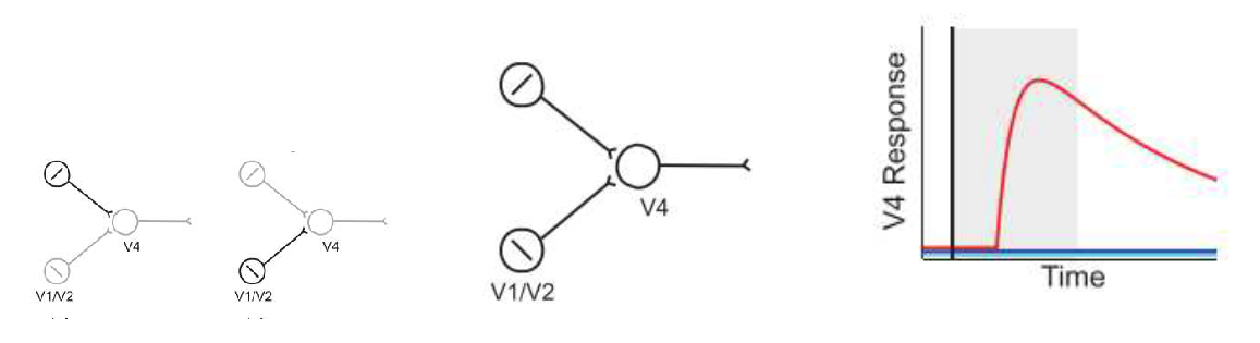
Yau et al. [35] argue that simultaneous multi-orientation inputs trigger recurrent neural networks that synthesize curvature. Without the recurrent network in place, the original line segments themselves do not excite a non-linear threshold model. Line segments at orientations 45 , 90 and 135 , were used and combined with B-spline approximations to form new curved segments.
Figure 11.
[33](p. 2) (a) Orientation inputs that fail to initiate recurrent network process for curvature synthesis (b) Orientation input, administered simultaneously, initiate recurrent network processes and generate a tuning curve for orientation components as seen in (c).
Figure 11.
[33](p. 2) (a) Orientation inputs that fail to initiate recurrent network process for curvature synthesis (b) Orientation input, administered simultaneously, initiate recurrent network processes and generate a tuning curve for orientation components as seen in (c).
El-Shamayleh and Pasupathy [29] show that the V4 neurons are scale-invariant by using differing scales of stimuli that have the same normalized curvature. Normalized curvature is described as the rate of change in tangent angle per unit of angular length. Absolute curvature is described as the rate of change in tangent angle with respect to contour length. When the shape scales up or down in relationship with object size, the normalized curvature remains the same while the absolute curvature changes. Most neurons maintained their selectivity for shape across size changes using normalized curvature as an explanation. A small proportion showed a shift in selectivity for shape when the object size changed.
Figure 12.
[29] (p. 2) (a) Absolute curvature (b) Normalized curvature.
Figure 12.
[29] (p. 2) (a) Absolute curvature (b) Normalized curvature.
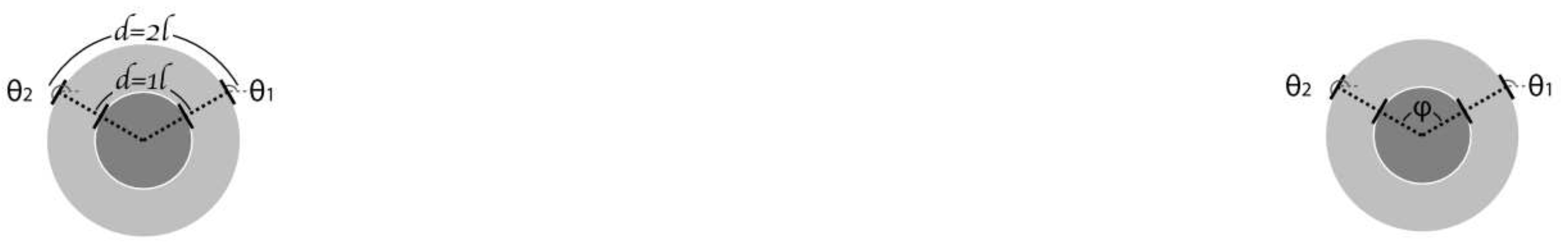
In earlier papers, Pasupathy and Connor [26,28] show the selectivity of V4 neurons for certain local contour curvature. El-Shamayleh and Pasupathy [29] extended the experiments by presenting the stimuli at different scales within its receptive field. Scale differentiates the normalized and absolute curvature definitions and the responses from their experiment show that V4 encodes objects in a size invariant manner and the normalized curvature definition better explains the responses observed in monkeys when comparing against the model that encodes normalized curvature.
An important feature of stimuli construction is the identification and boundary estimation of the receptive field. In Gattass et al. [30], the diameter of the receptive field in the V4 region is defined as
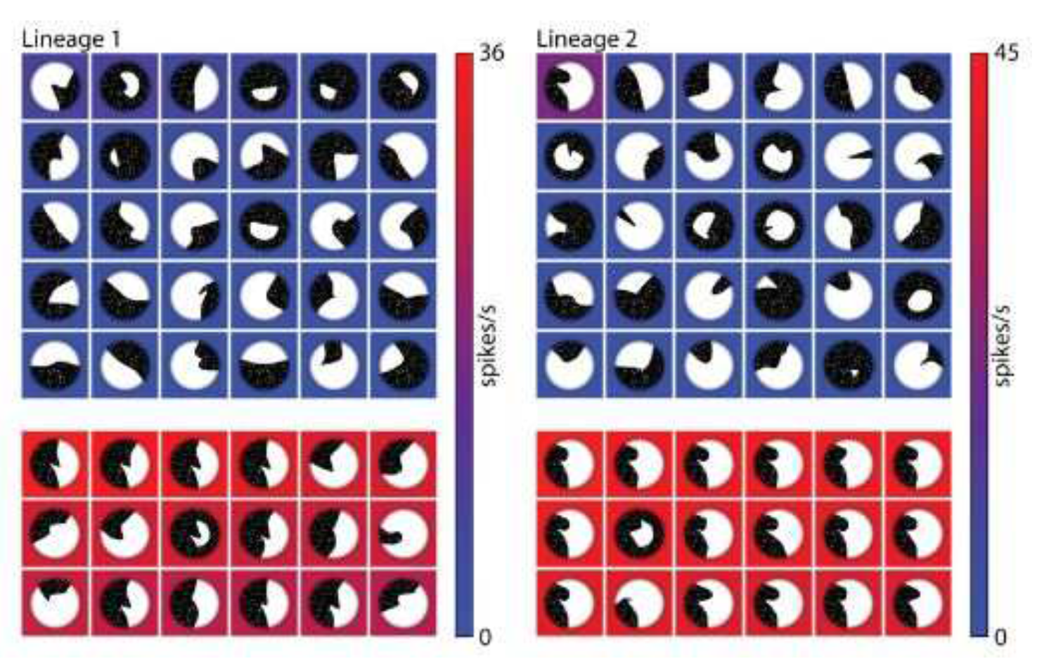
Carlson et al. [38] provide a synthetic evolutionary model that emulates sparse coding. The model adds control points during each generation, building new stimuli from Bezier splines, and generates strong population neural responses in V4 as it progresses. The results from the simulations are compared to the neural recordings from 165 V4 cells in monkeys. Higher responses are recorded in V4 towards contours containing acute convex or acute concave curvature. This preference for acuteness becomes defined as the sparseness constraints increase. The stimuli set is shown below.
Figure 13.
[38] (a) Set of stimulus constructed using incrementally added bezier splines. The left shows the neural spike responses for first generation stimuli. The right shows the neural spike responses from seventh generation stimuli.
Figure 13.
[38] (a) Set of stimulus constructed using incrementally added bezier splines. The left shows the neural spike responses for first generation stimuli. The right shows the neural spike responses from seventh generation stimuli.
Summarazing, the neural spikes, if representing linearly independent traits, can be combined together through a Gaussian product. The response can be made to fit an artificial neural network. However, state of the art synthetic neural networks are often too complex to fit weights to. We often study the responses from these systems rather than designing them from scratch.
Psychophysics
Contour completion using the association field
Von der Heydt and Peterhans [24] through their study of illusionary contours have shown that the contour is a combination of two operations. The first operation is the detection of borders by using contrast as the discriminatory feature and the second operation is aggregating occlusion features in a linear fashion.
The local range association field theory was proposed by Field et. al [39]. Field et. al exploit the redundancy in outputs from orientation selective Gabor filters to build a contour path even if the elements are not aligned in a straight line. Their perception of continuity was tested by altering five parameters: (1) relative orientation of path elements (2) elements orthogonal to path (3) selectivity along the path (4) inter element distance and (5) relative phase of the path elements. As long as the elements were less than in orientation, were separated no more than seven times the length of the element, end-to-end instead of side-to-side, the results in stringing elements to form a contour were strong. The association was orientation selective but not phase selective.
Figure 14.
[39] Association Field (a) Placement of path elements shows how the stimuli were created. D is the length of the segment. is the difference in the angle of orientation of successive path elements. is the angle of orientation of the sinusoid with respect to the path.(b) Vertically oriented filter applied to elements. Post filter application, specific paths are seen. (c) Stimulus presented in the experiment. (d) Contour detected within the stimulus.
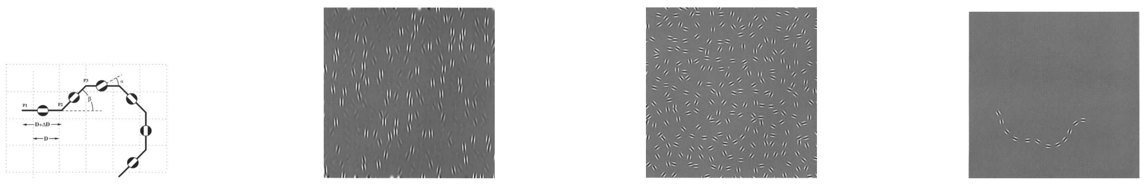
If neighbouring neurons in the cortex have receptive fields with collinear axes of preferred orientation, then these lateral interactions aid contour detection and completion. Removing or re-orienting a single Gabor patch in the path led to poorer performance, validating the above assumption [39,40]. In Pettet et al. [40], several Gabor patches were scattered in the experiment. The authors performed several simulations. The strength of the interaction was measured as a product of three standard Gaussian functions : (1) distance (2) total curvature and (3) change in curvature of a spline fit through the two receptive field. The total curvature was determined as a function of all three. Given a Gabor patch that is optimally tuned for orientation,position and scale, there is one neighbour that is optimally selected for processing that orientation,position and scale in a way to extend the contour towards completion.
Contour curvature closing by separable coding of tapering and axis curvature
It is shown through psychophysical study on curvature and tapering that distributed bell shaped tuning is a feature for the shape selectivity in the IT [41], similar to orientation frequency tuning in the early visual cortex. The joint tuning is separable and the product of the tuning in each direction can accurately predict shape characteristics.
This study builds a definition of a rectangle and a triangle on shape features such as axis curvature (bend), positive and negative curvature of the sides, taper and aspect ratio. Human psychophysical studies have shown that the properties of curvature, tapering and aspect ratio are independently coded [42,43]. The neural response in the shape space was studied using multi dimensional scaling (MDS). Each shape shown in Figure 15 was a point in the space. If the neurons select for the shape dimension orthogonally, the lower dimensional space also had solutions in which the orthogonal dimension would correspond to the manipulated shape dimension. Curvature is separably coded and the most important characteristic. A similar 3D computational model constructed by fitting a Gaussian function over the most excitatory presentation of the shape (3D) was built by Logothetis et al. [44].
Psychological contour curvature
Shape has also been perceptually studied in psychology. Attneave and Arnoult [23] suggest that in order to define a contour in terms of the distance between two segments and the slope in between them, a scale and orientation free definition could be given by the change in direction, the change in log of the length and the ratio of the distance between the apex of the angle and the shorter segment at which the arc approximates the curve.
Long range connections
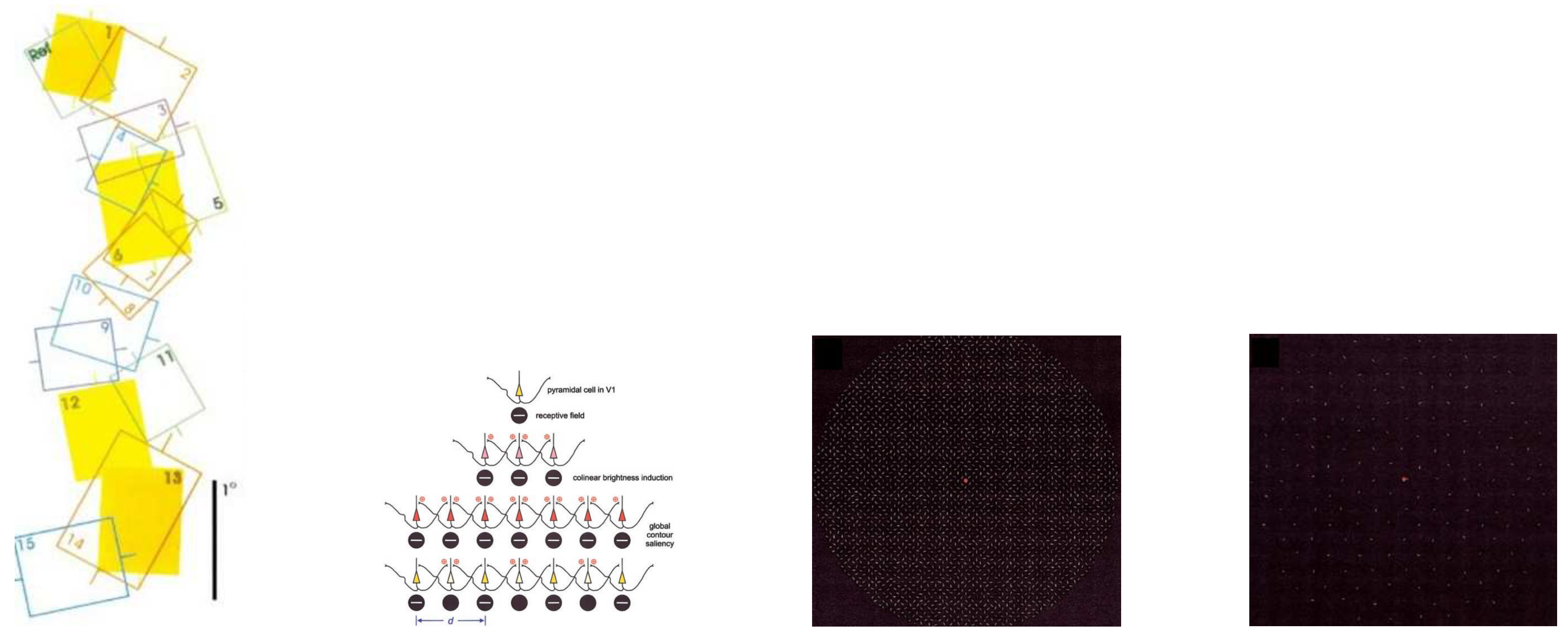
Das and Gilbert [21] showed a relationship between receptive field and orientation by measuring changes in receptive field as a function of changes in orientation preference. Irrespective of where the recording was done, a change in orientation preference was associated with a translation of two receptive fields such that there was no overlap between the original receptive field and the location two receptive fields length away. They also showed that the receptive fields of similar orientations cluster together and receptive fields of orthogonal orientations do not overlap. Occasionally a orthogonal receptive field cluster might lie adjacent to its orthogonal counterpart, allowing for concurrent processing of contours in areas as early as V1.
Li and Gilbert [22] show that if the distance between two collinear segments is very large, outside of the reach of a horizontal connection link, the segments will not form a contour. Likewise, if the density of noisy randomly oriented elements is too high, no contour will pop out. Both the spacing between segments and the density of segments play a role in the critical construction of the contour. In Figure 17c,d, one figure shows a dense region of segments whereas the second figure has very sparse segments. The second figure does not allow the formation of contour percepts.
Conclusion
While a lot of work has been done trying to understand the stimuli or shape characteristics to which each of the regions (V1,V2 and V4) show selectivity for, the topographical build-up in a hierarchical way is missing.
While single units in area V4 demonstrate tuning for orientation and angle when presented in isolation in the cell’s receptive field, complex shapes show preference for curvature at boundary locations within the larger shape. It is unclear if the brain builds a topographical build up by using component features in lower regions of the brain in a clear combinatorial way. As receptive fields are biological units, relying heavily on the additive receptive field orientations within the cortical column, a straight forward definition of the contour independent of eccentricity remains elusive.
Psychophysical experiments show how the curvature could be modelled in the cortex. Understanding the various neuroscience models in conjunction with the psychophysical experiments conducted confirm that the cortex is often responsible for most of the curvature formation in human vision. However, systems neuroscience studies operating directly on the cortex in macaques are both expensive and invasive. As curvature formation is dependent on the underlying anatomical physiology, a lot of open areas remain unexplored in the study of curvature, in terms of mapping the spatial presentation of stimuli on the retina exploiting neurophysiology to the biological formation of shape in easily representable mathematical form.
References
- Hess R and Field D (1999) Integration of contours: New insights. Trends in Cognitive Sciences, 3(12), 480 – 486.
- Wertheimer M (1923) Untersuchungen zur Lehre von der Gestalt. II. Psychologische Forschung. 1923. Vol. 4(1):301-350. [CrossRef]
- Zucker SW and Dobbins A and Iverson L (1989) Two stages of curve detection suggest two styles of visual computation. Neural Computation, 1(1), 68–81.
- Feldman J (2001) Bayesian contour integration. Perception & Psychophysics, 63(7), 1171 – 1182.
- Jain RC and Kasturi R and Schunck BG (1995) Machine vision. McGraw-Hill. ISBN: 978-0-07-032018-5. 9: ISBN.
- Elder JH (2018) Shape from Contour: Computation and Representation. Annu Rev Vis Sci. 2018 Sep 15;4:423-450. [CrossRef]
- Koenderink JJ (1984) What Does the Occluding Contour Tell Us about Solid Shape? Perception, 13, 321 - 330.
- Hubel DH and Wiesel TN (1959) Receptive fields of single neurones in the cat’s striate cortex. J Physiol. 1959 Oct;148(3):574-91.
- Hubel DH and Wiesel TN (1962) Receptive fields, binocular interaction and functional architecture in the cat’s visual cortex. Journal of Physiology (London), 160(1), 106–154.
- Kuffler SW (1953) Discharge patterns and functional organization of mammalian retina. J Neurophysiol. 1953 Jan;16(1):37-68. [CrossRef]
- Palmer SE (1999) Vision science: Photons to phenomenology. The MIT Press.
- Hubel DH and Wiesel TN (1965) Receptive fields and functional architecture in two nonstriate visual area (18 and 19) of the cat. J Neurophysiol. 1965 Mar;28:229-89. [CrossRef]
- Hubel DH (1968) Receptive fields and functional architecture of monkey striate cortex. J Physiol. 1968 Mar;195(1):215-43. [CrossRef]
- Heitger F, Rosenthaler L, von der Heydt R, Peterhans E and Kübler O (1992) Simulation of neural contour mechanisms: from simple to end-stopped cells. Vision Res. 1992 May;32(5):963-81. [CrossRef]
- Dobbins A and Zucker SW and Cynader MS (1987) Endstopped neurons in the visual cortex as a substrate for calculating curvature. Nature. 1987 Oct 1-7;329(6138):438-41. [CrossRef]
- Versave M and Orban GA and Lagae L (1990) Responses of visual cortical neurons to curved stimuli and chevrons. Vision Res. 1990;30(2):235-48. [CrossRef]
- Turner MR (1986) Texture discrimination by Gabor functions. Biol Cybern. 1986;55(2-3):71-82. [CrossRef]
- Orban GA (2008) Higher order visual processing in macaque extrastriate cortex. Physiol Rev. 2008 Jan;88(1):59-89. [CrossRef]
- Hegde J and Van Essen DC (2000) Selectivity for complex shapes in primate visual area V2. J Neurosci. 2000 Mar 1;20(5):RC61. [CrossRef]
- Hegde J and Van Essen DC (2007) A comparative study of shape representation in macaque visual areas V2 and V4. Cerebral Cortex, 17(5), 1100–1116.
- Das A and Gilbert C (1997) Distortions of visuotopic map match orientation singularities in primary visual cortex. Nature 387, 594–598 (1997). [CrossRef]
- Li W and Gilbert CD (2002) Global contour saliency and local colinear interactions. J Neurophysiol. 2002 Nov;88(5):2846-56. [CrossRef]
- Attneave F and Arnoult MD (1956) The quantitative study of shape and pattern perception. Psychological Bulletin, 53(6), 452–471. [CrossRef]
- Peterhans E and von der Heydt R (1989) Mechanisms of contour perception in monkey visual cortex. II. Contours bridging gaps. J Neurosci. 1989 May;9(5):1749-63. [CrossRef]
- Gattass R, Gross CG and Sandell JH (1981) Visual topography of V2 in the macaque. J Comp Neurol. 1981 Oct 1;201(4):519-39. [CrossRef]
- Pasupathy A and Connor CE (1999) Responses to contour features in macaque area V4. Journal of Neurophysiology, 82(5), 2490–2502.
- Pasupathy A and Connor CE (2002) Population coding of shape in area V4. Nat Neurosci. 2002 Dec;5(12):1332-8. [CrossRef]
- Pasupathy A and Connor CE (2001) Shape representation in area V4: position-specific tuning for boundary conformation. J Neurophysiol. 2001 Nov;86(5):2505-19. [CrossRef]
- El-Shamayleh Y and Pasupathy A (2016) Contour Curvature As an Invariant Code for Objects in Visual Area V4. J Neurosci. 2016 ;36(20):5532-43. 18 May. [CrossRef]
- Gattass R, Sousa AP, Gross CG (1988) Visuotopic organization and extent of V3 and V4 of the macaque. J Neurosci. 1988 Jun;8(6):1831-45. [CrossRef]
- Gallant JL, Connor CE, Rakshit S, Lewis JW and Van Essen DC (1996) Neural responses to polar, hyperbolic, and Cartesian gratings in area V4 of the macaque monkey. J Neurophysiol. 1996 Oct;76(4):2718-39. [CrossRef]
- Das A and Gilbert CD (1999) Topography of contextual modulations mediated by short-range interactions in primary visual cortex. Nature. 1999 Jun 17;399(6737):655-61. [CrossRef]
- Das A and Gilbert CD (1997) Distortions of visuotopic map match orientation singularities in primary visual cortex. Nature. 1997 Jun 5;387(6633):594-8. [CrossRef]
- Gheorghiu E and Kingdom FA (2009) Gheorghiu E, Kingdom FA. Multiplication in curvature processing. J Vis. 2009 Feb 27;9(2):23.1-17. [CrossRef]
- Yau JM, Pasupathy A, Brincat SL and Connor CE (2013) Curvature processing dynamics in macaque area V4. Cereb Cortex. 2013 Jan;23(1):198-209. [CrossRef]
- Wolfe JM, Yee A and Friedman-Hill SR (1992) Wolfe JM, Yee A, Friedman-Hill SR. Curvature is a basic feature for visual search tasks. Perception. 1992;21(4):465-80. [CrossRef]
- Chen S and Levi DM (1996) Chen S, Levi DM. Angle judgement: is the whole the sum of its parts? Vision Res. 1996 Jun;36(12):1721-35. [CrossRef]
- Carlson ET, Rasquinha RJ, Zhang K and Connor CE (2011) A sparse object coding scheme in area V4. Curr Biol. 2011 Feb 22;21(4):288-93. [CrossRef]
- Field DJ, Hayes A and Hess RF (1993) Field DJ, Hayes A, Hess RF. Contour integration by the human visual system: evidence for a local "association field". Vision Res. 1993 Jan;33(2):173-93. [CrossRef]
- Pettet MW, McKee SP and Grzywacz NM (1998) Constraints on long range interactions mediating contour detection. Vision Res. 1998 Mar;38(6):865-79. [CrossRef]
- Kayaert G, Biederman I, de Beeck HPO and Vogels R (2005) Tuning for shape dimensions in macaque inferior temporal cortex. European Journal of Neuroscience, 22(1), 212–224.
- Stankiewicz BJ (2002) Stankiewicz BJ. Empirical evidence for independent dimensions in the visual representation of three-dimensional shape. J Exp Psychol Hum Percept Perform. 2002 Aug;28(4):913-32.
- Op de Beeck H, Wagemans J and Vogels R (2003) The effect of category learning on the representation of shape: dimensions can be biased but not differentiated. J Exp Psychol Gen. 2003 Dec;132(4):491-511. [CrossRef]
- Logothetis NK, Pauls J and Poggio T (1995) Logothetis NK, Pauls J, Poggio T. Shape representation in the inferior temporal cortex of monkeys. Curr Biol. 1995 ;5(5):552-63. 1 May. [CrossRef]
Figure 1.
The reciprocal of , otherwise known as the radius of the osculating circle, represents the curvature.
Figure 1.
The reciprocal of , otherwise known as the radius of the osculating circle, represents the curvature.
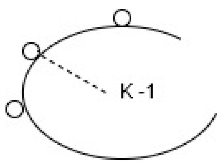
Figure 2.
[6] (p. 424) Parts of the polar bear are visible to the eye and parts of the polar bear are invisible to the eye. The rim demarcates the boundary of what is visible and what is invisible. From the vantage point of the eye, the rim projects on a plane that is normal to the visual direction. This projection is a 2D region bound by a 1D curve, called the contour.
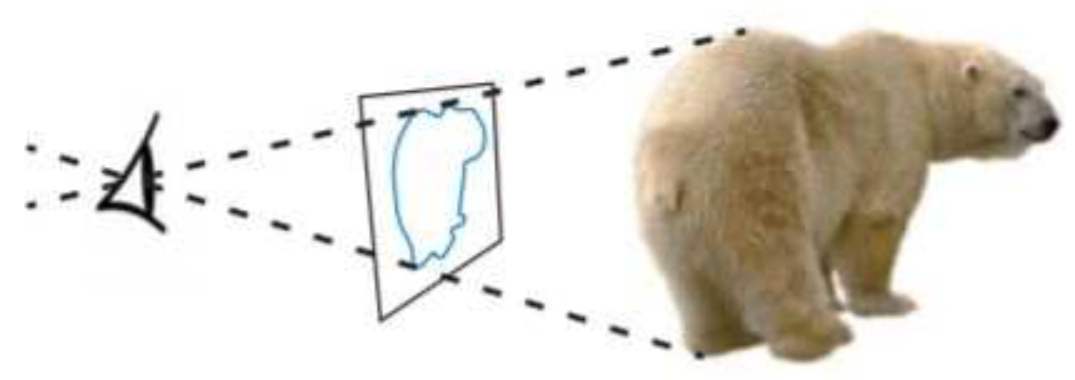
Figure 3.
[11] (p. 152) (a,b) Lateral Geniculate Nuclues (LGN) cells with on and off excitation regions (c) Edge Detectors (d) Line Detectors (e) (p. 170) A vertical Gabor function that acts like a vertical edge detector.
Figure 3.
[11] (p. 152) (a,b) Lateral Geniculate Nuclues (LGN) cells with on and off excitation regions (c) Edge Detectors (d) Line Detectors (e) (p. 170) A vertical Gabor function that acts like a vertical edge detector.

Figure 4.
(a) Special zero-mean functions that are similar to Gabor functions in spatially filtering properties but have zero integral. The special functions are shown in solid lines while the Gabors are shown in dashed lines. (b) A : Intensity profile of an image showing bright and dark regions B,C: image convolved with odd and even operators D: output of the energy terms operator. It shows spikes where the contrast is high. (c) End stopped cells help to shape the definition of a contour or angle. (a),(b) [14] (p. 965,968) , (c) from [18] (p. 80).
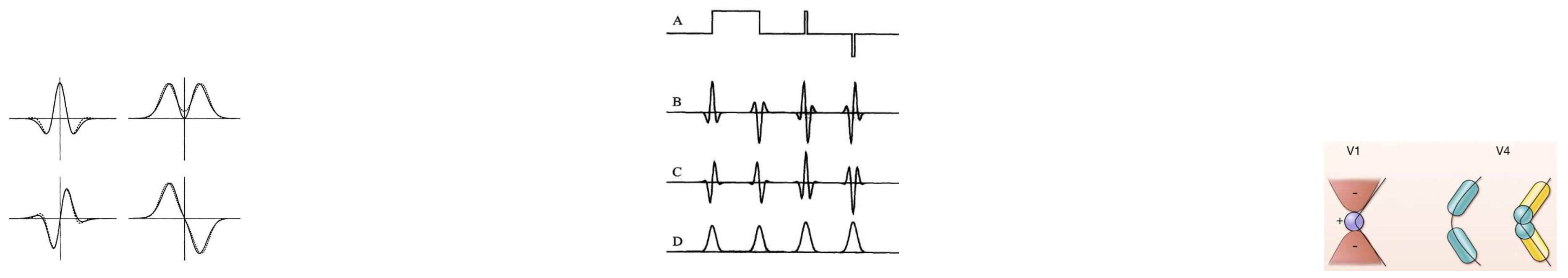
Figure 5.
[14] (p. 976) (a) Local maxima from the energy term shows contrast boundary (b) Key points (c) Single stopped cells evaluated at the key points.
Figure 5.
[14] (p. 976) (a) Local maxima from the energy term shows contrast boundary (b) Key points (c) Single stopped cells evaluated at the key points.
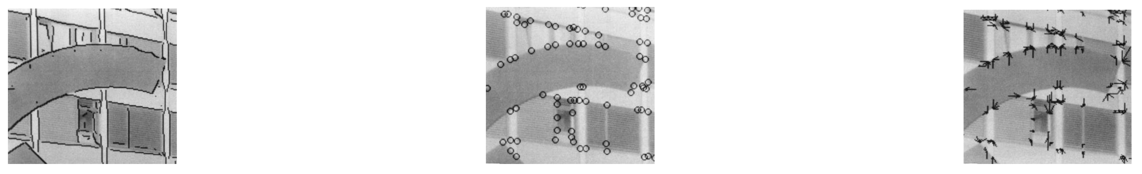
Figure 6.
[19] (p. 3) (a) V2 cells that show a preference for acute and right angles oriented in particular way. Orientations have been normalized to point vertically in the figure for the most preferred orientation. (b) V2 cells that show preference for arc and circles and complex contours such as hyperbolic gratings.
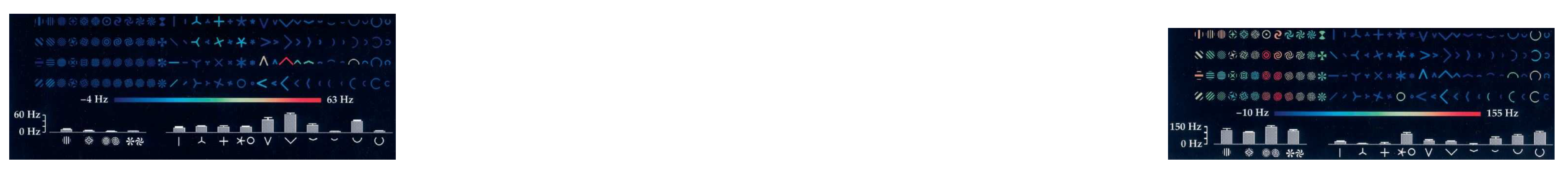
Figure 7.
[33] (p. 596) Receptive fields with similar orientation clustered together.
Figure 7.
[33] (p. 596) Receptive fields with similar orientation clustered together.
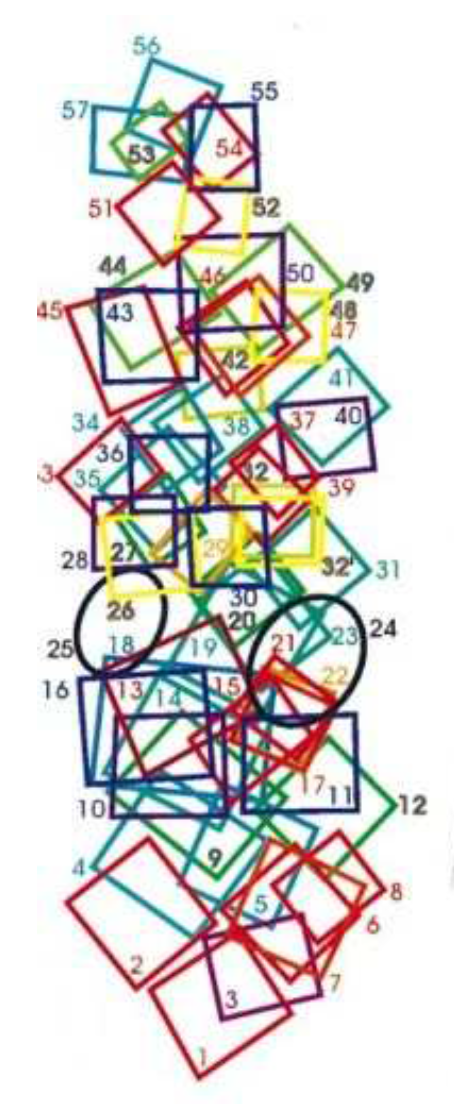
Figure 8.
[26] (p. 3) Stimuli presented to test for contour features: (a) sharp convex (b) sharp outline (c) sharp concave (d) smooth convex (e) Stimulus set, a function of (convexity, curvature, acuteness); (f) Stimulus exhibiting the strongest response.
Figure 8.
[26] (p. 3) Stimuli presented to test for contour features: (a) sharp convex (b) sharp outline (c) sharp concave (d) smooth convex (e) Stimulus set, a function of (convexity, curvature, acuteness); (f) Stimulus exhibiting the strongest response.
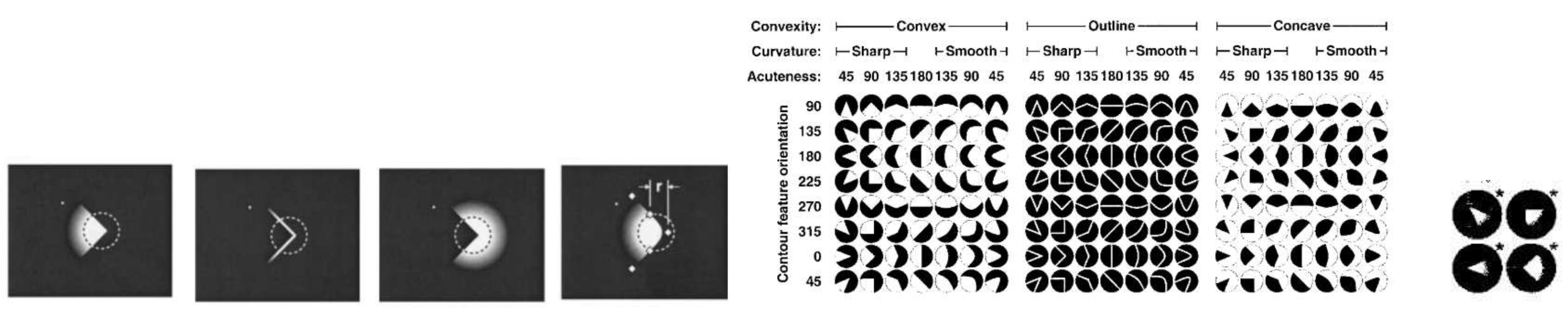
Figure 9.
[27](p. 3) (a) Population neural response to stimuli presented on the orientation-curvature domain. Red marks highest firing rates (b) Decoded stimulus from the neural response.
Figure 9.
[27](p. 3) (a) Population neural response to stimuli presented on the orientation-curvature domain. Red marks highest firing rates (b) Decoded stimulus from the neural response.
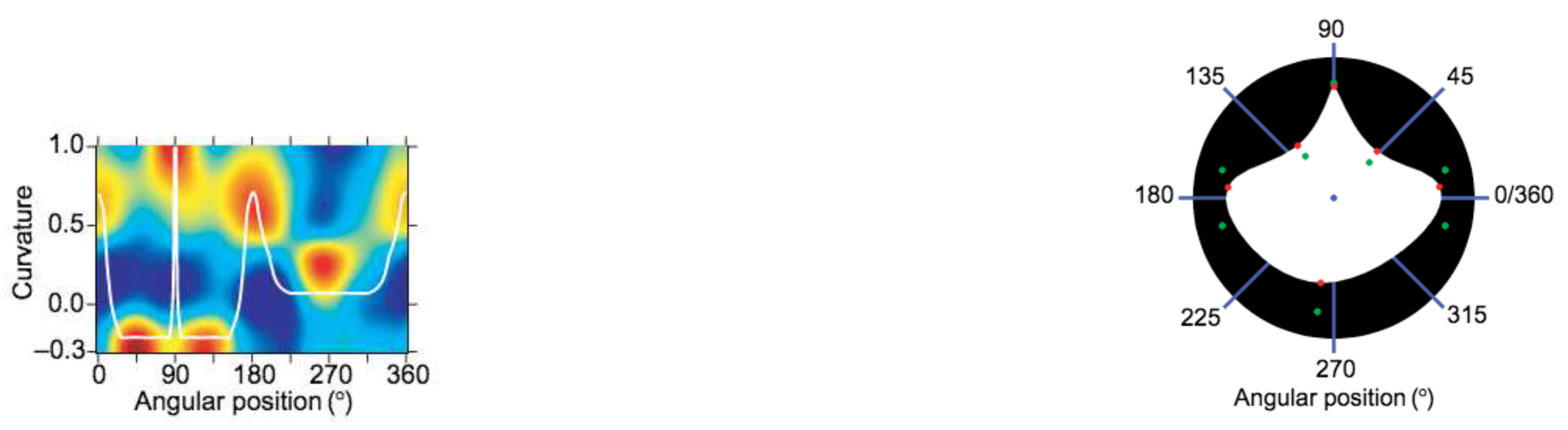
Figure 10.
[28](p. 3) Stimuli presented to test for boundary features: (a) Stimulus set, a function of (curvature, orientation, angular position and radial position). Each group is a particular configuration of convex projections and the number of such projections. The angular separations between convex projections were multiples of 45 degrees. For example, 4 convex projections separated by 90 degrees is represented by the right most block.
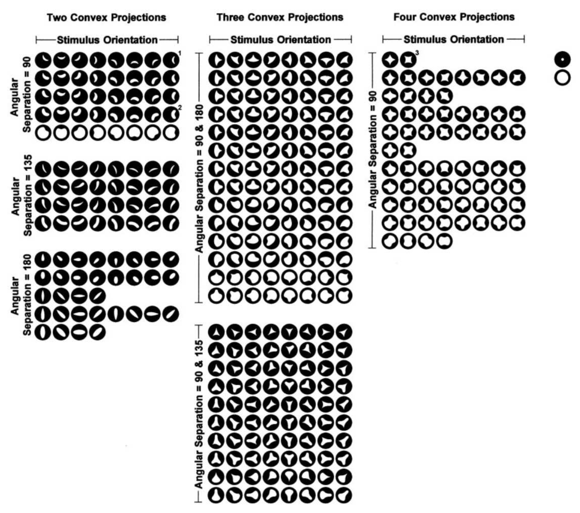
Figure 15.
(a) Spline fitting algorithm for determining curvature interaction (b).
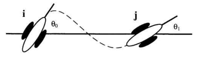
Figure 16.
(a) Rectangle defined by bend or axis curvature, positive and negative curvature of the sides using the ’curve’ function and the taper function (b) Two dimensions vary: negative curvature and taper (c) Two dimensions vary: axis curvature and taper (d) axis curvature and aspect ratio of the triangle.
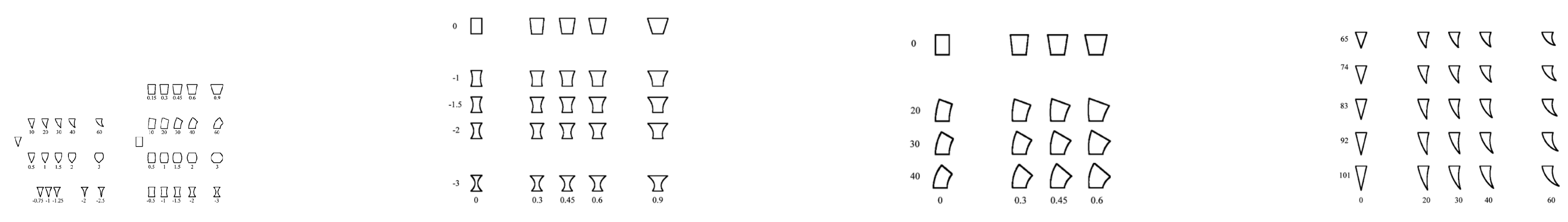
Figure 17.
(a) Receptive fields with the orthogonal receptive field showing no overlap with its 90 degree counterpart. This allows population neurons to fire only for 45 and 135 degree for example, with no recorded response for angles in between. (b) Rows 1-3 allow for reinforced collinear integration of contour path. Contour closure experiences a breakdown in row 4 when a large gap occurs during integration. (d,e) Contour closure and detection decreases with decreasing density of segments. An optimal density produces detectable contours. (c) shows better contour detection than (d). Figure (a,b) from [21] ; (c,d) from [22].
Disclaimer/Publisher’s Note: The statements, opinions and data contained in all publications are solely those of the individual author(s) and contributor(s) and not of MDPI and/or the editor(s). MDPI and/or the editor(s) disclaim responsibility for any injury to people or property resulting from any ideas, methods, instructions or products referred to in the content. |
© 2023 by the authors. Licensee MDPI, Basel, Switzerland. This article is an open access article distributed under the terms and conditions of the Creative Commons Attribution (CC BY) license (http://creativecommons.org/licenses/by/4.0/).
Copyright: This open access article is published under a Creative Commons CC BY 4.0 license, which permit the free download, distribution, and reuse, provided that the author and preprint are cited in any reuse.


