New Soliton Solutions of M-fractional Westervelt Model in Ultrasound Imaging via Two Analytical Techniques

1. Introduction

Soliton theory based on water waves, plasmas, optical fibers etc., was developed in 1960-1970. This is significant branch of applied mathematics as well as mathematical physics. It has significant uses in nonlinear optics, fluid mechanics, plasmas etc. This theory is widely applied in various natural sciences, including communication, biology, chemistry, mathematics and almost all branches of physics including fluid dynamics, condensed matter physics, plasma physics and in others.

Various naturally occurring phenomenon are shown as a nonlinear partial differential equations (NLPDEs). A variety of techniques are made to attain results for NLPDEs. For examples, modified direct algebraic technique [1], modified Khater scheme [2], generalized Kudryashov scheme [3], novel $(G^{\prime }/G)$-expansion method [4], extended mapping scheme [5].

There are two another straight forward, fruitful and reliable techniques; ${exp}_a$ function technique and modified simplest equation technique. There are various uses of these techniques. Instantly; optical wave solutions of perturbed Gerdjikov-Ivanov model by utilizing the ${exp}_a$ function scheme [6], some new optical solitons of Sasa-Satsuma higher order equation in [7], the dark soliton, bright soliton and combo optical solitons of three coupled Maccari’s model are attained [8], dark, bright and many other exact wave solutions of modified Camassa-Holm model are obtained in [9]. Similarly, some solitary wave solutions of BBM and Chan-Hilliard equations by utilizing modified simplest equation method [10], exact wave solutions of Boussinesq and coupled Boussinesq equations are obtained by using this method [11].

Our study model is the Westervelt equation along truncated M-fractional derivative. Different kinds of analytical wave solitons of concerned model are achieved by distinct techniques. For example, exact solitary wave solitons have been achieved by utilizing modified Kudryashov and generalized Kudryashov schemes [12], the periodic, exponential, hyperbolic and plane wave functions solutions are gained with the use of modified exponential rational function and modified $(G^{\prime }/G^2)$-Expansion techniques [13].

Basic aim of our research is to attain the new soliton solutions to M-fractional Westervelt model via ${exp}_a$ function and modified simplest equation techniques.

Our paper contains 5 sections; 2nd-section is about the aforementioned model and it’s mathematical analysis, 3rd-section is concerned about ${exp}_a$ function technique and it’s application to get the soliton solutions, 4th-section explain the modified simplest equation technique and apply it to get soliton solutions, 5th-section is about the explanation of some gained results by 2-dimensional, 3-dimensional and contour plots and 6th-section is the conclusion.

2. Governing model and It’s mathematical analysis

Let’s assume the space-time fractional Westervelt model given as [13]:

$$2\tau (u{D}_{M,t}^{\alpha ,{\rm Y}}u+{\left(D_{M,t}^{\alpha ,{\rm Y}}u\right)}^2)+{\rho }^2{D}_{M,2x}^{2\alpha ,{\rm Y}}u+\theta D_{M,t}^{\alpha ,{\rm Y}}\left(D_{M,2x}^{2\alpha ,{\rm Y}}u\right)-D_{M,t}^{\alpha ,{\rm Y}}u=0.$$

(1)

here

$$D_{M,t}^{\alpha ,{\rm Y}}u\left(t\right)=\underset{\tau \to 0}{lim}\frac{u\left(t{E}_{{\rm Y}}\left(\tau t^{1-\alpha }\right)\right)-u\left(t\right)}{\tau },\alpha \in (0,1],{\rm Y}>0,$$

(2)

where $E_{{\rm Y}}(.)$ denotes truncated Mittag-Leffler (TML) function shown in [14,15]. here u=u(x,t) indicates the real wave function. Parameters $\theta$ denotes the diffusivity of sound and $\rho$ represents the speed of sound. The non-linearity parameter $\tau =\frac{1+\frac{B}{2A}}{f}$ where f is the bulk modulus which is taken as $f=\eta {\rho }^2$ and $\eta$ is working as the mass density.

Applying the given wave transformations:

$$u(x,t)=U\left(\xi \right),\xi =\frac{\Gamma ({\rm Y}+1)}{\alpha }(\lambda x^{\alpha }+\delta t^{\alpha })$$

(3)

here parameters $\lambda$ and $\delta$ are the spatio and temporal coefficients. By applying Eq.(3) into Eq.(1), we get a NLODE shown as:

$$\delta \theta {\lambda }^2{U}^{{}^{‴}}+{\lambda }^2{\rho }^2{U}^{″}+{\delta }^2\left(2\tau U{U}^{″}-U^{″}+{\left(U^{\prime }\right)}^2\right)=0$$

(4)

where U denotes the polynomial and prime ${}^{\prime }$ represents the $\frac{d}{d\xi }$. By applying Homogenous Balance method, we get m=1. We will find new soliton solutions of Eq.(4) by applying two different techniques in the following.

3. The ${exp}_{\mathbf{a}}$ function technique

Here we mention the basic steps of this technique.

Assuming a NLPDE;

$$F(f,f^2{f}_y,f_t,f_{xy},f_{tt},f_{yt},...)=0.$$

(5)

Eq .(5) changed into NLODE:

$$Y(F,F^{{}^{\prime }},F^{{}^{″}},...,)=0.$$

(6)

By using the given wave transformations:

$$f(x,y,t)=F\left(\xi \right),\xi =\delta x+\mu y+\lambda t.$$

(7)

Assuming the results of Eq. (6) are shown in [16,17,18,19]:

$$F\left(\xi \right)=\frac{{\alpha }_0+{\alpha }_1{d}^{\xi }+...+{\alpha }_m{d}^{m\xi }}{{\beta }_0+{\beta }_1{d}^{\xi }+...+{\beta }_m{d}^{m\xi }},d\ne 0,1.$$

(8)

here ${\alpha }_j$ and ${\beta }_j(0\le j\le m)$ are the undetermined. Natural number m is found with the use of homogenous balance technique into Eq. (8). Inserting Eq.(8) into Eq.(6), results

$$\wp \left(d^{\xi }\right)={\ell }_0+{\ell }_1{d}^{\xi }+...+{\ell }_t{d}^{t\xi }=0,.$$

(9)

Inserting ${\ell }_j(0\le j\le t)$ into Eq. (9) taking zeo, a system of equations is attained:

$${\ell }_j=0,herej=0,...,t.$$

(10)

Applying obtain solutions, one can get exact solitons for Eq. (5).

3.1. New wave solutions by the ${exp}_a$ function technique

Eq.(8) reduces into below form for m=1:

$$U\left(\xi \right)=\frac{{\alpha }_0+{\alpha }_1{d}^{\xi }}{{\beta }_0+{\beta }_1{d}^{\xi }}$$

(11)

Substituting Eq.(11) into Eq.(4), a set of equations is gained. Evaluating these, we get distinct sets:

Set 1:

$$\left\{{\alpha }_0=\frac{{\beta }_0\left({\delta }^2-\delta \theta {\lambda }^{2}log\left(d\right)-{\lambda }^2{\rho }^2\right)}{{\delta }^2},{\alpha }_1=\frac{{\beta }_1\left({\delta }^2+\delta \theta {\lambda }^{2}log\left(d\right)-{\lambda }^2{\rho }^2\right)}{{\delta }^2},\tau =\frac{1}{2}\right\}$$

(12)

$$u(x,t)=\frac{{\beta }_1{d}^{\xi }\left({\delta }^2+\delta \theta {\lambda }^{2}log\left(d\right)-{\lambda }^2{\rho }^2\right)+{\beta }_0\left({\delta }^2-\delta \theta {\lambda }^{2}log\left(d\right)-{\lambda }^2{\rho }^2\right)}{{\delta }^2\left({\beta }_0+{\beta }_1{d}^{\xi }\right)}$$

(13)

Set 2:

$$\left\{{\alpha }_1=-\frac{{\beta }_1\left({\delta }^2+\delta \theta {\lambda }^{2}log\left(d\right)-{\lambda }^2{\rho }^2\right)}{{\delta }^2},{\beta }_0=0,\tau =-\frac{1}{2}\right\}$$

(14)

$$u(x,t)=\frac{{\alpha }_0{\delta }^2-{\beta }_1{d}^{\xi }\left({\delta }^2+\delta \theta {\lambda }^{2}log\left(d\right)-{\lambda }^2{\rho }^2\right)}{{\beta }_1{\delta }^2{d}^{\xi }}$$

(15)

Set 3:

$$\left\{{\alpha }_0=-\frac{{\beta }_0\left({\delta }^2-\delta \theta {\lambda }^{2}log\left(d\right)-{\lambda }^2{\rho }^2\right)}{{\delta }^2},{\beta }_1=0,\tau =-\frac{1}{2}\right\}$$

(16)

$$u(x,t)=\frac{{\alpha }_1{\delta }^2{d}^{\xi }+{\beta }_0\left(-{\delta }^2+\delta \theta {\lambda }^{2}log\left(d\right)+{\lambda }^2{\rho }^2\right)}{{\beta }_0{\delta }^2}$$

(17)

4. Modified simplest equation technique

Here we point out the some main steps of this technique.

Step 1:

Supposing a NLPDE:

$$G(f,f^2{f}_y,f_t,f_{xy},f_{tt},f_{yt},...)=0,$$

(18)

where $f=f(x,y,t)$ represents a wave profile.

Consider the wave transformation:

$$f(x,y,t)=F\left(\xi \right),\xi =x-\mu y+\lambda t.$$

(19)

Substituting Eq. (19) into Eq. (18), we gain the NLODE:

$$Z(F,F^2{F}^{{}^{\prime }},F^{{}^{″}},...)=0.$$

(20)

Step 2: Let Eq.(20) has the solution form:

$$F\left(\xi \right)=\sum _{j=1}^m{b}_j{\psi }^j\left(\xi \right)$$

(21)

here $b_j(j=1,2,...,m)$ are unknowns and $b_m\ne 0$.

A new function $\psi \left(\xi \right)$ fulfil below ODE:

$${\psi }^{\prime }\left(\xi \right)={\psi }^2\left(\xi \right)+\eta$$

(22)

here $\eta$ is a .

Eq.(22) have solutions for different cases of $\eta$:

Case 1: if $\eta <0$,

$$\psi \left(\xi \right)=-\sqrt{-\eta }tanh\left(\sqrt{-\eta }\xi \right)$$

(23)

$$\psi \left(\xi \right)=-\sqrt{-\eta }coth\left(\sqrt{-\eta }\xi \right)$$

(24)

$$\psi \left(\xi \right)=\sqrt{-\eta }\left(-tanh\left(2\sqrt{-\eta }\xi \right)\pm isech\left(2\sqrt{-\eta }\xi \right)\right),$$

(25)

$$\psi \left(\xi \right)=\sqrt{-\eta }\left(-coth\left(2\sqrt{-\eta }\xi \right)\pm csch\left(2\sqrt{-\eta }\xi \right)\right),$$

(26)

$$\psi \left(\xi \right)=-\frac{\sqrt{-\eta }}{2}\left(tanh\left(\frac{\sqrt{-\eta }}{2}\xi \right)+coth\left(\frac{\sqrt{-\eta }}{2}\xi \right)\right).$$

(27)

Case 2: if $\eta >0$,

$$\psi \left(\xi \right)=\sqrt{\eta }tan\left(\sqrt{\eta }\xi \right)$$

(28)

$$\psi \left(\xi \right)=-\sqrt{\eta }cot\left(\sqrt{\eta }\xi \right)$$

(29)

$$\psi \left(\xi \right)=\sqrt{\eta }\left(tan\left(2\sqrt{\eta }\xi \right)\pm sec\left(2\sqrt{\eta }\xi \right)\right),$$

(30)

$$\psi \left(\xi \right)=\sqrt{\eta }\left(-cot\left(2\sqrt{\eta }\xi \right)\pm csc\left(2\sqrt{\eta }\xi \right)\right),$$

(31)

$$\psi \left(\xi \right)=\frac{\sqrt{\eta }}{2}\left(tan\left(\frac{\sqrt{\eta }}{2}\xi \right)-cot\left(\frac{\sqrt{\eta }}{2}\xi \right)\right).$$

(32)

Case 3: if $\eta =0$,

$$\psi \left(\xi \right)=-\frac{1}{\xi }$$

(33)

Step 3: Applying Eq.(21) and Eq.(22) into Eq.(20) and sum up the co-efficients of every power of ${\psi }^j$. Substituting co-efficients of each power equal to zero, we obtain a set of equations involving $b_i$, $\lambda$, $\mu$. Evaluating the gained set of equations, we gain results.

Step 4: Inserting Eq.(21) of which $b_j$, $\lambda$, $\mu$ has been obtained into Eq.(20), we gain analytical wave solutions of Eq.(18).

4.1. New soliton solutions of Eq.(4) by MSET

Eq.(21) reduces for m=1:

$$U\left(\xi \right)=b_0+b_1\psi \left(\xi \right)$$

(34)

Using Eq.(34) into Eq.(4) with Eq.(20), we obtain solution.

Set:

$$\left\{b_0=\frac{{\delta }^2-{\lambda }^2{\rho }^2}{{\delta }^2},b_1=-\frac{2\theta {\lambda }^2}{\delta },\tau =\frac{1}{2}\right\}$$

(35)

Case 1: If $\eta <0$,

$$u(x,t)=\frac{{\delta }^2-{\lambda }^2{\rho }^2}{{\delta }^2}-\frac{2\theta {\lambda }^2}{\delta }(-\sqrt{-\eta }tanh\left(\sqrt{-\eta }\xi \right))$$

(36)

$$u(x,t)=\frac{{\delta }^2-{\lambda }^2{\rho }^2}{{\delta }^2}-\frac{2\theta {\lambda }^2}{\delta }(-\sqrt{-\eta }coth\left(\sqrt{-\eta }\xi \right))$$

(37)

$$u(x,t)=\frac{{\delta }^2-{\lambda }^2{\rho }^2}{{\delta }^2}-\frac{2\theta {\lambda }^2}{\delta }\left(\sqrt{-\eta }\left(-tanh\left(2\sqrt{-\eta }\xi \right)\pm isech\left(2\sqrt{-\eta }\xi \right)\right)\right)$$

(38)

$$u(x,t)=\frac{{\delta }^2-{\lambda }^2{\rho }^2}{{\delta }^2}-\frac{2\theta {\lambda }^2}{\delta }\left(\sqrt{-\eta }\left(-coth\left(2\sqrt{-\eta }\xi \right)\pm csch\left(2\sqrt{-\eta }\xi \right)\right)\right)$$

(39)

$$u(x,t)=\frac{{\delta }^2-{\lambda }^2{\rho }^2}{{\delta }^2}-\frac{2\theta {\lambda }^2}{\delta }(-\frac{\sqrt{-\eta }}{2}\left(tanh\left(\frac{\sqrt{-\eta }}{2}\xi \right)+coth\left(\frac{\sqrt{-\eta }}{2}\xi \right)\right))$$

(40)

Case 2:

$$u(x,t)=\frac{{\delta }^2-{\lambda }^2{\rho }^2}{{\delta }^2}-\frac{2\theta {\lambda }^2}{\delta }(\sqrt{\eta }tan\left(\sqrt{\eta }\xi \right))$$

(41)

$$u(x,t)=\frac{{\delta }^2-{\lambda }^2{\rho }^2}{{\delta }^2}-\frac{2\theta {\lambda }^2}{\delta }(-\sqrt{\eta }cot\left(\sqrt{\eta }\xi \right))$$

(42)

$$u(x,t)=\frac{{\delta }^2-{\lambda }^2{\rho }^2}{{\delta }^2}-\frac{2\theta {\lambda }^2}{\delta }\left(\sqrt{\eta }\left(tan\left(2\sqrt{\eta }\xi \right)\pm sec\left(2\sqrt{\eta }\xi \right)\right)\right)$$

(43)

$$u(x,t)=\frac{{\delta }^2-{\lambda }^2{\rho }^2}{{\delta }^2}-\frac{2\theta {\lambda }^2}{\delta }\left(\sqrt{\eta }\left(-cot\left(2\sqrt{\eta }\xi \right)\pm csc\left(2\sqrt{\eta }\xi \right)\right)\right)$$

(44)

$$u(x,t)=\frac{{\delta }^2-{\lambda }^2{\rho }^2}{{\delta }^2}-\frac{2\theta {\lambda }^2}{\delta }\left(\frac{\sqrt{\eta }}{2}\left(tan\left(\frac{\sqrt{\eta }}{2}\xi \right)-cot\left(\frac{\sqrt{\eta }}{2}\xi \right)\right)\right)$$

(45)

Case 3:

$$u(x,t)=-\frac{1}{\xi }$$

(46)

where $\xi =\frac{\Gamma (1+{\rm Y})}{\alpha }(\lambda x^{\alpha }+\delta t^{\alpha })$ for all above solutions.

5. Graphically description of solutions

Here we represent the graphically explanation of some of the attained solutions in the form of 2-dimensional, 3-dimensional and contour plots.

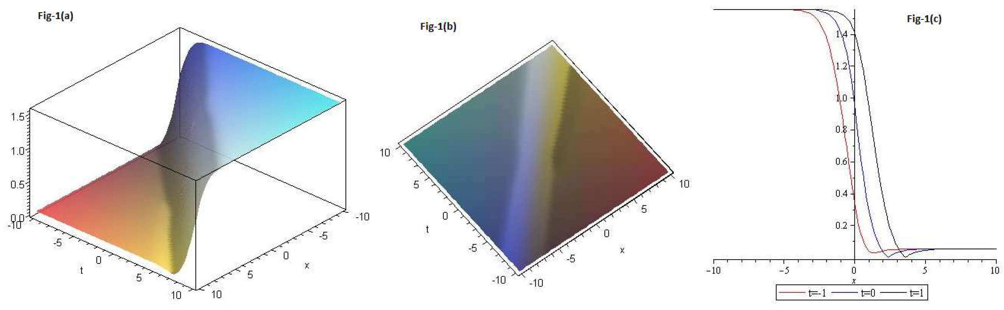
We draw plots for Eq.(13); in Figure 1. 1(a) 3D, 1(b) contour and 1(c) 2D for $-10\le t\le 10$ and $-10\le x\le 10$. Red curve is for $t=-1$, blue curve is for $t=0$ and black curve is for $t=1$ with $d=5,{\beta }_1=0.5,{\beta }_0=0.3,{\rm Y}=1,\delta =1,\lambda =-1,\rho =0.5,\theta =0.5,\alpha =0.8,$.

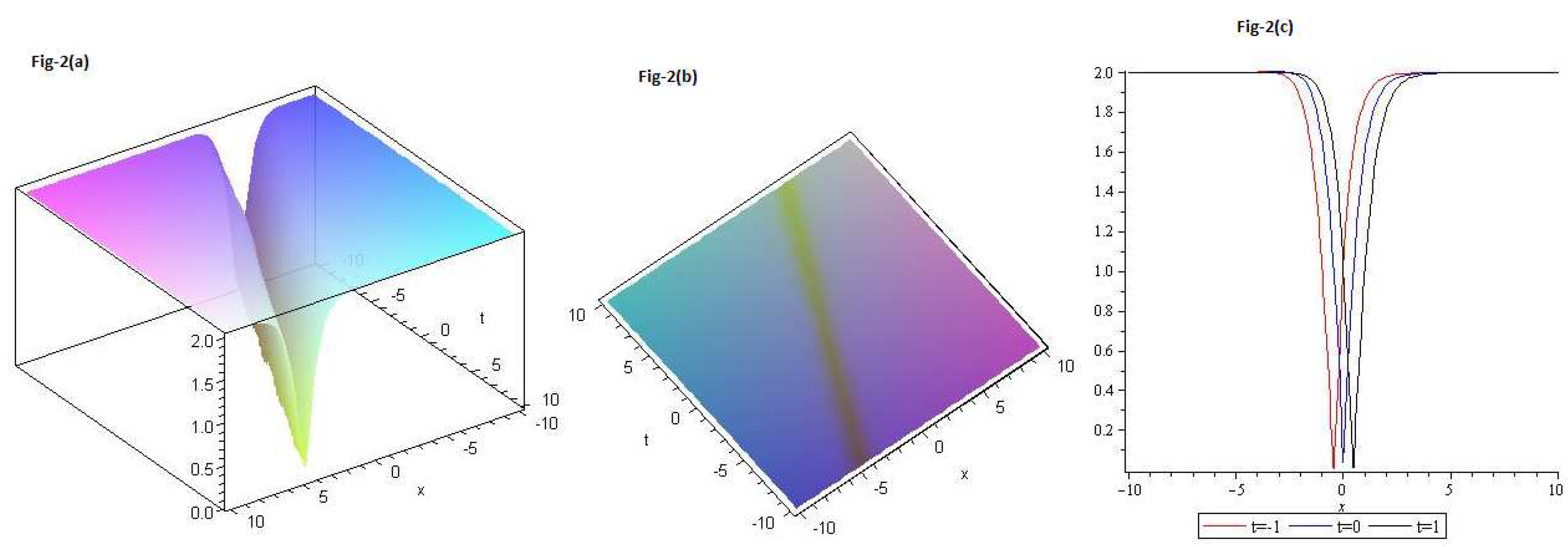
We draw plots for Eq.(36); in Figure 2. 2(a) 3D, 1(b) contour and 2(c) 2D for $-10\le t\le 10$ and $-10\le x\le 10$. Red curve is for $t=-1$, blue curve is for $t=0$ and black curve is for $t=1$ with ${\rm Y}=1,\delta =0.5,\eta =-1,\lambda =-1,\rho =0.5,\theta =0.5,\alpha =0.8,$.

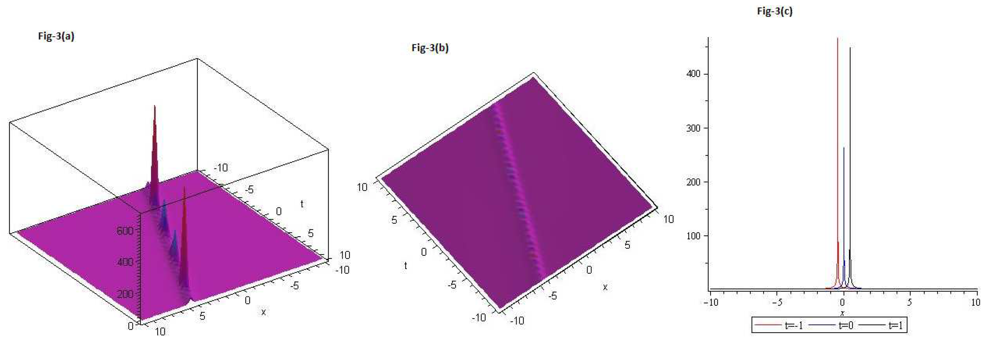
We draw plots for Eq.(37); in Figure 3. 3(a) 3D, 3(b) contour and 3(c) 2D for $-10\le t\le 10$ and $-10\le x\le 10$. Red curve is for $t=-1$, blue curve is for $t=0$ and black curve is for $t=1$ with ${\rm Y}=1,\delta =0.5,\eta =-1,\lambda =-1,\rho =0.5,\theta =0.5,\alpha =0.8,$.

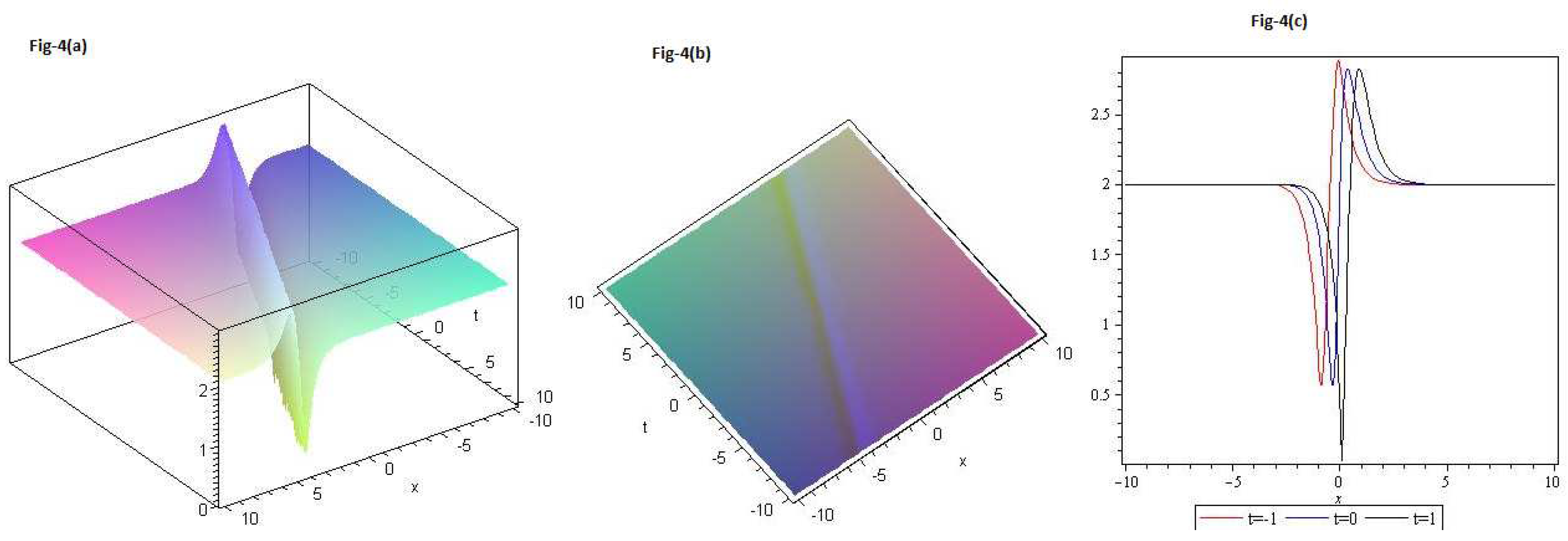
We draw plots for Eq.(38); in Figure 4. 4(a) 3D, 4(b) contour and 4(c) 2D for $-10\le t\le 10$ and $-10\le x\le 10$. Red curve is for $t=-1$, blue curve is for $t=0$ and black curve is for $t=1$ with ${\rm Y}=1,\delta =0.5,\eta =-1,\lambda =-1,\rho =0.5,\theta =0.5,\alpha =0.8,$.

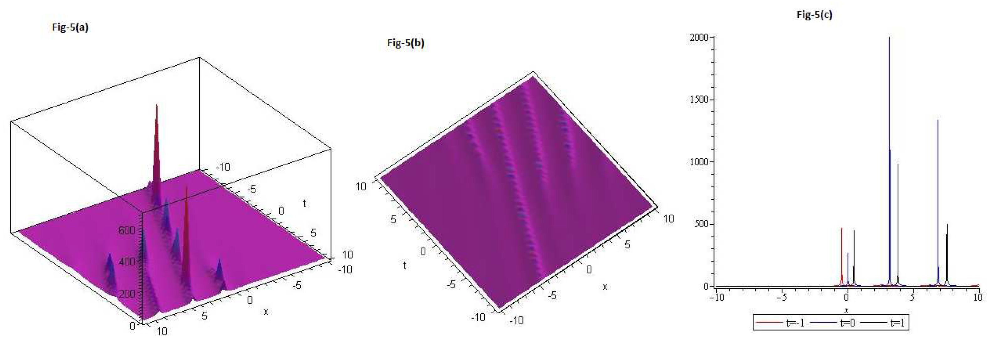
We draw plots for Eq.(42) in Figure 5. 5(a) 3D, 5(b) contour and 5(c) 2D for $-10\le t\le 10$ and $-10\le x\le 10$. Red curve is for $t=-1$, blue curve is for $t=0$ and black curve is for $t=1$ with ${\rm Y}=1,\delta =0.5,\eta =1,\lambda =-1,\rho =0.5,\theta =0.5,\alpha =0.8,$.

6. Conclusions

We are succeed to attain new soliton solutions to the M-fractional (1+1)-dimensional non-linear Westervelt model with the help of ${exp}_a$ function technique and modified simplest equation technique. Some of the gained results are represented graphically through Maple tool. The solutions achieved are helpful for the future study of this model. At the end, the techniques applied in our work are straight forward, reliable and fruitful to handle the other FPDEs.

References

- Bilal, Muhammad and Ahmad, Jamshad and others; New exact solitary wave solutions for the 3D-FWBBM model in arising shallow water waves by two analytical methods, Results in Physics, 25, 104230, (2021). [CrossRef]
- Alshahrani, B and Yakout, HA and Khater, Mostafa MA and Abdel-Aty, Abdel-Haleem and Mahmoud, Emad E and Baleanu, Dumitru and Eleuch, Hichem; Accurate novel explicit complex wave solutions of the (2+ 1)-dimensional Chiral nonlinear Schrödinger equation, Results in Physics, 23, 104019, (2021). [CrossRef]
- Bibi, Sadaf and Ahmed, Naveed and Khan, Umar and Mohyud-Din, Syed Tauseef; Some new exact solitary wave solutions of the van der Waals model arising in nature, Results in Physics, 9, 648–655, (2018). [CrossRef]
- Hafez, Mohammad Golam and Alam, Md Nur and Akbar, M Ali; Exact traveling wave solutions to the Klein–Gordon equation using the novel (G′/G)-expansion method, Results in Physics, 4, 177–184, (2014). [CrossRef]
- Seadawy, Aly R and Alamri, Sultan Z; Mathematical methods via the nonlinear two-dimensional water waves of Olver dynamical equation and its exact solitary wave solutions, Results in Physics, 8, 286–291, (2018). [CrossRef]
- Zafar, Asim and Ali, Khalid K and Raheel, Muhammad and Nisar, Kottakkaran Sooppy and Bekir, Ahmet; Abundant M-fractional optical solitons to the pertubed Gerdjikov–Ivanov equation treating the mathematical nonlinear optics, Optical and Quantum Electronics, 54, 1, 25, (2022). [CrossRef]
- Raheel, M and Zafar, Asim and Inc, Mustafa and Tala-Tebue, E; Optical solitons to time-fractional Sasa-Satsuma higher-order non-linear Schrödinger equation via three analytical techniques, Optical and Quantum Electronics, 55, 4, 307, (2023). [CrossRef]
- Chen, Zhuoxun and Manafian, Jalil and Raheel, Muhammad and Zafar, Asim and Alsaikhan, Fahad and Abotaleb, Mostafa; Extracting the exact solitons of time-fractional three coupled nonlinear Maccari’s system with complex form via four different methods, Results in Physics, 36, 105400, (2022). [CrossRef]
- Zafar, Asim and Raheel, M and Hosseini, Kamyar and Mirzazadeh, Mohammad and Salahshour, Soheil and Park, Choonkil and Shin, Dong Yun; Diverse approaches to search for solitary wave solutions of the fractional modified Camassa–Holm equation, Results in Physics, 31, 104882, (2021). [CrossRef]
- Razzaq, Waseem and Habib, Mustafa and Nadeem, Muhammad and Zafar, Asim and Khan, Ilyas and Mwanakatwea, Patrick Kandege; Solitary Wave Solutions of Conformable Time Fractional Equations Using Modified Simplest Equation Method, Complexity, 2022, (2022). [CrossRef]
- Razzaq, Waseem and Zafar, Asim and Akbulut, Arzu; The modified simplest equation procedure for conformable time-fractional Boussinesq equations, International Journal of Modern Physics B, 36, 17, 2250095, (2022). [CrossRef]
- Ghazanfar, Sidra and Ahmed, Nauman and Iqbal, Muhammad Sajid and Akgül, Ali and Bayram, Mustafa and De la Sen, Manuel; Imaging ultrasound propagation using the Westervelt equation by the generalized Kudryashov and modified Kudryashov methods, Applied Sciences, 12, 22, 11813, (2022). [CrossRef]
- Shaikh, Tahira Sumbal and Baber, Muhammad Zafarullah and Ahmed, Nauman and Iqbal, Muhammad Sajid and Akgül, Ali and El Din, Sayed M; Acoustic wave structures for the confirmable time-fractional Westervelt equation in ultrasound imaging, Results in Physics, 49, 106494, (2023). [CrossRef]
- Tukur Abdulkadir Sulaiman, Gulnur Yel and Hasan Bulut; M-fractional solitons and periodic wave solutions to the Hirota- Maccari system, Modern Physics Letters B, 1950052, (2019). [CrossRef]
- J. Vanterler D A C. Sousa, and E. Capelas D E Oliveira; A new truncated M-fractional derivative type unifying some fractional derivative types with classical properties, International Journal of Analysis and Applications, 16, 1 , 83-96, (2018). [CrossRef]
- A. T. Ali and E.R. Hassan, General Expa-function method for nonlinear evolution equations, Applied Mathematics and Computation, 217(2) 451-459, (2010). [CrossRef]
- E.M.E. Zayed and A.G. Al-Nowehy, Generalized kudryashov method and general expa function method for solving a high order nonlinear schrödinger equation, J. Space Explor, 6, 1-26, (2017).
- K. Hosseini, Z. Ayati and R. Ansari, New exact solutions of the Tzitzéica-type equations in non-linear optics using the expa function method, Journal of Modern Optics, 65(7), 847-851,(2018). [CrossRef]
- A. Zafar, The expa function method and the conformable time-fractional KdV equations, Nonlinear Engineering, 8, 728-732, (2019). [CrossRef]
Disclaimer/Publisher’s Note: The statements, opinions and data contained in all publications are solely those of the individual author(s) and contributor(s) and not of MDPI and/or the editor(s). MDPI and/or the editor(s) disclaim responsibility for any injury to people or property resulting from any ideas, methods, instructions or products referred to in the content. |
© 2023 by the authors. Licensee MDPI, Basel, Switzerland. This article is an open access article distributed under the terms and conditions of the Creative Commons Attribution (CC BY) license (http://creativecommons.org/licenses/by/4.0/).
Copyright: This open access article is published under a Creative Commons CC BY 4.0 license, which permit the free download, distribution, and reuse, provided that the author and preprint are cited in any reuse.