Submitted:
26 September 2023
Posted:
27 September 2023
You are already at the latest version
Abstract
The effects of wastewater step-feeding on the performance of Horizontal Subsurface Flow Constructed Wetlands (HSF CWs) are numerically investigated. The purpose is to check if this alternative feeding technique increases the ability of HSF CWs to remove pollutants. Two methodologies are used: Initially, the Tanks-In-series (TIS) methodology, based on Finite Volume Method (FVM), is analyzed by using the volumetric degradation coefficient λ. In this case the operation of CW is similar with a series of Continuous Stirred-Tank Reactors (CSTR), under steady conditions. Then, the Step-Feeding (SF) procedure is presented, when the CW is operated like a Plug Flow Reactor (PFR). The results show that the SF procedure does not improve the performance of HSF CWs on removing Biochemical Oxygen Demand (BOD), operating under Mediterranean conditions.
Keywords:
step-feeding
; constructed wetlands
; Tanks-In-Series
; Continuous Stirred-Tank Reactor
; Plug Flow Reactor
; numerical investigation
; Biochemical Oxygen Demand
1. Introduction
The wastewater treatment is one of the main problems that should be solved in order to secure the protection of the environment and the public health, especially in small cities and settlements where the construction and operation of modern wastewater treatment units is difficult to exist. An effective, economic and ecological solution for this problem is the construction and operation of Constructed Wetlands (CWs) [1,2,3]. As these systems are becoming increasingly popular in the last 25 years, especially in developing countries, it is important to investigate if the use of alternative feeding techniques could have positive or negative effect on their performance. One of these techniques is the step-feeding of the wastewater [4,5,6].
“Step-feeding” (SF) describes the case when the wastewater is not introduced totally at the inlet of the CW, but it is splitted at several points along the flow path in a gradational way. Most of the studies that have been realized concerning the SF procedure in Vertical Flow (VF) CWs [7,8,9,10,11,12,13]. Less studies are available about the implementation of SF technique in Horizontal Subsurface Flow (HSF) CWs [14,15], by using experiments [16] or computer codes [17]. A briefly description of these studies is presented in next paragraph.
The economical cost for the construction and operation of a CW facility could be useless and have a negative impact, if the results don’t provide a sustainable solution. It means that the inlet contaminated wastewater must have at the outlet, after its “treatment” inside the CW, zero (or almost zero) concentration. The operation could be sustainable also in the case that the outlet concentration is significant smaller, in comparison with the inlet concentration. Usually the CW operation provides positive results, as the outlet wastewater is cleaner than the inlet quantity.
Alternative feeding techniques, like wastewater step-feeding or effluent recirculation, are used in praxis in order to succeed a better result. But, as presented with details in the present study, sometimes SF does not improve the performance of a CW on a pollutant removal, and in this case the procedure should not be selected. The key factors usually are operation characteristics, like environmental parameters, type of pollutant, dimensions of CW exc.
In the present study, it is numerically investigated if SF could increase the ability of HSF CWs to remove Biochemical Oxygen Demand (BOD), which is one of the main pollutants monitored in municipal wastewaters. This investigation is realized for pilot-scale HSF CWs, which were constructed and operated under Mediterranean conditions. The results of the present study could be an important tool in order to check the sustainability of these systems, when they operate under these conditions. They also provide the possibility to avoid the (construction and operation) cost, if the conclusion is that the SF procedure does not really improve the performance of CWs.
2. The Numerical Formulation of Step-feeding
The problem of SF is formulated for the case of a pilot-scale HSF CW, which is presented in Figure 1.
Totally five similar HSF CWs were constructed and are still in operation, in the facilities of Laboratory of Ecological Engineering and Technology, Department of Environmental Engineering, Democritus University of Thrace, Xanthi, Greece. The dimensions of each CW tank is 3 m in length, 0.75 m in width and 1 m in depth, while the thickness of the porous media is 0.45 m.
A different combination of vegetation and porous medium is appeared in each tank. The types of porous materials were Medium Gravel (MG), Fine Gravel (FG) and Cobbles (CO). The tanks were planted with common Reeds (phragmites australis - R) or Cattails (typha latifolia – C), while one tank was kept unplanted (Z). Therefore, the symbols of the five tanks were: MG-R, MG-C, MG-Z, FG-R and CO-R. The units were equipped with vertical perforated plastic pipes (50 mm diameter each), which could be used in praxis during the SF procedure for the introduction of the wastewater at several points among the length (each pipe per 1 m), as shown in Figure 1.
The main operational characteristics are presented in Table 1, for a total operation period of two years. For each CW tank and for the used values of Hydraulic Residence Time HRT (6, 8, 14 and 20 days), the experimental values of porosity ε, hydraulic conductivity K, volume of porous material Vp, average temperature Tav, inlet and outlet concentrations of the pollutant (BOD), Cin and Cout respectively, and first-order decay coefficient λ, are presented. A more detailed description for the calculation and explanation for each one of these parameters is given by [18]. The impact of the size of porous materials is obvious in the values of hydraulic conductivity, especially between the tanks FG-R and CO-R.
The total inflowing wastewater flow rate Q = Qin, in [L/day], is distributed in three inflowing points along the CW tank: x0 = 0, x1 = 1 m and x2 = 2 m. The following equations give the inflowing wastewater flow rates for each one of these points:
where x, y, z are the corresponding percentages of Q in each position; therefore, they fulfill the condition:
In order to ensure saturated positive flow from the inlet to the outlet, it should be:
When the SF procedure is present during the operation of the wetlands, i.e., x#0, y#0 and z#0, the aim is to determine the optimal values of these percentages in order to minimize the concentration of the pollutant at the outlet Cout, in [mg/L]. Then, this value should be compared with the corresponding outlet concentration for the case that CW is operated without SF, i.e., x = 1 and y = z = 0. The results of this comparison give the answer if the performance of the tank was increased or decreased, by using the SF procedure. The performance R, in [%], is given by the following equation:
3. Analysis by using the TIS Methodology
For the numerical investigation of the problem, first the Tanks-In-Series (TIS) methodology is used [19], which is based on Finite Volume Method [20,21]. It is considered that the wetlands are operated as Continuous Stirred-Tank Reactors (CSTR), under steady conditions, and the volumetric degradation coefficient λ is used. According to the experimental procedure [16], the tank is splitted in three equal cells (Figure 2), with corresponding volumetric degradation coefficients λ1, λ2 and λ3.
The above cells have equal volume, which is:
where Vp = εLWd; L is the length of the CW, in [m]; W is the width of the CW, in [m]; and d is the depth of the porous material, in [m].
As shown in Figure 2, the operation of the above system begins with the entering flow rate Q1 at the inlet of the first cell. The outlet flow rate of the first cell Q1 is mixed with the entering flow rate of the second cell Q2. Similarly, the outlet flow rate of the second cell Q1 +Q2 is mixed with the entering flow rate of the third cell Q3. Finally, at the end of the operation, the concentration Cout,3 is the outlet concentration of the system Cout which should be minimized.
The numerical formulation of the whole procedure is the following: For the first cell K1, the outlet concentration Cout,1 and the Hydraulic Residence Time HRT1 are:
The pollutant mass balance between the first and the second cell is used, in order to determine the inlet concentration Cin,2:
Thus, it is:
The equations (4a) and (4d) show:
Similarly, for the second cell K2, the outlet concentration Cout,2 and the Hydraulic Residence Time HRT2 are:
The pollutant mass balance between the second and the third cell is used:
Thus, the inlet concentration at the third cell Cin,3 is:
The equations (5a) and (5d) show:
Finally, for the third cell K3, the outlet concentration Cout,3 (which is the outlet concentration for the whole system Cout) and the Hydraulic Residence Time HRT3 are:
The main problem could be express numerically like this: Which are the optimal values of x,y,z in order to minimize the function: Cout = f (x,y,z)?
For operation without the SF technique, i.e., x = 1 and y = z = 0, and by considering that the volumetric degradation coefficient is the same for all the three cells (λ1=λ2=λ3=λ), the equation (6a) gives the well-known TIS equation [2,12]:
and the Hydraulic Residence Time for the whole system HRT is:
4. Analysis by using the PFR Methodology
The pilot-scale HSF CWs could be considered that they operate like Plug Flow Reactors (PFR). It means that the contribution of the dispersion during the operation of the tanks is negligible. By following the same steps with previous paragraph, and for λ1=λ2=λ3=λ, the inlet and outlet concentrations are determined.
Thus, for the first cell K1:
Similarly, for the cell K2:
Finally, for the last cell K3:
5. Results and Discussion
5.1. Numerical Example
By using typical average values for the main parameters, a numerical example is presented below in order to check if the SF procedure increases or decreases the performance of the HSF CWs on the BOD removal. Four scenarios are investigated and the outlet concentration (Cout) for each one of these scenarios is compared with the corresponding outlet concentration when the wetlands are operating without SF. The average values for the main parameters, according to available experimental data [18], are: Qin = Q = 40 L/day, Vp = 360 L, HRT = 9 days and λ1 = λ2 = λ3 = λ = 0.15 day-1.
First, the TIS methodology is followed. According to equation (3), it is: V1 = V2 = V3 = 120 L. By using the equations (1) and (4) - (6), the values of inlet concentrations, outlet concentrations and Hydraulic Residence Time are:
Cell K1:
Cell K2:
Cell K3:
Thus, by following the limitations of Equations (1d) and (1e), the purpose is to determine the optimal values of x,y,z which minimize the function Cout = f(x,y,z) of the above Equation (12).
Except the scenario (A), in which the CWs are operated without SF (x = 1 and y = z = 0), four more scenarios are investigated:
(B) The wastewater is introduced at two inflowing points among the HSF CW length: 80% at x0 = 0 and 20% at x1 = 1 m, i.e., x = 0.80, y = 0.20 and z = 0.
(C) The wastewater is introduced at two inflowing points among the HSF CW length: 60% at x0 = 0 and 40% at x1 = 1 m, i.e., x = 0.60, y = 0.40 and z = 0.
(D) The wastewater is introduced at three inflowing points among the HSF CW length: 60% at x0 = 0, 25% at x1 = 1 m and 15% at x2 = 2 m, i.e., x = 0.60, y = 0.25 and z = 0.15.
(E) The wastewater is introduced at three inflowing points among the HSF CW length: 33.33% at x0 = 0, 33.33% at x1 = 1 m and 33.33% at x2 = 2 m, i.e., x = y = z = 0.333.
The introduction of the above values of x,y,z in Equation (12) gives these outlet concentration for each scenario: Cout,A = 0.3280Cin, Cout,B = 0.3386Cin, Cout,C = 0.3533Cin, Cout,D = 0.3708Cin and Cout,E = 0.4255Cin. Therefore, the outlet concentration in minimum for the scenario (A), i.e., when the CW operates without SF.
Similarly, the PFR methodology is used. For the same values of Q, VP, HRT and λ, the equations (1) and (8)-(10) give the following results:
Cell K1:
Cell K2:
Cell K3:
Again, the optimal values x,y,z which minimize the function Cout = f(x,y,z) of Equation (13) should be determined, when the limitations of equations (1d) and (1e) are followed.
The above SF scenarios (A)-(E), are investigated. In this case, of the outlet concentrations are: Cout,A = 0.2592Cin, Cout,B = 0.2667Cin, Cout,C = 0.2779Cin, Cout,D = 0.2959Cin and Cout,E = 0.3980 Cin. These results show that for both methodologies the best performance of CW, which means the minimum values of Cout, appear when the wetlands operate without the SF procedure.
The above results are presented in Table 2, which shows the relationship between the Cin and Cout concentrations, for each methodology and SF scenario.
For the numerical proposed result, the data of Table 2 and the Equation (2) are used. Table 3 provides, for each methodology (TIS and PFR) the values of the performance of the HSF CW, for the SF scenarios (A)-(E). These values were calculated for a typical average value of inlet concentration Cin = 360 mg BOD/L, by using the equations (2), (12) and (13).
5.2. Discussion and Comparison with other Studies
For both methodologies (TIS and PFR), the results show that the minimum values of outlet concentration Cout (therefore, the maximum performance on BOD removal) were found for the scenario according to which the CWs are operating without SF. This confirms that this procedure does not increase the performance of the HSF CWs, at least for wetlands operation with similar Mediterranean conditions with the present study. On the contrary, when the number of inlet points of the wastewater among the CW tank is increased to more than one inlet point, see scenarios (D) and (E) of previous paragraph, the ability of the wetlands to remove BOD becomes lower. The main explanation of this is that the parts of the effluent which enters in the points x1 = 1 m and x2 = 2 have lower HRT; thus, the total time of the operation of the HSF CW is smaller.
The conclusion of the present work confirms the results of a relative computational study [17]: For the same pilot-scale HSF CWs, and by using the computer code Visual MODFLOW, it was proved that SF acts negatively on the performance of these tanks to remove BOD. Schematically, a part of the results from this computational research is shown in Figure 3. This diagram concerns the HSF CW tank which contains medium gravel as porous material and it is planted with common reed (Phragmites australis). The values of the main parameters are: HRT = 14 days, Cin = 360 mg BOD/L, λ = 0.06 day-1 and ε = 0.38. For the SF procedure, the scenario (D) is investigated, i.e., x=0.60, y=0.25 and z=0.15.
In Figure 3, the outlet BOD concentration without SF is Cout,A = 8.42 mg/L, while with SF is sensibly higher, Cout,D = 17.47 mg/L. The inequalities (4e) and (5e) could explain the occurrence of the “leaps” in the longitudinal concentration distribution profile, at the feeding positions x1 = 1 m and x2 = 2 m.
Stefanakis et al. [16] also presented an experimental procedure for the same tanks and they have investigated the above SF scenarios (D) and (E), for the pollutants of BOD, Chemical Oxygen Demand (COD) and TKN (Total Kjeldahl Nitrogen). While an agreement has been observed between these experimental results and the numerical results of the present work concerning the scenario (E), i.e., x = y = z = 0.333, a small difference is appeared about the scenario (D), i.e., x = 0.60, y = 0.25 and z = 0.15. Stefanakis et al. [16] concluded that the SF slightly increases the performance of the HSF CWs on BOD removal, for this scenario. It can be explained by the fact that the experiments were realized during the summer months, where the ability of CWs to remove pollutants is always bigger, due to high temperatures and the growth of the plants.
Li et al. [15] investigated experimentally the removal of COD, Total Nitrogen (TN) and ammonium nitrogen (NH4+-N). As the results show, the HRT could effect the effectiveness of SF procedure. Especially for COD and NH4+-N removal, the SF procedure acted negatively on CW performances for low HRT = 5 days, but on the contrary it increased the performance of the wetlands for higher HRT = 8.4 days. Concerning the TN, SF seems to increase significantly the performance of HSF CWs, but the removal of nitrogen requires special investigation as it is governed by the phenomenon of adsorption.
On contrary with HSF CWs, more studies have been realized concerning SF in VF CWs. Fan et al. [12] investigated a SF scenario where half wastewater is introduced at the inlet and another half at the middle of VF CW, an operation similar with the SF scenario (F) of the present study. The results showed that the COD removal was increased slightly, while the increase of the performance on TN removal was remarkable. Hu et al. [6] succeed to show higher performance on nitrogen removal on VF CWs for the SF scenario (B), i.e., x = 0.80, y = 0.20 and z = 0.
Moreover, Khajah et al. [7] investigated in a VF CW the effects of SF concerning COD and TN removal, for the scenarios (B) and (C). The performance was increased concerning COD, but remained stable for TN removal. Similarly, positive effects on the ability of VF CWs to remove pollutant was recorder by Saeed et al. [8], concerning BOD and Total Phosphorus (TP) removal for the SF scenario (F).
Wang et al. [10] did not conclude an important effect of SF on organics removal for the scenarios (E) and (F), as the performance with and without the SF procedure remained almost stable. Finally, Torrijos et al. [9] investigated the effects of SF on the performance of a hydrid system, which included both a HSF and a VF CW. The removal of COD was increased from 96% to 99% for the SF scenario (F).
The following Table 4 presents the results of all these studies. The performance of the HSF and VF CWs for various pollutants and for all the different SF scenarios described in the previous paragraphs are shown. These results show that the SF procedure generally increases the ability of VF CWs to remove pollutants, whereas has a negative effect on the performance of HSF CWs. In any case, the environmental operation parameters (like temperature, rainfall, growth of plants) could give non stable results, especially to the comparison between experimental researches.
6. Conclusions
A numerical investigation, based on TIS and PFR methodologies, was presented concerning the effects of wastewater step-feeding on the removal efficiency of HSF CWs. Numerical examples confirmed that this feeding technique acts negatively on the performance of these wetlands, especially when more than two inlet positions along the CW for the wastewater are chosen. Thus, this operation technique does not improve the ability of HSF CWs to remove pollutants, at least when they operate under Mediterranean conditions. Therefore, the operation of (pilot-scale or full scale) CWs by using the SF technique is not recommended, at least for facilities with similar characteristics with the present study.
Moreover, a comparison with other similar studies has been realized and showed the importance, not only of the wastewater direction (HSF or VF CWs), but also of the operational characteristics of the CWs (kind of vegetation and porous material, climatic parameters, hydraulic residence time, type of pollutant). The effect of these characteristics on SF techniques is important to be investigated in futural relevant studies. As a general conclusion, the results of the present study could be useful for better understanding of the use of alternative feeding techniques (like wastewater step-feeding or recirculation of the effluent) in constructed wetlands.
References
- Vymazal, J.; Zhao, Y.; Mander, U. Recent research challenges in constructed wetlands for wastewater treatment: A review. Ecol. Eng. 2021, 169, 106318. [Google Scholar] [CrossRef]
- Parde, D.; Patwa, A.; Shukla, A.; Vijay, R.; Killedar, D.J.; Kumar, R. A review of constructed wetland on type, treatment and technology of wastewater. Environ. Technol. Innov. 2021, 21, 101261. [Google Scholar] [CrossRef]
- Moshiri, G.A. Constructed Wetlands for Water Quality Improvement; CRC Press: Boca Raton, FL, USA, 2020. [Google Scholar]
- Varma, M.; Gupta, A.K.; Ghosal, P.S.; Majumder, A. A review on performance of constructed wetlands in tropical and cold climate: Insights of mechanism, role of influencing factors, and system modification in low temperature. Sci. Total Env. 2021, 755, 142540. [Google Scholar] [CrossRef] [PubMed]
- Meng, P.; Pei, H.; Hu, W.; Shao, Y.; Li, Z. How to increase microbial degradation in constructed wetlands: Influencing factors and improvement measures. Bioresource Technol. 2014, 157, 316–326. [Google Scholar] [CrossRef]
- Saeed, T.; Sun, G. A review on nitrogen and organics removal mechanisms in subsurface flow constructed wetlands: Dependency on environmental parameters, operating conditions and supporting media. J. Environ. Manage. 2012, 112, 429–448. [Google Scholar] [CrossRef] [PubMed]
- Khajah, M.; Bydalek, F.; Babatunde, A.O.; Al-Matouq, A.; Wenk, J.; Webster, G. Nitrogen removal performance and bacterial community analysis of a multistage step-feeding tidal flow constructed wetland. Front. Water 2023, 5, 1128901. [Google Scholar] [CrossRef]
- Saeed, T.; Miah, M.J.; Khan, T.; Ove, A. Pollutant removal employing tidal flow constructed wetlands: Media and feeding strategies. Chem. Eng. J. 2020, 382, 122874. [Google Scholar] [CrossRef]
- Torrijos, V.; Ruiz, I.; Soto, M. Effect of step-feeding on the performance of lab-scale columns simulating vertical flow-horizontal flow constructed wetlands. Environ. Sci. Pollut. R. 2017, 24, 22649–22662. [Google Scholar] [CrossRef] [PubMed]
- Wang, Z.; Huang, M.; Qi, R.; Fan, S.; Wang, Y.; Fan, T. Enhanced nitrogen removal and associated microbial characteristics in a modified single-stage tidal flow constructed wetland with step-feeding. Chem. Eng. J. 2017, 314, 291–300. [Google Scholar] [CrossRef]
- Shen, L.; Wu, J.; Zhong, F.; Xiang., D.; Cheng, S. Effect of step feeding on the performance of multi-stage vertical flow constructed wetland for municipal wastewater treatment. J. Lake Sci. 2017, 29(5), 1084–1090. [Google Scholar]
- Fan, J.; Liang, S.; Zhang, B.; Zhang, J. Enhanced organics and nitrogen removal in batch-operated vertical flow constructed wetlands by combination of intermittent aeration and step feeding strategy. Environ. Sci. Pollut. R. 2013, 20, 2448–2455. [Google Scholar] [CrossRef] [PubMed]
- Hu, Y.S.; Zhao, Y.Q.; Zhao, X.H.; Kumar, J.L.G. Comprehensive analysis of step-feeding strategy to enhance biological nitrogen removal in alum sludge-based tidal flow constructed wetlands. Bioresource Technol. 2012, 111, 27–35. [Google Scholar] [CrossRef] [PubMed]
- Patil, S.; Chakraborty, S. Effects of step-feeding and intermittent aeration on organics and nitrogen removal in a horizontal subsurface flow constructed wetland. J. Environ. Sci. Heal. A 2017, 52(4), 403–412. [Google Scholar] [CrossRef] [PubMed]
- Li, F.; Lu, L.; Zheng, X.; Ngo, H.H.; Liang, S.; Guo, W.; Zhang, X. Enhanced nitrogen removal in constructed wetlands: Effects of dissolved oxygen and step-feeding. Bioresource Technol. 2014, 169, 395–402. [Google Scholar] [CrossRef] [PubMed]
- Stefanakis, A.I.; Akratos, C.S.; Tsihrintzis, V.A. Effect of wastewater step-feeding on removal efficiency of pilot-scale horizontal subsurface flow constructed wetlands. Ecol. Eng. 2011, 37(3), 431–443. [Google Scholar] [CrossRef]
- Liolios, K.A.; Moutsopoulos, K.N.; Tsihrintzis, V.A. Modelling alternative feeding techniques in HSF constructed wetlands. Environ. Proces. 2016, 3(1), 47–63. [Google Scholar] [CrossRef]
- Liolios, K.A.; Moutsopoulos, K.N.; Tsihrintzis, V.A. Modeling of flow and BOD fate in horizontal subsurface flow constructed wetlands. Chem. Eng. J. 2012, 200-202, 681–693. [Google Scholar] [CrossRef]
- Stephenson, R.; Sheridan, C.; Kappelmeyer, U. A curve-shift technique for the use of non-conservative organic tracers in constructed wetlands.). Sci. Total Env. 2021, 752, 141818. [Google Scholar] [CrossRef] [PubMed]
- Moukalled, F.; Mangani, L.; Darwish, M. The Finite Volume Method in Computational Fluid Mechanics; Springer International Publishing: Cham, Switzerland, 2016. [Google Scholar]
- Bear, J.; Cheng, A.H.D. Modeling Groundwater Flow and Contaminant Transport; Springer Dordrecht Heidelberg: New York, USA, 2010. [Google Scholar]
Figure 1.
Schematic diagram of the HSF CW tank.
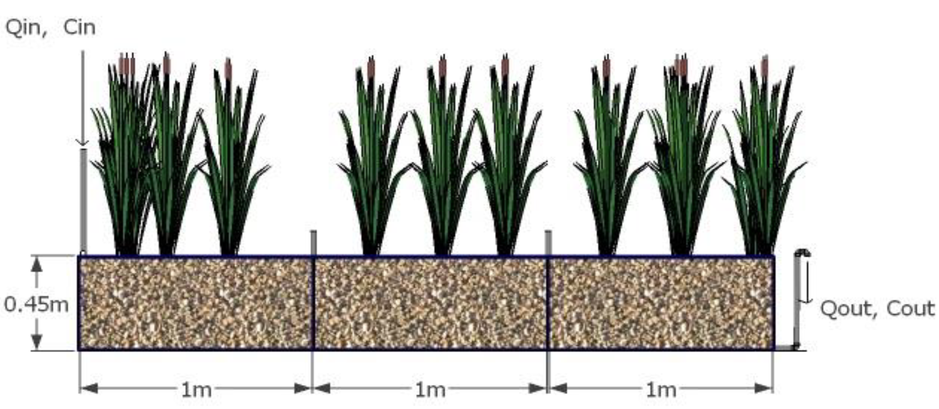
Figure 2.
TIS system of constructed wetlands.
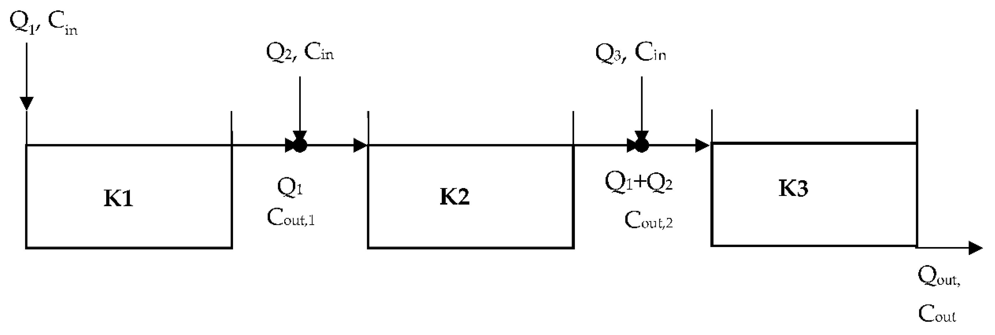
Figure 3.
Longitudinal concentration distribution profile of concentration C/Cin among the HSF CW, for the scenarios (A): “SFS 100-0-0” and (D): SFS 60-25-15.
Figure 3.
Longitudinal concentration distribution profile of concentration C/Cin among the HSF CW, for the scenarios (A): “SFS 100-0-0” and (D): SFS 60-25-15.
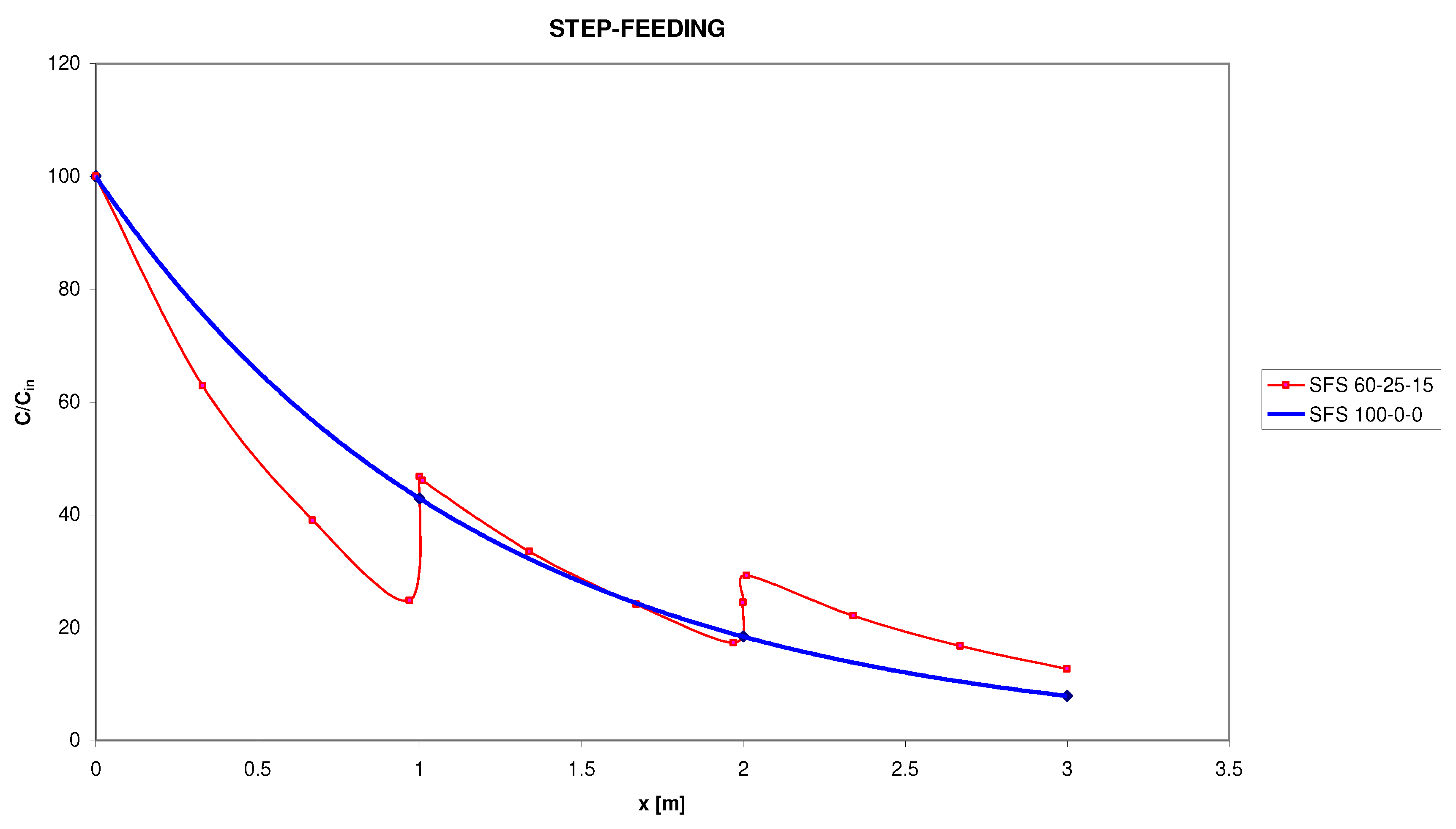

Table 1.
Operation characteristics of HSF CWs.
| CW tank | HRT [days] | ε [%] |
Κ [m/sec] |
Vp [m3] |
Tav [oC ] |
Cin [mg/L] |
Cout [mg/L] |
λ [day-1] |
|---|---|---|---|---|---|---|---|---|
| MG-R | 6 8 14 20 |
0.35 | 0.7196 0.7640 0.9743 0.7196 |
0.3544 0.3594 0.3848 0.3544 |
5.7 11.8 18.7 22.4 |
321.5 333.0 332.0 345.3 |
141.8 87.7 60.9 48.3 |
0.1212 0.1992 0.2546 0.3852 |
| 0.355 0.38 0.35 | ||||||||
| MG-C | 6 | 0.33 | 0.5620 | 0.3341 | 25.7 | 327.0 | 26.0 | 0.3852 |
| 8 | 0.335 | 0.5980 | 0.3392 | 4.5 | 350.0 | 124.0 | 0.1155 | |
| 14 20 |
0.34 0.33 |
0.6366 0.5620 |
0.3443 0.3341 |
8.8 13.1 |
358.6 348.5 |
72.4 50.8 |
0.1799 0.2178 |
|
| MG-Z | 6 8 14 20 |
0.37 0.37 0.37 0.37 |
0.9120 0.9120 0.9120 0.9120 |
0.3746 0.3746 0.3746 0.3746 |
16.3 19.2 11.2 17.9 |
380.0 373.7 372.0 358.7 |
34.3 22.6 65.3 40.3 |
0.2740 0.3217 0.1126 0.1426 |
| FG-R | 6 8 14 20 |
0.29 0.29 0.31 0.29 |
0.0199 0.0199 0.0262 0.0199 |
0.2936 0.2936 0.3139 0.2936 |
21.2 8.7 13.8 16.3 |
461.5 355.8 323.3 364.3 |
30.7 45.5 22.9 34.8 |
0.1784 0.0923 0.1210 0.1066 |
| CO-R | 6 8 14 20 |
0.28 0.28 0.28 0.28 |
3.8710 3.8710 3.8710 3.8710 |
0.2835 0.2835 0.2835 0.2835 |
21.9 5.7 11.8 18.7 |
381.4 321.5 333.0 332.0 |
35.0 141.8 87.7 60.9 |
0.1085 0.1212 0.1992 0.2546 |
Table 2.
Impact of SF on the relationship between Cin and Cout.
| Step-feeding scenario | TIS methodology | PFR methodology |
|---|---|---|
| (A) | Cout = 0.3280Cin | Cout = 0.2592Cin |
| (B) | Cout = 0.3386Cin | Cout = 0.2667Cin |
| (C) | Cout = 0.3533Cin | Cout = 0.2779Cin |
| (D) | Cout = 0.3708Cin | Cout = 0.2959Cin |
| (E) | Cout = 0.4255Cin | Cout = 0.3980 Cin |
Table 3.
Performance of HSF CW on BOD removal, with and without SF, for TIS and PFR methodologies.
| Step-feeding scenario | HSF CW performance [%] for TIS method |
HSF CW performance [%] for PFR method |
|---|---|---|
| (A) | 67.20 | 74.08 |
| (B) | 66.14 | 73.33 |
| (C) | 64.67 | 72.21 |
| (D) | 62.92 | 73.33 |
| (E) | 57.45 | 60.20 |
Table 4.
Performance [%] of HSF and VF CWs for various pollutants and SF scenarios.
| Reference | CW type |
Pollutant | Step-feeding scenario | |||||
|---|---|---|---|---|---|---|---|---|
| (A) | (B) | (C) | (D) | (E) | (F) | |||
| Stefanakis et al. [16] (HRT = 6 days) |
BOD | 84.2 | — | — | 88.7 | — | — | |
| HSF | COD | 82.7 | — | — | 87.4 | — | — | |
| TKN | 76.5 | — | — | 75.5 | — | — | ||
| Stefanakis et al. [16] (HRT = 14 days) |
BOD | 89.4 | — | — | — | 83.3 | — | |
| HSF | COD | 89.4 | — | — | — | 84.0 | — | |
| NH4+-N | 71.8 | — | — | — | 38.5 | — | ||
| Liolios et al. [17] | HSF | BOD | 92.5 | 91.7 | 90.3 | 88.2 | 82.1 | — |
| Li et al. [15] (HRT = 5 days) |
COD | 87.2 | 67.8 | — | — | — | — | |
| HSF | NH4+-N | 99.0 | 93.5 | — | — | — | — | |
| TN | 55.5 | 60.6 | — | — | — | — | ||
| Li et al. [15] (HRT = 8.4 days) |
HSF | COD NH4+-N TN |
83.2 98.9 56.4 |
90.9 99.1 88.1 |
— — — |
— — — |
— — — |
— — — |
| Fan et al. [5] |
VF | COD TN |
88.0 44.0 |
— — |
— — |
— — |
— — |
97.0 82.0 |
| Hu et al. [6] | VF | TN | 85.0 | 90.2 | — | — | — | — |
| Khajah et al. [7] |
VF | COD TN |
75.0 73.5 |
94.0 70.0 |
90.0 75.0 |
— — |
— — |
— — |
| Saeed et al. [8] |
VF | BOD TP |
87.4 92.4 |
— — |
— — |
— — |
— — |
93.9 94.2 |
| Wang et al. [10] |
VF | BOD COD |
97.2 96.5 |
— — |
— — |
— — |
95.9 95.9 |
96.8 99.9 |
| Torrijos et al. [9] | HSF+VF | COD | 96.0 | — | — | — | — | 99.0 |
Disclaimer/Publisher’s Note: The statements, opinions and data contained in all publications are solely those of the individual author(s) and contributor(s) and not of MDPI and/or the editor(s). MDPI and/or the editor(s) disclaim responsibility for any injury to people or property resulting from any ideas, methods, instructions or products referred to in the content. |
© 2023 by the author. Licensee MDPI, Basel, Switzerland. This article is an open access article distributed under the terms and conditions of the Creative Commons Attribution (CC BY) license (http://creativecommons.org/licenses/by/4.0/).
Copyright: This open access article is published under a Creative Commons CC BY 4.0 license, which permit the free download, distribution, and reuse, provided that the author and preprint are cited in any reuse.


