
Submitted:
18 September 2023
Posted:
19 September 2023
You are already at the latest version
Abstract
The educational and play-related activities of children are proceeded mainly indoors in a kin-dergarten. The exposure of children to high concentrations of PM2.5 and CO2 indoors have leaded to various harmful effects and negatively impact educational outcomes in a kindergarten. Therefore, this study presents a numerical model of CO2 and PM2.5 concentration based on two classrooms in a kindergarten. Using this numerical model, we present different scenarios of oper-ating mechanical ventilation and air purifiers in kindergartens with the aim of optimizing for reducing the concentrations of CO2 and PM2.5. We found that the amount of ventilation required to maintain good air quality, per child, was approximately 20.4 m3/h. However, we also found that as the amount of ventilation increased, so did the concentration of indoor PM2.5; we found that this issue can be resolved through the use of a high-grade filter (i.e., a MERV 13 grade filter with a collection efficiency of 75%). This study provides a scientific basis for reducing PM2.5concentrations in kindergartens, while keeping CO2 levels low.
Keywords:
Kindergarten
; CO2
; PM2.5
; Mechanical Ventilation
; Indoor Air Quality
; Numerical model
= Indoor CO2 Concentration (ppm) =
(t) = Indoor PM2.5 Concentration (㎍/m3) =
= Outdoor CO2 Concentration (ppm)
= Outdoor PM2.5 Concentration (㎍/m3)
= indoor infiltration (m3/h)
= indoor filtration rate (m3/h)
= flow rate of supply via Mechanical Ventilation (m3/h)
= exhaust flow rate by Mechanical Ventilation (m3/h)
G = Amount of CO2 generated in room (ppmm3/min)
= Clean Air Delivery Rate (m3/h = State CADR)
= Efficiency of Air Cleaning Rate (m3/h = EACR)
= Deposition rate of PM2.5 (h-1)
V = Volume of Indoor (m3)
= Collection Efficiency of PM2.5 particle by infiltration
= Collection Efficiency of PM2.5 particle by Mechanical Ventilation
1. Introduction
Indoor air quality management is essential, especially since people spend more than 80% of their lives indoors [1,2]. According to a report from the World Health Organization (WHO), indoor PM2.5 (fine particulate matter) was responsible for approximately 2.3 million deaths in 2020 [3]. In particular, children exposed to high PM2.5 levels have been shown to manifest a variety of negative health-related effects (e.g., pneumonia, high blood pressure, and heart disease) [4,5,6]. Moreover, exposure to high levels of CO2 in children can negatively affect their educational outcomes in kindergarten, as it can cause symptoms such as dizziness [7]. Consequently, the Ministry of Environment in Korea has stipulated 1000 ppm of CO2 as the standard to maintain good air quality in kindergartens [8], whereas the WHO recommends that average indoor PM2.5 concentrations should be less than 15 μg/m³ per day [3].
In four kindergartens surveyed in Korea, their indoor CO2 concentrations exceeded 1000 ppm, respectively [9]. This sample of kindergartens highlights the necessity of determining the indoor ventilation rate that can maintain indoor CO2 below 1000 ppm. In addition, previous studies have shown indoor PM2.5 concentrations to, on average, exceed 15 μg/m³ daily in various indoor spaces (e.g., classrooms and offices) [10,11].
Numerous studies aiming to measure and manage indoor CO2 and PM2.5 concentrations have been conducted. For example, Han et al. (2022) investigated indoor PM2.5 variations resulting from natural ventilation and air purifier usage in a school environment [11]. However, this study does not provide a solution for reducing indoor CO2 concentrations. Pacitto et al. (2020) studied the changes in indoor CO2 and PM concentrations in four different scenarios with or without window opening and air purifier operation [12]. This study only brings forth the measured data (i.e., concentrations) and the required ventilation rates; however, no prediction models were applied. Noh and Yook (2016) used a numerical model to determine how to reduce indoor 0.3 and 3 μm particle concentrations using mechanical ventilation filters and air purifiers [13]. Throughout this study, a fixed ventilation rate (i.e., 6 m3/min) was used, and this made it impossible to determine the PM2.5 reduction rates of air purifiers and ventilation filters in response to changes in the ventilation rate.
In this study, we aimed to control indoor CO2 and PM2.5 concentrations in a kindergarten by using air purifiers and ventilation systems. CO2 and PM2.5 concentrations were measured throughout the day in the kindergarten and developed equations to model the concentration changes over time within the test space. The accuracy of the equations was verified by comparing the measured concentrations with the concentrations obtained by numerical model. Overall, through the use of numerical modeling and experimental measurements, the appropriate mechanical ventilation rate to maintain CO2 levels below 1000 ppm was suggested. In addition, to maintain low PM2.5 level under such a ventilation rate, the application of a high-grade filter in a mechanical ventilation system and a high capacity air purifier was analyzed.
2. Materials and Methods
2.1. Experimental setup
This study was conducted from January to March 2023, which is the winter season in Korea. The outdoor PM2.5 concentrations in winter were higher than those in other seasons [14], potentially resulting in increased indoor PM2.5 concentrations due to the inflow of outdoor PM2.5 [15].
Figure 1 shows the floor plan of the experimental setup in a kindergarten in Daejeon, South Korea. The test was conducted in two classrooms. The classrooms were in the same area of 57.42 m2. In Classroom 1, which contained four windows, two air purifiers were arranged and the mechanical ventilation diffusers were equipped with two air supplies and two exhaust outlets. In Classroom 2, which featured three windows, a single air purifier was arranged and a mechanical ventilation system was similar with Classroom 1.
To prevent children from accidentally handling the device to broken, measurement devices were installed on shelves at a height of 1.5 meters. In practice, the doors remain closed during class; therefore, measurement errors caused by the doors are nearly negligible. The CO2 concentrations were measured using an NDIR-type sensor (GTH53, EYC-tech, Taiwan). For measuring PM2.5 concentrations, optical particle counter (OPC, 1.109, Grimm, Germany) was used. All the measurement devices used in this test were calibrated.
2.2. Numerical model
Figure 2 shows a schematic of the factors influencing indoor CO2 concentrations and indoor PM2.5. Based on this schematic, a mass balance equation was formulated to describe the variations in indoor CO2 and PM2.5 concentrations.
Figure 2a presents a diagram of the factors that affect the indoor CO2 concentration. These factors can be categorized into natural ventilation, mechanical ventilation, and human respiration. Here, natural ventilation is a method of supplying the air to classroom through the wall of opened windows. Mechanical ventilation is a method of supplying the air through the mechanical ventilation system. In this study, balanced ventilation was used. Here, represents the outdoor CO2 concentration (ppm), and represents the indoor CO2 concentration (ppm). represents the air inflow through the walls and windows (m3/h), and represents the air outflow through the walls and windows (m3/h). represents the air inflow through the mechanical ventilation (m3/h), and represents the air outflow through the mechanical ventilation (m3/h). V represents the volume of the indoor area (m3).
The parameter G represents the amount of CO2 generated through respiration (ppm × m3/h) and was determined using Equation (1). In this equation, “Man”, “Woman”, and “Child” denote the number of adult men, adult women, and children indoors, respectively. Based on a study conducted by Cho et al. [16], the CO2 generation rate through adult man respiration is 305.3 ppm × m3/min, while it is 264.2 ppm × m3/min for adult woman. Additionally, the study found that children generate approximately 73% of the CO2 produced by adults [16]. Hence, in this study, the CO2 generation rate in the child was determined as 268.9 × 0.73 ppm × m3/min. The indoor CO2 concentration over time is given by Equation (2).
Figure 2b shows the factors affecting indoor PM2.5 concentration. These factors can be categorized into natural ventilation, mechanical ventilation, air purifiers, and deposition. represents outdoor PM2.5 concentration (μg/m3), while signifies indoor PM2.5 concentration (μg/m3). represents the collection efficiency through natural ventilation (-), represents the collection efficiency of the mechanical ventilation system filter (-). represents the collection efficiency of filter installed in an air purifier(-) and represents the flowrate of an air purifier (m3/h). So, represents the stated clean air delivery rate (CADR) of an air purifier (m3/h). ε is the air mixing factor of an air purifier in a space [17]. represents the deposition rate (h-1). The indoor PM2.5 concentration according to time is shown in Equation (3).
2.3. Defining the parameters
The parameters essential for calculating the numerical model from Equations (2) and (3) were applied as follows: The values of and were derived from the measured data obtained from the measurement device placed outdoors. The value of V, which was the same in Classrooms 1 and 2, was determined to be 143.55 m3. G was determined by the number of occupants in the indoor space and substituting these values into Equation (1). was set to 0.05 h-1 based on prior research [18,19].
As shown in Figure 3, the indoor CO2 concentration was measured over time to determine the value of . The measurement for was conducted on November 7, 2022, with an outdoor wind speed of 1.7 m/s and a temperature difference of 21℃ between the indoor and outdoor environments. As shown in Figure 3a, the initial indoor CO2 concentration was set to 6000 ppm with all windows and doorways closed. Based on the results shown in Figure 3a, was calculated to be 26 m3/h for Classrooms 1 and 16 m3/h for Classrooms 2. The higher value for Classroom 1 compared to Classroom 2 can be attributed to the more number of windows in Classroom 1, leading to potentially lower airtightness [20]. As shown in Figure 3b, the indoor CO2 concentration was measured for all open windows. According to the data in Figure 3b, the calculated values were 571 m3/h for Classrooms 1 and 207 m3/h for Classrooms 2. The study conducted by Cho et al. (2012) indicated that the natural ventilation rate tended to be proportional to the opening area [20]. As the area of the openings per window remained constant, for Classroom 1 was determined to be 143 m3/h per open window, and for Classroom 2, it was determined to be 69 m3/h per opened window.
were determined through airflow measurements in a diffuser using a flowmeter (Model 6750, KANOMAX, Japen). The mechanical ventilation system can be operated at two different flow rates, Levels 1 and 2. The airflow rates at each level were 142 m3/h and 230 m3/h in Classroom 1 and 157 m3/h and 254 m3/h in Classroom 2. The value of is 0.35 which has MERV 11 filter grade. To satisfy the continuity equation, it was assumed that the total inflow into the classroom and total outflow were equivalent. This assumption is expressed through Equation (4).
Figure 4 shows the variation of indoor PM2.5 concentrations over time, with all windows and doorways closed. This approach allowed us to determine the in/out ratios. As time, t approaches infinity in Equation (3), the term becomes negligible, yielding the expression provided in Equation (5). This outcome enables us to derive the value of as mentioned in Equations (3) and (5). Through this analysis, the values of for Classroom 1 and Classroom 2 were determined as 0.404 and 0.562, respectively.
To obtain the value of we conducted measurements in a 30 m3 chamber using the standard test of the stated CADR (SPS-KACA002-0132). The air purifier within the kindergarten can be operated across flow rates of levels 1–4. The stated CADR of each level were 120, 210, 324, and 480 m3/h. However, the actual CADR measured from the classroom differ from the stated CADR measured from standard chamber. To determine the actual CADR, ε must be applied to account for the air circulation rate when the air purifier operates [13,17,19]. Figure 5 shows the ε values observed in both Classroom 1 and Classroom 2. These measurements were conducted for 30-minutes and normalized to the initial concentration. During the measurements, one air purifier was operated in Classroom 1, whereas two air purifiers were operated in Classroom 2. All air purifiers were operated by level 2. The ε was calculated as 0.75 for Classroom 1 and 0.5 for Classroom 2. Given that the two air purifiers were situated at different locations within Classroom 1, it can be concluded that the air circulation rate in Classroom 1 was superior to that of Classroom 2.
3. Results
3.1. Comparing the numerical model with measured data
In this study, we used two specific days within the January to March 2023 timeframe to compare the concentrations of indoor CO2 and PM2.5 and those obtained via the numerical models. Malik (1978) demonstrated that natural ventilation is influenced by variables such as outdoor wind speed and the temperature differential between outdoor and indoor environments [21]. As such, January 3, 2023, and January 11, 2023, were selected because of their similarities to the outdoor wind speed and temperature difference observed on November 7, 2022, which served as a reference point in Figure 3.
Table 1 shows various parameters, including the number of occupants, , , and for both Classroom 1 and 2. The information presented in Table 1 was recorded during two distinct time periods: from 9:00 –15:00, which encompassed the class time of the kindergarten, and 15:00 –15:30, when the children left the premises. On January 3, 2023, the mechanical ventilation system operated at a 2-level, whereas on January 11, 2023, the system operated at a 1-level.
3.1.1. The concentrations of CO2
Figure 6 shows comparisons between the measured data of the indoor CO2 concentration and those obtained from the numerical model according to time of the day. Specifically, the graphs labeled as ‘In the Classroom 1’ and ‘In the Classroom 2’ represent the measured CO2 concentration. On the other hand, the data labeled as ‘Numerical Model’ is obtained by substituting the recorded values from Table 1 into Equation (2) for CO2 concentration.
Figure 6a presents the comparison data for Classroom 1 on January 3, 2023. Upon examining the trends in indoor CO2 concentration, the graph of the measured data closely aligned with the graph of the numerical model. Nonetheless, a deviation was noticeable from 13:00 –15:00. During this period, the measured CO2 concentration exceeded the corresponding numerical model values. This discrepancy can be attributed to elevated indoor activity levels during that period, resulting in varying amounts of CO2 generated per person, a phenomenon also identified by Franco et al. [22].
Figure 6b presents the comparison data for Classroom 2 on January 3, 2023. The measured data and numerical model for the CO2 concentration were quite well consistent. This similarity can be attributed to the fact that there were no high levels of indoor activities.
Figure 6c shows the comparison data for Classroom 1 on January 11, 2023. The phenomenon of opening windows on January 11 was prompted to enhance ventilation, given the relatively lower mechanical ventilation compared to that on January 3.
Figure 6d shows the comparison data for Classroom 2 on January 11, 2023. Owing to the absence of natural ventilation and the lack of both mechanical ventilation and open windows, the CO2 concentration displayed its highest levels, as shown in Figure 6. The measurement of indoor CO2 concentration closely aligns with that of the numerical model, with relatively low indoor activity levels, such as watching movies and naptime during this period.
3.1.2. The concentrations of PM2.5
Figure 7 shows a comparison between the measured data of indoor PM2.5 concentration and those obtained from the numerical model according to times of the day. Specifically, the graphs labeled as ‘In the Classroom 1’ and ‘In the Classroom 2’ represent measured PM2.5 concentration. The data labeled ‘Numerical Model” were obtained by substituting the recorded conditions from Table 1 into Equation (3) for PM2.5 concentration.
Figure 7a shows the comparison data for Classroom 1 on January 3, 2023. The measured PM2.5 concentration exceeds the value of the numerical model from 13:00–15:00. This variance can be attributed to the indoor PM2.5 generation associated with occupant activity levels, as identified by Han et al. [11].
Figure 7b presents the comparison data for Classroom 2 on January 3, 2023. Excluding the timeline of 9:30~9:40 and 12:20–12:40, the measured data and that of the numerical model for PM2.5 concentration show consistency. At 9:30 –9:40 and 12:20–12:40, furniture in Class 2 was moved for indoor activities; therefore, it was expected that there was a significant indoor PM2.5 generations.
Figure 7c shows the comparison data for Classroom 1 on January 11, 2023. It can be deduced that the variance between he measured data of the PM2.5 concentration data, and he numerical model also arises due to indoor activity of children from 13:00 to 15:00.
Figure 7d shows the comparison data for Classroom 2 on January 11, 2023. The measurement of indoor PM2.5 concentration closely aligns with that of the numerical model, with relatively low indoor activity levels, including activities such as watching movies and naptime.
4. Discussion
4.1. Flowrate of mechanical ventilation
Having validated the accuracy of Equation (2) through the previous experiment, we aimed to utilize it to present the required based on the number of children at which CO2 concentrations below 1000 ppm can be maintained. Equation (2) can be simplified to Equation (7) as the term becomes negligible because the volume of most classrooms in the kindergarten is small enough to make indoor CO2 concentration almost be saturated within 2 hours. And the in this Equation (7), the required has been calculated to maintain CO2 concentration below 1000 ppm.
Figure 8 shows the airflow rates supplied by mechanical ventilation to maintain indoor CO2 concentrations below 1000 ppm for varying numbers of children, as determined by Equation (7). The was set to 423 ppm, acquired from the annual average atmospheric CO2 concentration in 2021, as reported by the National Oceanic and Atmospheric Administration’s Global Atmospheric Monitoring [23]. It was assumed that two woman teachers were present in the classroom. Therefore, when no children were present indoors, a minimum ventilation of 40 m3/h was required. If classrooms in the kindergarten are filled to the maximum capacity which is 2 woman teachers and 15 children, a ventilation rate of 345 m3/h is necessary for ideal ventilation. Calculating the slope of the graph further indicates that classrooms require 20.4 m3/h of ventilation per child.
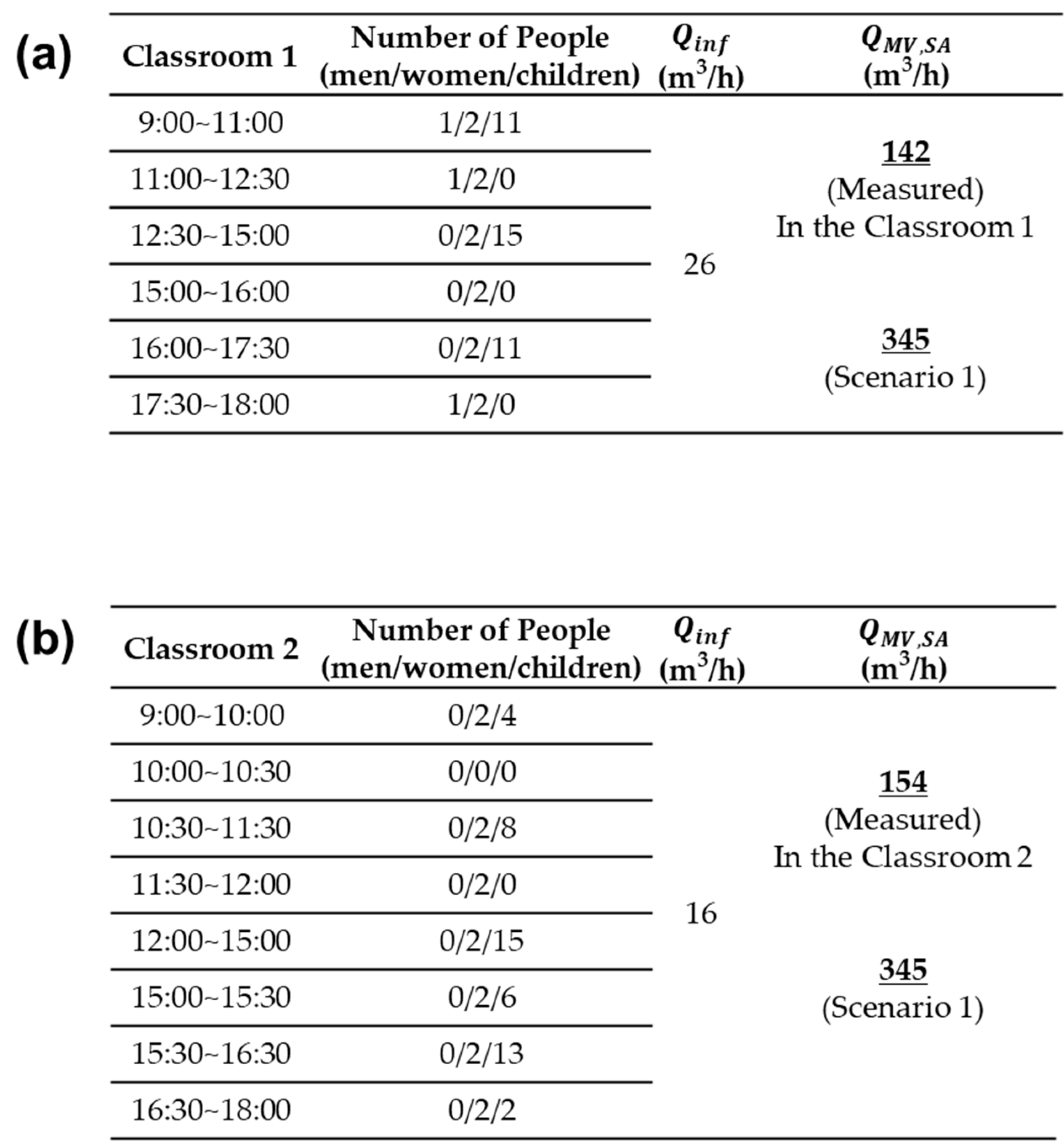
Figure 9 shows the days during the measurement period when the CO2 concentrations were the highest. Furthermore, the measurements on those specific days were compared with the calculated using Equations (2) and (7) and applied to derive the values, which were denoted as “Scenario1.” As the conditions of Scenario 1, is 345 m3/h that is the highest flowrate in Figure 8, is 0.35 and is 210 m3/h. Table 2 shows the values applied to the numerical model over time for Scenario 1. Figure 9a shows the results of the measurements in Classroom 1. For the measured concentration in Classroom 1, the CO2 concentration was almost over 1000 ppm. When the scenario 1 was applied, CO2 concentrations were maintained below 1000 ppm during class time. Figure 9b shows the CO2 concentrations measured on the same day for Classroom 2. Scenario 1, as calculated in Figure 9a, also allowed us to maintain CO2 concentrations below 1000 ppm.
4.2. Decreasing the concentration of PM2.5
Figure 10 shows the measured data of indoor PM2.5 concentration and the simulation under the conditions of scenarios 1, 2, and 3 on the day with the highest indoor PM2.5 concentration. As the conditions of scenario 2, is 345 m3/h, is 0.35 and is 480 m3/h that is a 4 level flowrate of air purifier. As the conditions of scenario 3, is 345 m3/h, is 0.75 which has a MERV 13 filter grade and of 210 m3/h.
An average PM2.5 concentrations of a day under Scenario 1 (=345 m3/h) was about 20% higher than the measured PM2.5 concentration (=157 m3/h). This indicated that increasing leads to an influx of outdoor PM2.5. To mitigate the increase in indoor PM2.5 concentrations, it is necessary to either increase the CADR () of air purifiers or improve the filtration efficiency of the mechanical ventilation system filters. An average PM2.5 concentrations under Scenario 2 where of an air purifier is increased from 210 m3/h to 480 m3/h was only about 16% lower than the measured PM2.5 concentration (=210 m3/h).
In Scenario 3, the filter in a ventilation system was replaced to a MERV13 filter and flowrate of mechanical ventilation was increased to 345 m3/h. The PM2.5 concentration (, = 345 m3/h) obtained from Scenario 3 was 52% lower than the measured PM2.5 concentration (, = 157 m3/h). Even the day which had significantly high indoor PM2.5 concentration (average PM2.5 concentration = 26.5 μg/m³), the average daily PM2.5 concentration can be reduced to below 15 μg/m³ under Scenario 3. The indoor PM2.5 concentration was effectively reduced by enhancing the collection efficiency of the mechanical ventilation filter when the mechanical ventilation flow rate was enough high.
5. Conclusions
This study presents an approach for reducing indoor PM2.5 concentrations while ensuring that the ventilation flow rate maintains indoor CO2 concentrations below 1000 ppm. The approach utilizes a numerical analysis model consistent with the measured indoor CO2 and PM2.5 concentrations in kindergartens. Scenarios involving the operation of mechanical ventilation systems and air purifiers for indoor air quality management were presented.
The mechanical ventilation rate necessary to maintain a CO2 concentration below 1000 ppm was calculated. It can be deduced that approximately 20.4 m3/h of ventilation per child is required for kindergarten classrooms. These results can be useful in designing a mechanical ventilation system for rooms in a kindergarten.
If a high collection efficiency of filter is equipped in mechanical ventilation system, that an increased flowrate of mechanical ventilation lead to the result that show a greater reduction in indoor PM2.5. Consequently, a mechanical ventilation filter with a high collection efficiency for PM2.5 is advisable, especially in multi-use facilities such as kindergartens, where a significant amount of CO2 is generated via respiration.
Funding
This research was supported by a grant from the Basic Research Program funded by the Korea Institute of Machinery and Materials (grant number NK243A).
References
- Jones, A.P. Indoor air quality and health. Atmos Environ 1999, 33, 4535–4564. [CrossRef]
- Robinson, J.; Nelson, W.C. National Human Activity Pattern Survey Data Base; USEPA: Research Triangle Park, 1995; p. NC2.
- WH Organization. Air quality guidelines global update 2021: Particulate matter (PM2.5 and PM10), Ozone, Nitrogen Dioxide, Sulfur Dioxide and Carbon Monoxide.
- Talbott, E.O.; Arena, V.C.; Rager, J.R.; Clougherty, J.E.; Michanowicz, D.R.; Sharma, R.K.; Stacy, S.L. Fine particulate matter and the risk of autism spectrum disorder. Environ Res 2015, 140, 414–420. [CrossRef]
- Zeng, X.; Liu, D.; Wu, W. PM2.5 exposure and pediatric health in e-waste dismantling areas. Environ Toxicol Pharmacol 2022, 89, 103774. [Google Scholar] [CrossRef] [PubMed]
- de Oliveira, B.F.A.; Ignotti, E.; Artaxo, P.; do Nascimento Saldiva, P.H.; Junger, W.L.; Hacon, S. Risk assessment of PM2.5 to child residents in Brazilian Amazon region with biofuel production. Environ Health 2012, 11. [Google Scholar] [CrossRef] [PubMed]
- Bogdanovica, S.; Zemitis, J.; Bogdanovics, R. The effect of CO2 concentration on children’s well-being during the process of learning. Energies 2020, 13. [Google Scholar] [CrossRef]
- Guidelines for Indoor Air Quality Management in Preschools; Ministry of the Environment, 2021.
- Park, S.; Lee, J.; Yang, Y.; Lee, S.; Park, J.. (2017). A Survey of the Indoor Air Quality in the Child Care Center. . Korean Soc. Living Environ 2017, 24, No. 6, 733~743. [CrossRef]
- Phee, Y. G.; Jung, J. H.; Nam, M. R. Exposure assessment of PM2. 5 in manufacturing industry office building. J Korean Soc Occup Environ Hyg 2013, 23.4: 356-366.
- Han, B.; Hong, K.; Shin, D.; Kim, H.J.; Kim, Y.J.; Kim, S.B.; Kim, S.; Hwang, C.H.; Noh, K.C. Field tests of indoor air cleaners for removal of PM2.5 and PM10 in elementary school classrooms in Seoul, Korea. Aerosol Air Qual Res 2022, 22, 210383. [Google Scholar] [CrossRef]
- Pacitto, A.; Amato, F.; Moreno, T.; Pandolfi, M.; Fonseca, A.; Mazaheri, M.; Stabile, L.; Buonanno, G.; Querol, X. Effect of ventilation strategies and air purifiers on the children’s exposure to airborne particles and gaseous pollutants in school gyms. Sci Total Environ 2020, 712, 135673. [Google Scholar] [CrossRef]
- Noh, K.-C.; Yook, S.-J. Evaluation of clean air delivery rates and operating cost effectiveness for room air cleaner and ventilation system in a small lecture room. Energy Build 2016, 119, 111–118. [Google Scholar] [CrossRef]
- Lee, M. An analysis on the concentration characteristics of PM2.5 in Seoul, Korea from 2005 to 2012. Asia-Pacific J Atmos Sci 50 (Suppl 1), pp 585–594 (2014). [CrossRef]
- Martins, Nuno R., and Guilherme Carrilho da Graça. “Impact of outdoor PM2. 5 on natural ventilation usability in California’s nondomestic buildings.” Applied energy 189 (2017): 711-724. [CrossRef]
- Cho, Y.; Lee, J.-Y.; Kwon, S.-B.; Park, D.-S.; Park, J.-H.; Cho, K.-C. The distribution characteristics of carbon dioxide in indoor school spaces. J Korean Soc Atmos Environ 2011, 27, 117–125. [CrossRef]
- Noh, K.-C.; Oh, M.-D. Variation of clean air delivery rate and effective air cleaning ratio of room air cleaning devices. Build Environ 2015, 84, 44–49. [Google Scholar] [CrossRef]
- Shaughnessy, R.J.; Sextro, R.G. What is an effective portable air cleaning device? A review. J Occup Environ Hyg 2006, 3, 169–81. [Google Scholar] [CrossRef]
- Shin, D.; Kim, Y.; Hong, K.; Lee, G.; Park, I.; Han, B. The actual efficacy of an air purifier at different outdoor PM2.5 concentrations in residential houses with different airtightness. Toxics 2022, 10, 616. [Google Scholar] [CrossRef] [PubMed]
- Cho, J.; Yoo, C,; Kim, Y. Effective Opening Area and Installation Location of Windows for Single Sided Natural Ventilation in High-rise Residences. Journal of Asian Architecture and Building Engineering 2012, 11:2, 391-398. [CrossRef]
- Malik, N. Field studies of dependence of air infiltration on outside temperature and wind. Energy Build 1978, 1, 281–292. [CrossRef]
- Franco, A.; Schito, E. Definition of optimal ventilation rates for balancing comfort and energy use in indoor spaces using CO2 concentration data. Buildings 2020, 10, 135. [CrossRef]
- Korea Meteorological Administration. Report of Global Atmosphere Watch; Vol. 61, 2021.
Figure 1.
Schematic of experimental setup: A floor plan view of arrangement.
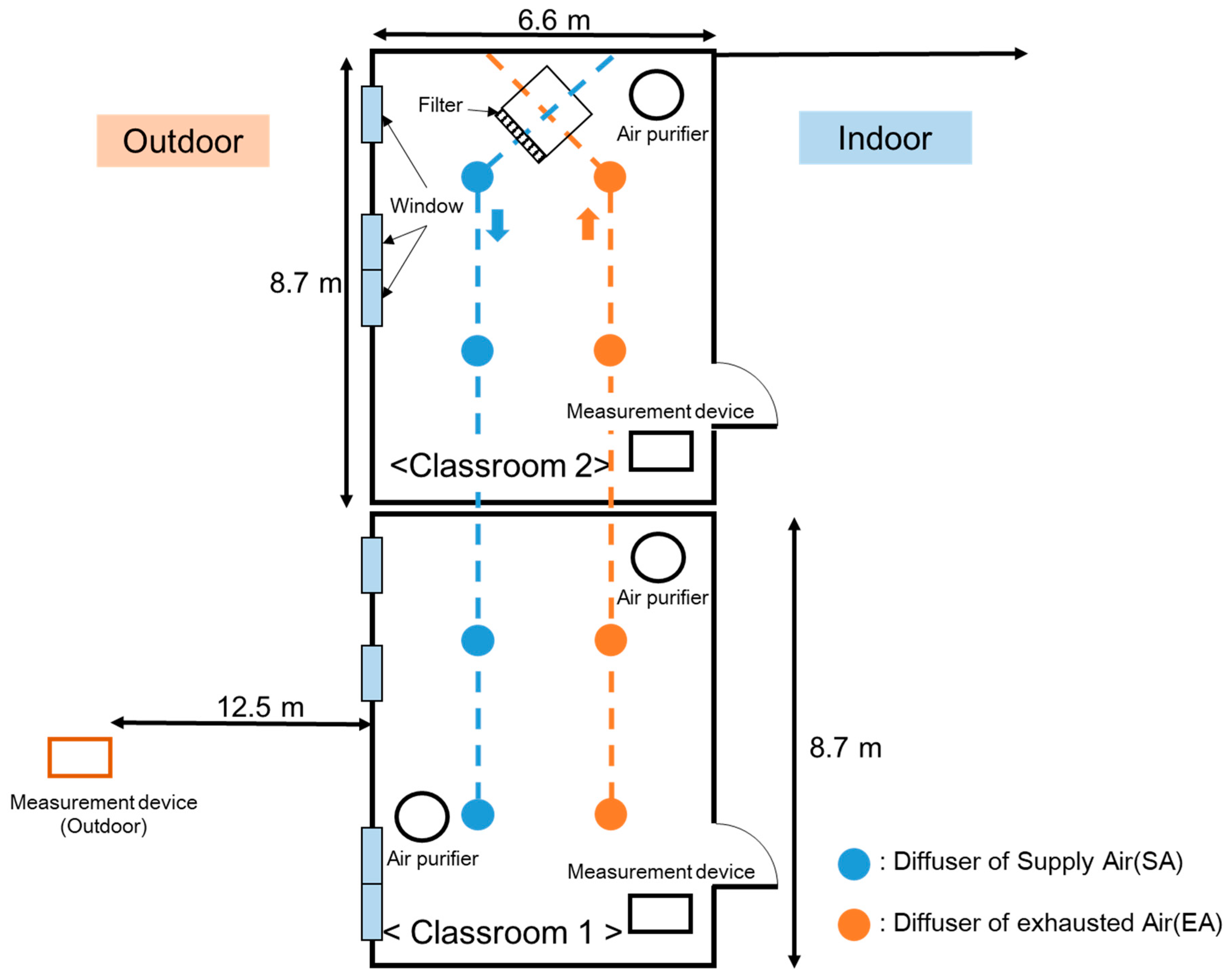
Figure 2.
Diagrams of (a) CO2 model and (b) PM2.5 model of indoor.
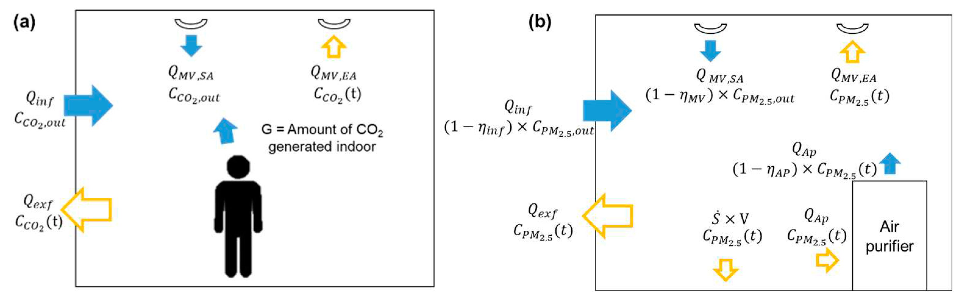
Figure 3.
Measuring natural ventilation flowrate of indoor when all of windows is (a) closed and (b) opened. [Classroom 1, Classroom 2].
Figure 3.
Measuring natural ventilation flowrate of indoor when all of windows is (a) closed and (b) opened. [Classroom 1, Classroom 2].
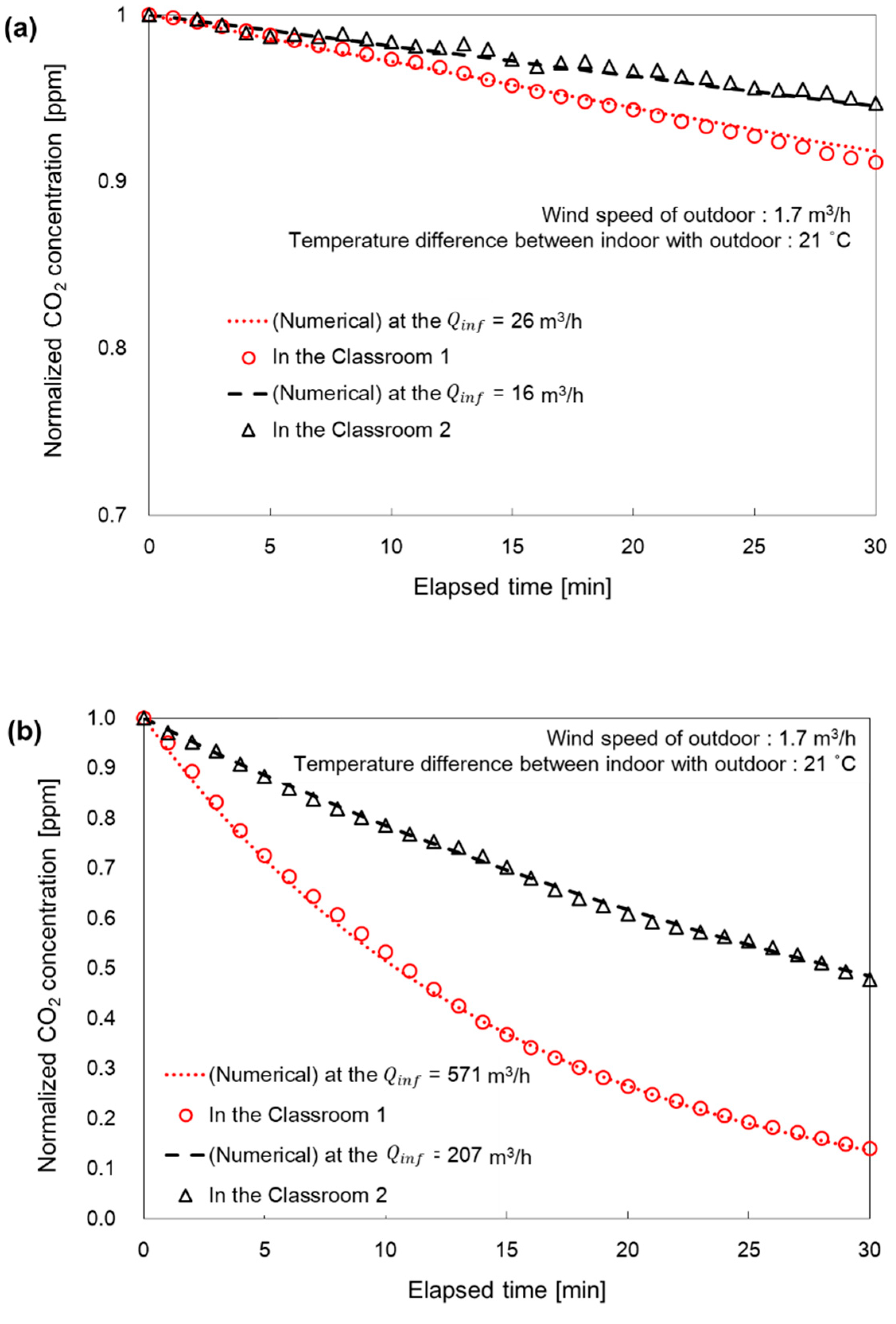
Figure 4.
Saturated PM2.5 concentration of indoor when outdoor condition is stable according to time.
Figure 4.
Saturated PM2.5 concentration of indoor when outdoor condition is stable according to time.
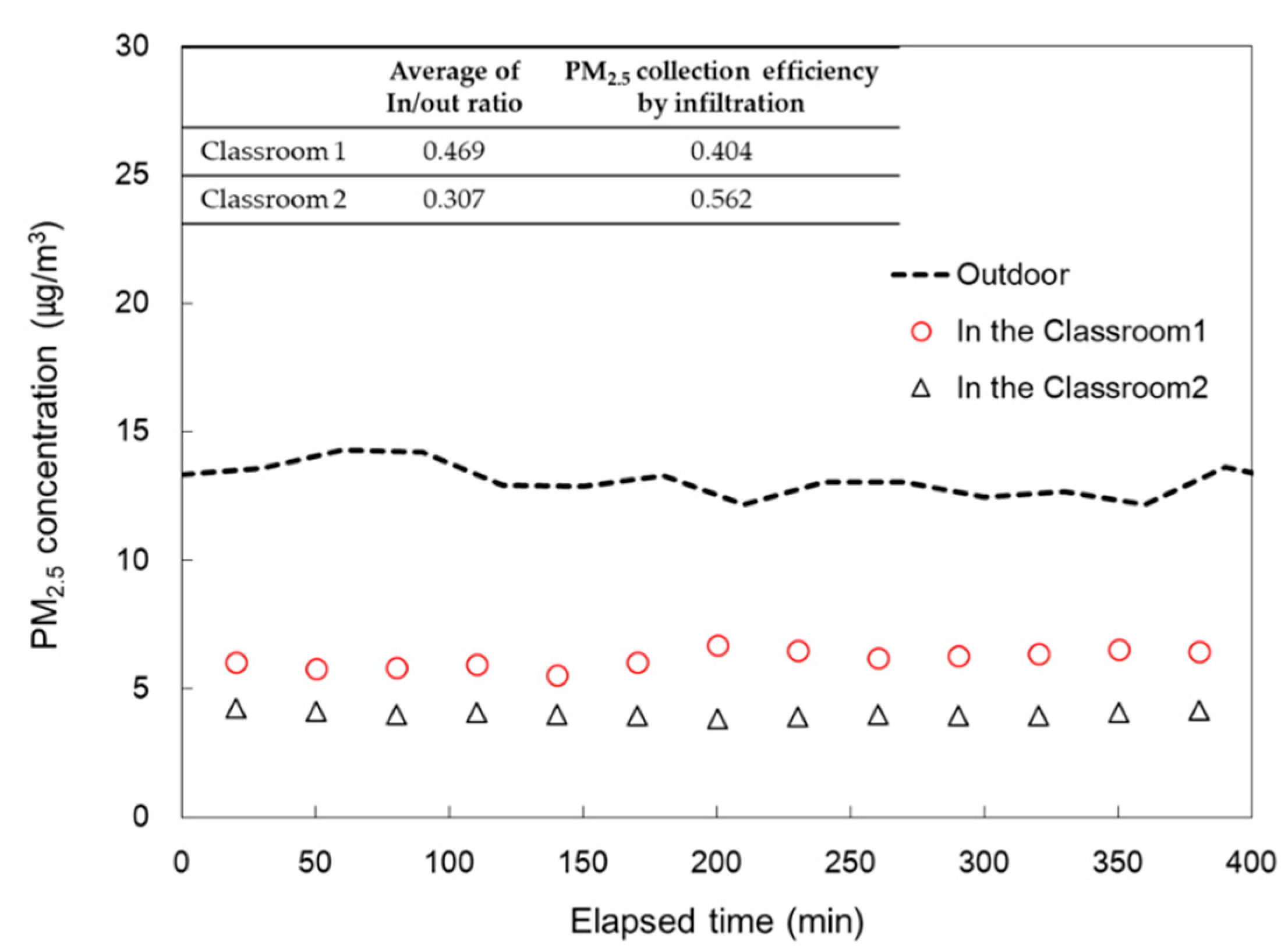
Figure 5.
Measuring the EACR of air purifiers in Classroom 1 and Classroom 2.
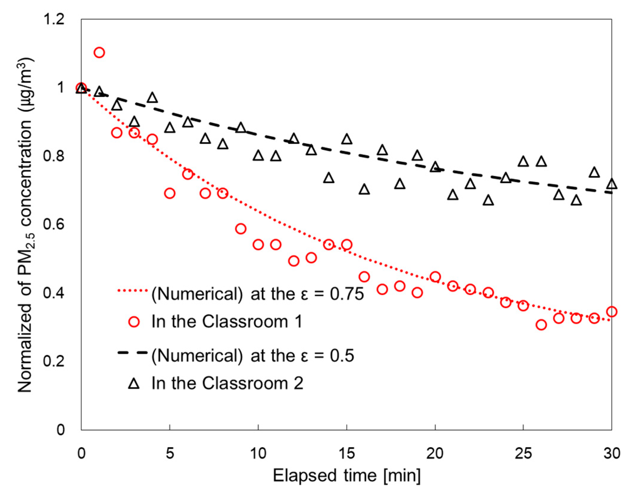
Figure 6.
Comparison CO2 concentration that obtained by numerical model in (a) Classroom 1 at 23. 01. 03, (b) Classroom 2 at 23. 01. 03, (c) Classroom 1 at 23. 01. 11, (d) Classroom 2 at 23. 01. 11 with measured data of CO2 concentration.
Figure 6.
Comparison CO2 concentration that obtained by numerical model in (a) Classroom 1 at 23. 01. 03, (b) Classroom 2 at 23. 01. 03, (c) Classroom 1 at 23. 01. 11, (d) Classroom 2 at 23. 01. 11 with measured data of CO2 concentration.
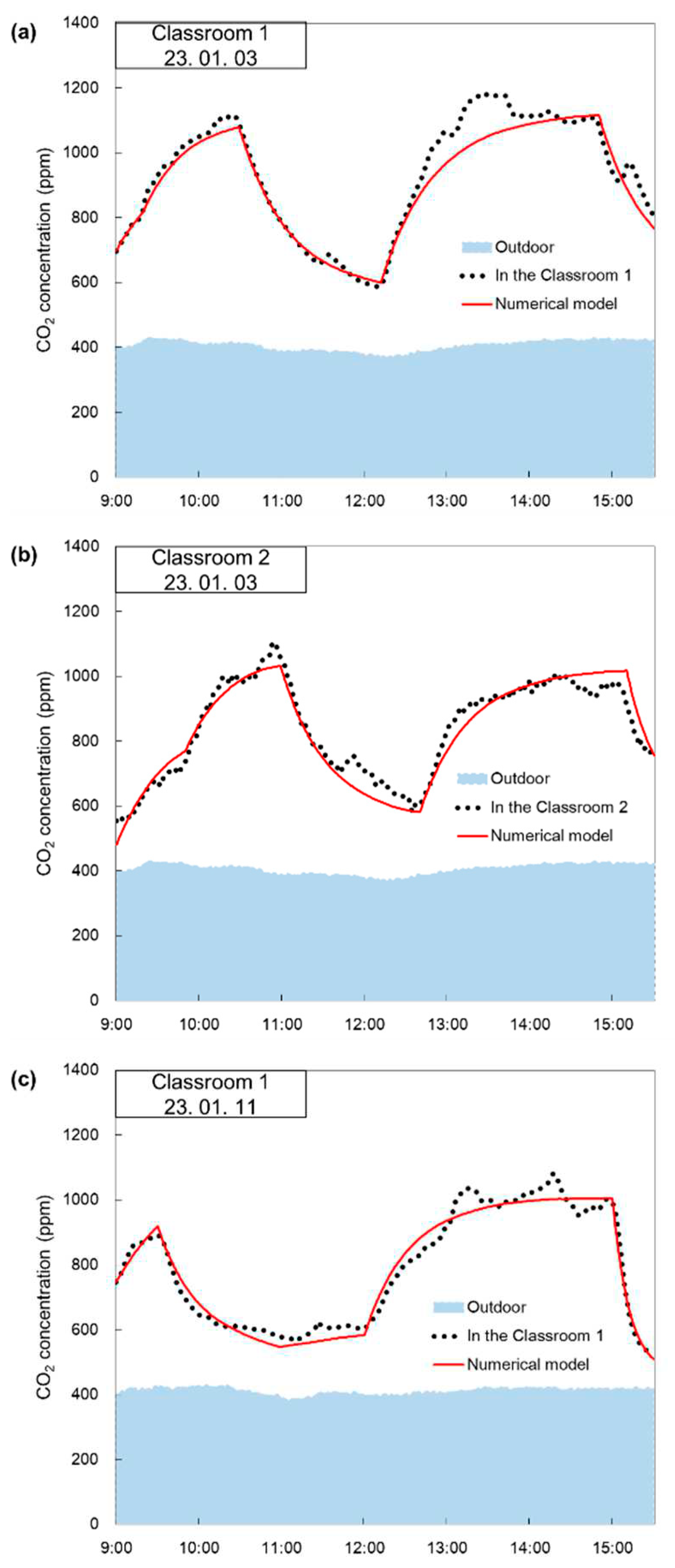
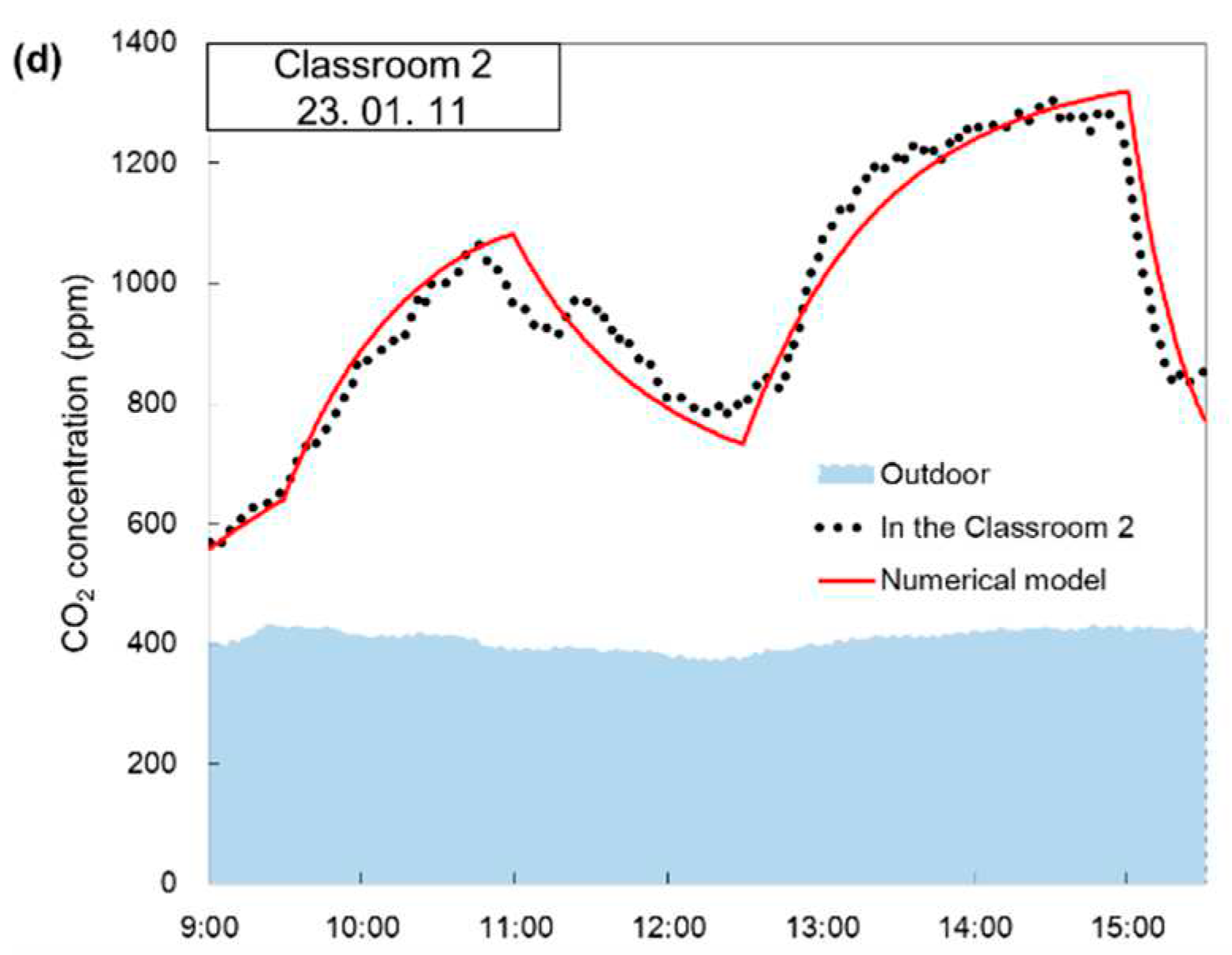
Figure 7.
Comparison with measured data of PM2.5 concentration that obtained by numerical model in (a) Classroom 1 at 23. 01. 03, (b) Classroom 2 at 23. 01. 03, (c) Classroom 1 at 23. 01. 11, (d) Classroom 2 at 23. 01. 11 with measured data of PM2.5 concentration.
Figure 7.
Comparison with measured data of PM2.5 concentration that obtained by numerical model in (a) Classroom 1 at 23. 01. 03, (b) Classroom 2 at 23. 01. 03, (c) Classroom 1 at 23. 01. 11, (d) Classroom 2 at 23. 01. 11 with measured data of PM2.5 concentration.
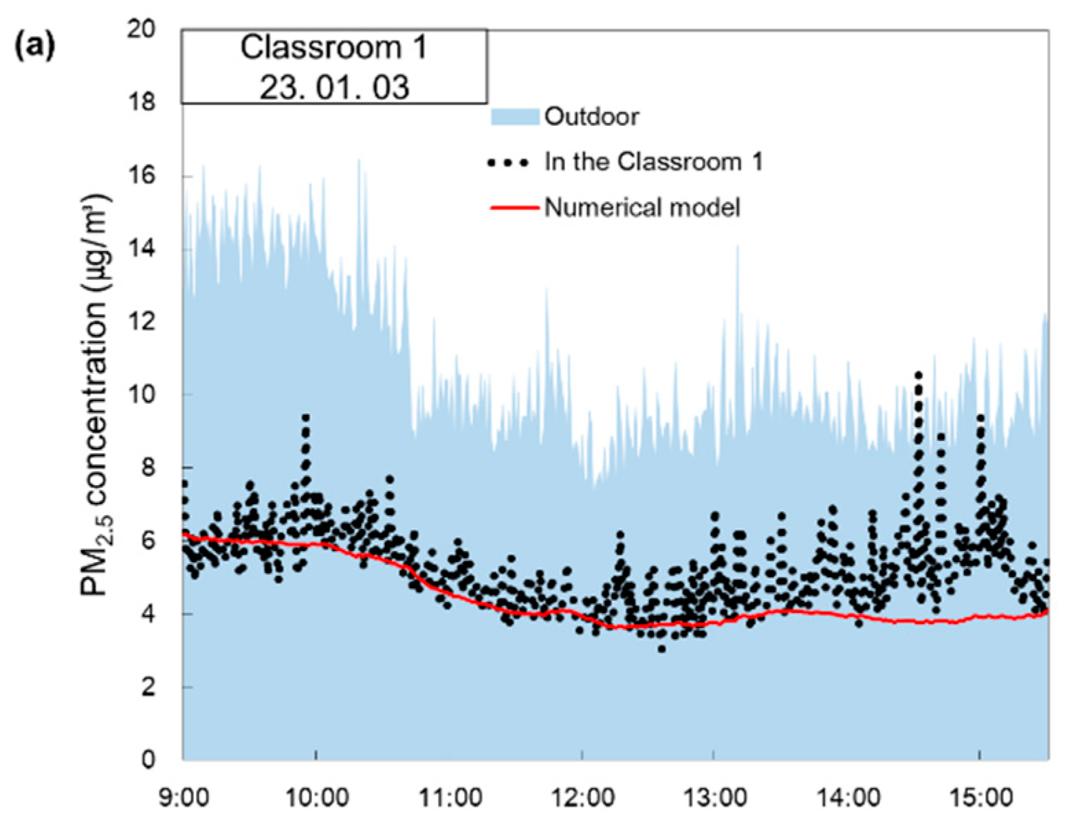
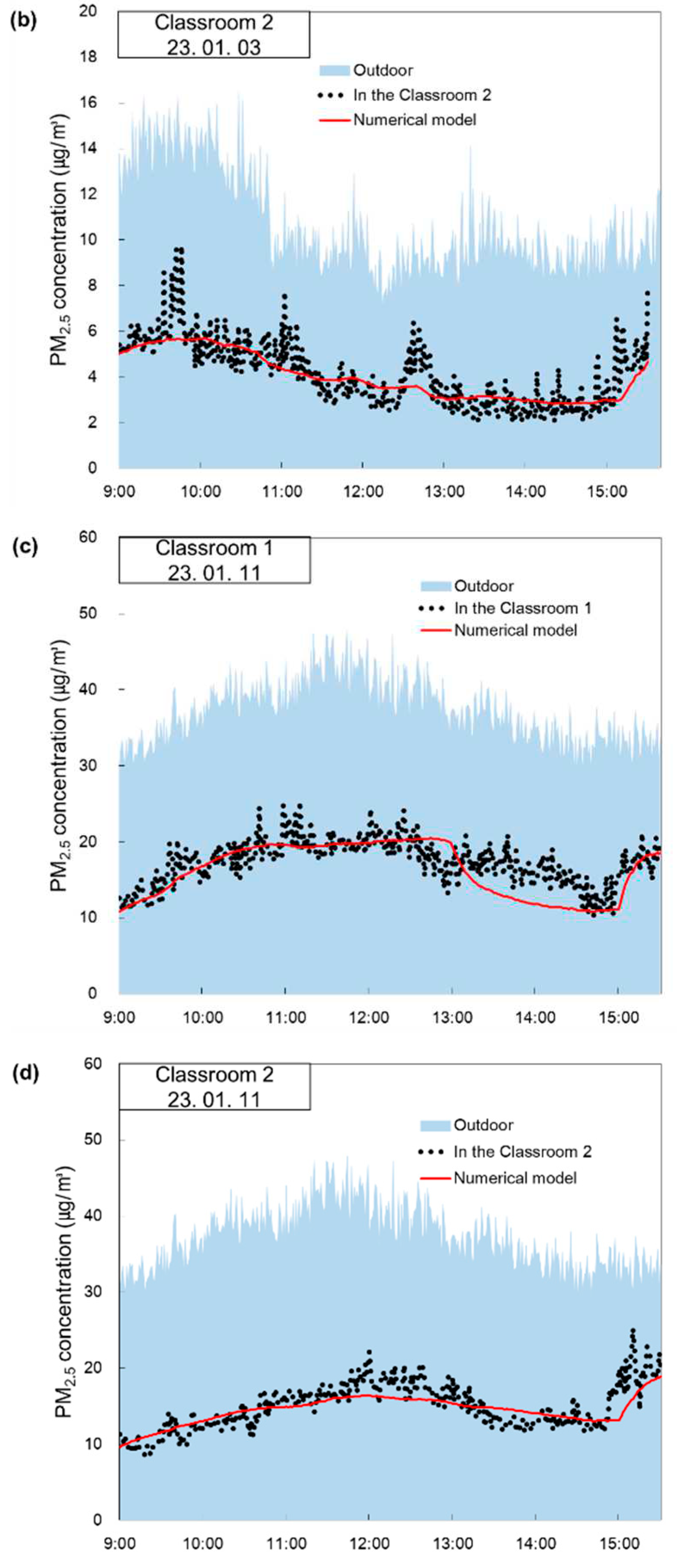
Figure 8.
Flowrate of mechanical ventilation required, according to the number of children occupied indoor.
Figure 8.
Flowrate of mechanical ventilation required, according to the number of children occupied indoor.
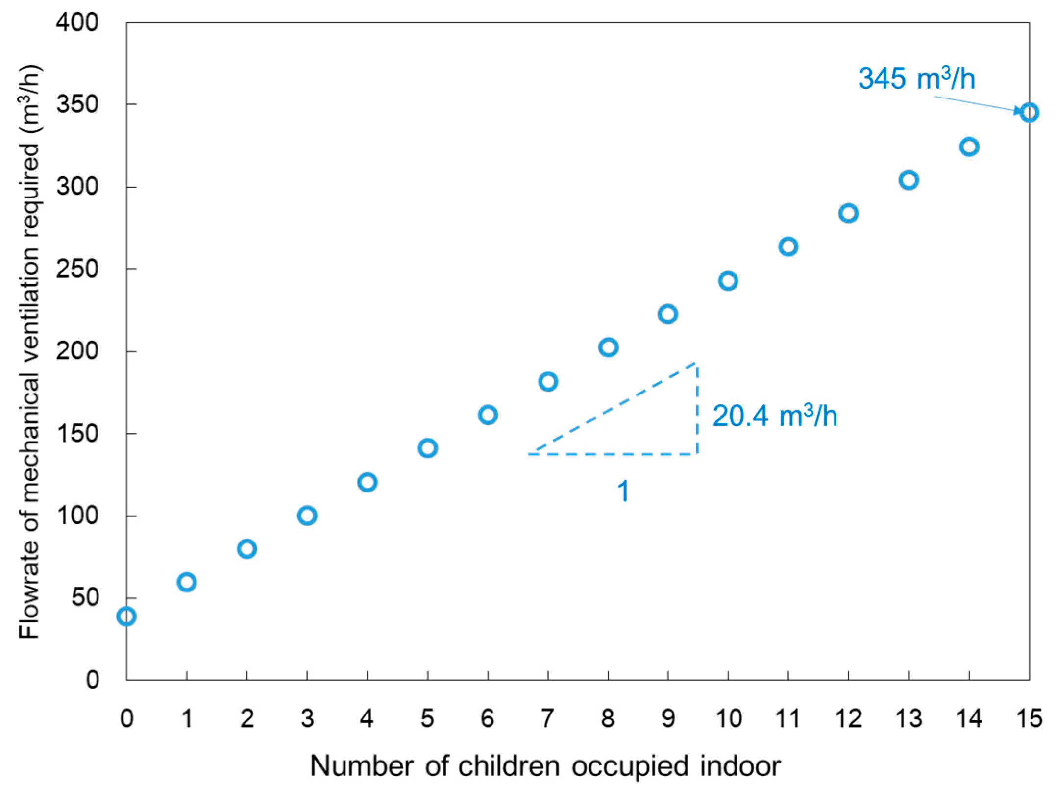
Figure 9.
Graph showing that indoor CO2 concentration maintain below 1000 ppm in ‘Scenario 1′ that the ideal amount of ventilation is applied in a day when indoor CO2 concentration was highest from January to March 2023 at (a) Classroom 1, (b) Classroom 2.
Figure 9.
Graph showing that indoor CO2 concentration maintain below 1000 ppm in ‘Scenario 1′ that the ideal amount of ventilation is applied in a day when indoor CO2 concentration was highest from January to March 2023 at (a) Classroom 1, (b) Classroom 2.
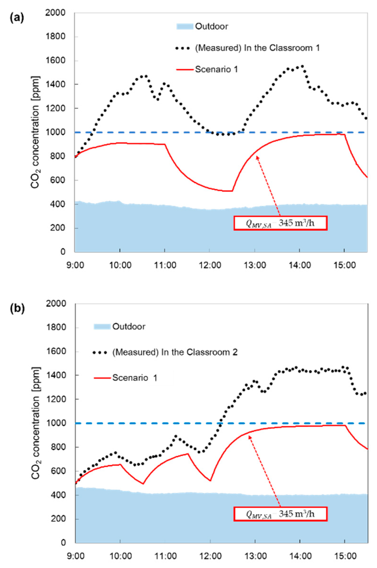
Figure 10.
Graph of comparing PM2.5 concentration over time that obtained from simulation under conditions of Scenarios with measured data to show an effect of decreasing PM2.5 concentration.
Figure 10.
Graph of comparing PM2.5 concentration over time that obtained from simulation under conditions of Scenarios with measured data to show an effect of decreasing PM2.5 concentration.


Table 1.
Indoor Condition about CO2 and PM2.5 concentration according to time for Comparison in (a) Classroom 1 at 23. 01. 03, (b) Classroom 2 at 23. 01. 03, (c) Classroom 1 at 23. 01. 11, (d) Classroom 2 at 23. 01. 11.
Table 1.
Indoor Condition about CO2 and PM2.5 concentration according to time for Comparison in (a) Classroom 1 at 23. 01. 03, (b) Classroom 2 at 23. 01. 03, (c) Classroom 1 at 23. 01. 11, (d) Classroom 2 at 23. 01. 11.
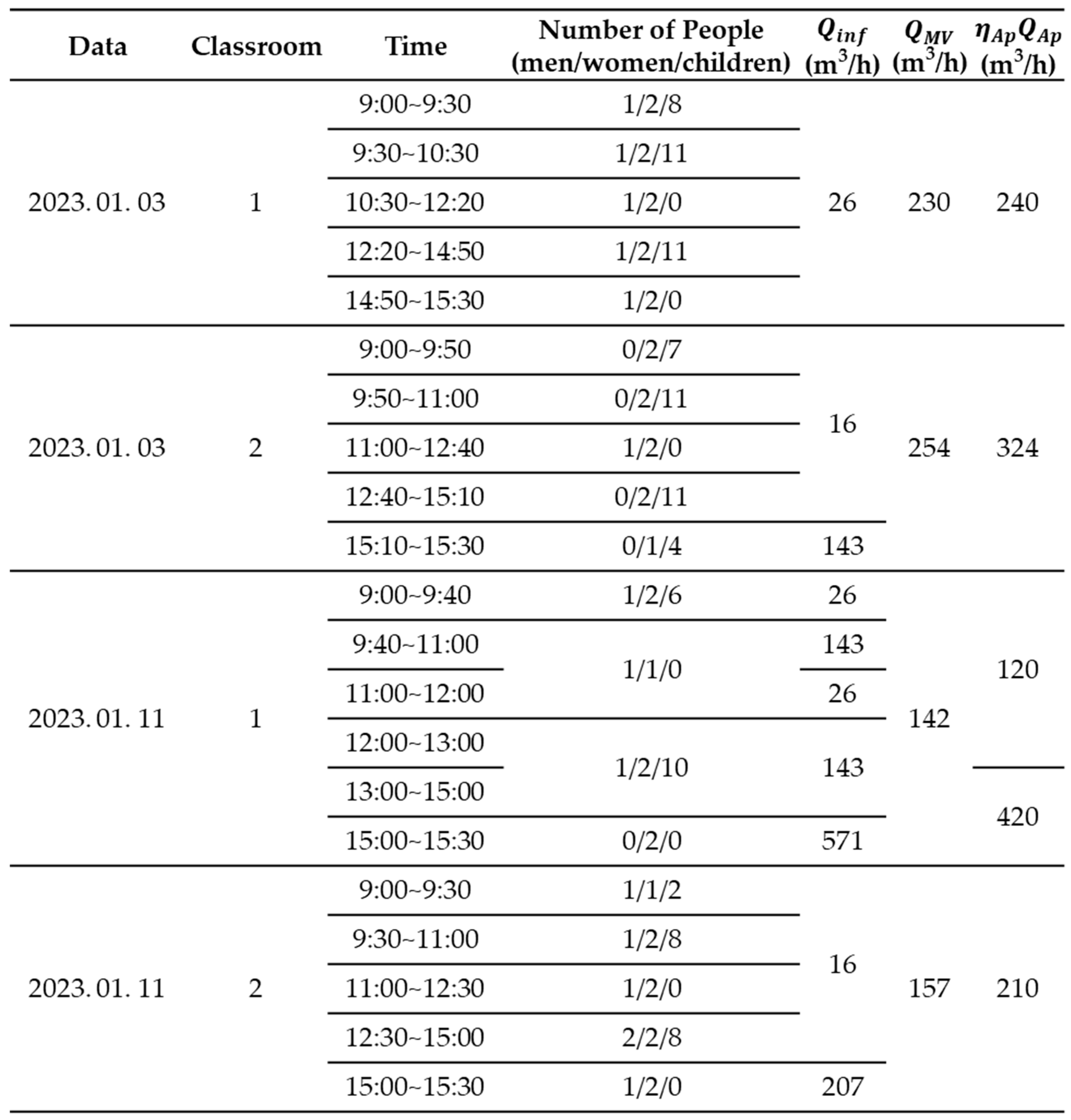
Table 2.
The indoor condition of the Numerical Model about CO2 in a day when CO2 concentration was highest from January to March 2023 at (a) Classroom 1, (b) Classroom 2.
Table 2.
The indoor condition of the Numerical Model about CO2 in a day when CO2 concentration was highest from January to March 2023 at (a) Classroom 1, (b) Classroom 2.
Disclaimer/Publisher’s Note: The statements, opinions and data contained in all publications are solely those of the individual author(s) and contributor(s) and not of MDPI and/or the editor(s). MDPI and/or the editor(s) disclaim responsibility for any injury to people or property resulting from any ideas, methods, instructions or products referred to in the content. |
© 2023 by the authors. Licensee MDPI, Basel, Switzerland. This article is an open access article distributed under the terms and conditions of the Creative Commons Attribution (CC BY) license (http://creativecommons.org/licenses/by/4.0/).
Copyright: This open access article is published under a Creative Commons CC BY 4.0 license, which permit the free download, distribution, and reuse, provided that the author and preprint are cited in any reuse.


