Submitted:
11 September 2023
Posted:
13 September 2023
You are already at the latest version
Abstract
In view of the problem that the hot and cold loads of mushroom houses are affected by multiple factors such as environment, mushrooms, and equipment, which are difficult to accurately model, this paper proposes a short-term load prediction method based on empirical wavelet transform (EWT) and mixed autoregressive integrated moving average (ARIMA) and convolutional bi-directional short- and long-term attention mechanism (CNN-BiLSTM-Attention). The method first uses the Boruta algorithm to filter the input characteristics, and then uses the EWT method to decompose the mushroom house load data into 4 modal components. Then the Lempel-Ziv method is introduced to divide the modal components into two categories of high and low frequencies, and the CNN-BiLSTM-Attention and ARIMA prediction models are constructed separately. Finally, the two types of prediction results are superimposed and reconstructed to obtain the final load prediction value. The test results show that the Boruta algorithm can effectively filter out the characteristics of key influencing factors. Compared with the Spearman and Pearson correlation coefficient methods, the mean absolute error (MAE) of the prediction results is reduced by 14.72% and 3.75%, respectively; compared with the ensemble empirical mode decomposition (EEMD) method, the EWT method can increase the decomposition and reconstruction error by 103 orders of magnitude, which can effectively improve the prediction accuracy of the model; compared with the individual neural network model, the prediction effect of the model proposed in this paper has obvious advantages, and the MAE, root mean square error (RMSE) and mean absolute percentage error (MAPE) of the prediction results are reduced respectively. 31.06%, 26.52% and 39.27%.
Keywords:
Factory mushroom house
; Empirical wavelet transform
; Lempel-Ziv algorithm
; Boruta algorithm
orders of magnitude, which can effectively improve the prediction accuracy of the model; compared with the individual neural network model, the prediction effect of the model proposed in this paper has obvious advantages, and the MAE, root mean square error (RMSE) and mean absolute percentage error (MAPE) of the prediction results are reduced respectively. 31.06%, 26.52% and 39.27%.
1. Introduction
In recent years, the proportion of domestic edible fungus factory production models in the edible fungus industry has been continuously increasing [1].According to statistics, energy accounts for 20% to 30% of the total cost of factory production of edible mushrooms [2], of which the air-conditioning system used to regulate the temperature of the mushroom house accounts for about 40% of the total cost of energy [3].Saving air-conditioning energy consumption has become an urgent problem for edible fungus factories.
The prediction of the hot and cold load of the mushroom house is an important research content for the energy-saving operation of the air-conditioning system [4]. Due to the influence of climate, equipment working conditions, edible fungus growth status, etc., the traditional mechanism model is difficult to accurately model. With the technological development of the Internet of Things, the cost of obtaining a large amount of real-time data has been reduced. In this context, the data-driven prediction method represented by deep neural networks has attracted widespread attention from scholars at home and abroad [5-13]. Long short-term memory (LSTM) is widely used in the field of load prediction because of its unique gating mechanism [14-18]. Zhou et al. [19] used LSTM and back propagation neural network (BPNN) to predict the power consumption of air conditioners. The results show that compared with BPNN, the mean absolute percentage error (MAPE) of LSTM's predicted daily power consumption is reduced by 49%, and the MAPE of power consumption is reduced by 36.61%. Bi-directional long short-term memory (BiLSTM) is an improved network of LSTM, which can extract sequence information from both front and back directions at the same time, and can better capture bidirectional timing characteristics [20]. In order to further explore the spatial characteristics of influencing factors, Kim et al. [21] proposed a hybrid model short-term load prediction method based on convolutional neural network (CNN) and LSTM, which constructs a continuous feature sequence based on historical load, meteorological information, and date information in a sliding window of time, uses the CNN layer to extract spatial features, and then uses the LSTM network to complete the short-term load prediction. The results show that compared with using LSTM alone, its MAPE is reduced by 53.36%. Attention mechanism is a resource allocation mechanism that simulates the attention of the human brain. It is widely used in the field of time series prediction because it can enhance the weight of key influencing factors. Zhang et al. [22] used the temporary convolutional network (TCN) method combined with attention to predict wind power. Compared with the prediction model that did not introduce attention, the root mean square error (RMSE) was reduced by 16.46%.
The above-mentioned hybrid prediction model does not mine the characteristics of the original data of the load, and simply pursues high-precision prediction based on different algorithm performance. In order to select a suitable prediction method for the characteristics of the target data, Gao et al. [23] used empirical mode decomposition (EMD) to decompose the power load data. However, modal aliasing and endpoint effects will occur when the EMD method is decomposed. To this end, Li et al. [24] used the ensemble empirical mode decomposition (EEMD) method to decompose the load data into multiple eigenmode functions, and construct BPNN separately for prediction based on the characteristics of different frequency signals after decomposition. Although the EEMD method can reduce errors due to modal aliasing and endpoint effects, adding white noise multiple times will lead to increased computational complexity. Empirical wavelet transform (EWT) method was proposed by Gilles in 2013. It can adaptively select frequency bands, overcome modal aliasing, reduce computational complexity, and has good application prospects [25].
In summary, this paper proposes a method for predicting the hot and cold load of factory mushroom house based on EWT decomposition in view of the rapid prediction of the hot and cold load of short-term mushroom house. The method first uses the EWT method to decompose the mushroom house load into multiple eigenmode functions, and then uses the Lempel-Ziv algorithm to classify the modal components, and then reconstructs the components into high-frequency and low-frequency parts, and then uses the CNN-BiLSTM-Attention model and the autoregressive integrated moving average (ARIMA) model for prediction. Finally, the measured data of an edible fungus factory is used for verification and analysis, and it is compared with the commonly used prediction methods to verify that the load prediction method proposed in this paper has a good prediction effect.
2. Materials and methods
2.1. Data source
The test site was located in a seafood mushroom company in Tongzhou District, Beijing. The length, width and height of the test mushroom house ware 14m, 8m and 5m. The ground of the mushroom house was hardened concrete, and the surrounding and roof enclosures of the mushroom house ware polyurethane sandwich color steel plates with a thickness of about 100mm.The mushroom house was equipped with fixed-frequency air conditioners, fresh air fans, exhaust fans, humidifiers and other control equipment.
In order to obtain relevant data affecting the load of the mushroom house, the air temperature and humidity inside and outside the mushroom house were continuously measured using HOBO U23-001A (accuracy: ±0.2℃, ±2.5%), The working status of the air conditioner is checked and monitored by HOBO CTV-C(accuracy: ±5A) current collector, and the sampling interval were set to 1 minute. The fresh air wind speed is measured using Delta HD2903T wind speed sensor (accuracy: ±3%); the CO2 concentration was measured using Vaisala's GMP252 sensor; the solar radiation was measured using Kipp&Zonen's SMP3 sensor; the wall heat flux was measured using Hukseflux HFP01 heat flux sensor, which were connected to Campbell's CR1000X data collector for continuous recording, and the sampling interval was 1 minute.
The deployment of mushroom house measuring equipment is shown in Figure 1. The temperature and humidity sensor was evenly arranged in the middle of the mushroom house with 5 measurement points in the east-west direction, and two layers are arranged at equal distances in the vertical direction of the cultivation shelf, with a total of 10 sensors; the wind speed sensor was installed at the air inlet of the fresh air pipeline; the CO2 sensor was arranged in the center of the house; the outdoor air temperature, humidity and solar radiation sensor were installed through a pole at a distance of 5m from the mushroom house, with a height of 2m.Collected data from July 11, 2022 to September 15, 2022, totaling 729,300 pieces.
2.2. Data processing
Data preprocessing includes three parts: outlier handling, feature filtering, and normalization, as shown in
Figure 2
.
The acquired data is missing and abnormal due to the equipment itself or transmission, which affects the accuracy of the prediction model. For missing data, the front and rear data of the missing position are used to fill the gaps by linear interpolation, and the calculation method is shown in equation (1); for abnormal data, the mean method is used for smoothing and filtering, and the calculation method is shown in equation
(2).
Where is the missing data at time ; is the original data at time ; is the original data at time .
Where
is abnormal data,
,
are adjacent to the valid data.
In order to improve the efficiency of model prediction, the Boruta algorithm is used to filter out key input features and construct a feature set for model training. The Boruta algorithm calculates the binomial distribution of feature selection probability through multiple iterations, as shown in Figure 3.
The red part is the rejection area, and the features that fall into this area are removed during the iteration process; the blue part is the uncertain area, and the features that fall into this area are in a pending state during multiple iterations, and need to be further determined according to the screening threshold and the importance of the features; the green part is the acceptance area, and the features that fall into this area are directly retained.
In order to eliminate the influence of the load parameters of the mushroom house on the training of the neural network prediction model due to the difference between the dimensions, each factor needs to be normalized, and the calculation method is shown in equation (3).
Where
is the
maximum value,
is the minimum value, and
is the normalized value.
2.3. Model experimental environment
The computer configuration of the experimental platform is as follows: equipped with AMD Ryzen (TM) 7 5800H CPU, NVIDIA GeForce GTX 1650 4G GPU, 16GB of memory, and 64-bit Windows 10 operating system. The software uses Keras as a deep learning tool, Tensorflow-gpu-2.3 as a deep learning framework, the programming language is Python, the Python version is 3.7, and the integrated development environment is Visual Studio Code.
2.4. Model prediction evaluation indicators
In order to quantitatively evaluate the effect and accuracy of the model's prediction, this paper uses root mean square error (RMSE), mean absolute error (MAE), and (MAPE) as indicators to measure the prediction accuracy. The calculation methods of RMSE, MAE and MAPE are shown in equation (4), equation (5) and equation (6).
Where is the actual load, is the predicted load, and is the total number of data.
2.5. Process design
The model prediction process proposed in this article is shown in Figure 4, the specific steps are as follows:
1. Exception data processing. The interpolation method and smoothing filter method are used to process the missing and outlier values in the collected data, and a complete data set is obtained.
2. Load data decomposition. EWT method is used to decompose the load of the mushroom house into modal components of different scales, and the Lempel-Ziv method is used to classify the high and low frequencies of each modal component, and all components are reconstructed into high-frequency and low-frequency characteristic components.
3. Feature screening. Boruta algorithm is used to clarify the input characteristics of the neural network model, construct the input feature set, and divide the data set into training set, verification set, and test set in a 7:2:1 ratio.
4. Predictive model construction. For the high-frequency feature components, the data set in Step 3 is first normalized, and then the CNN-BiLSTM-Attention model is used to predict, and the high-frequency feature prediction results are obtained after inverse normalization; for the low-frequency feature components, an ARIMA prediction model is established to solve the defect that the neural network is insensitive to linear feature recognition, and then the results of the high and low frequency prediction model are superimposed and reconstructed to obtain the final result.
5. Model prediction. Based on the test data and model prediction values, the model error index is obtained to evaluate the model prediction performance.
2.6. Predictive model structure
The overall structure of the hybrid ARIMA and CNN-BiLSTM-Attention model proposed in this paper is shown in Figure 5.
Input layer: For the high-frequency component part of the load, the input features are filtered by the Boruta method to establish key feature vectors, and then the historical 4-hour load data is used to predict the load changes in the next 10 minutes, and the input features with a data dimension of [24,7] are constructed and input to the CNN layer; for the low-frequency component part of the load, it is directly entered into the ARIMA model.
CNN layer: Extract the input feature matrix information by setting the 2-layer CNN layer. After passing through the first layer, the data dimension becomes [24,7,15], through the pooling layer pooling, the data dimension is transformed into [24,3,15], and then input to the second layer convolution layer, the data dimension is transformed into [24,3,1], then add a single layer Squeeze layer, compress the data dimension to [24,3] and input to the BiLSTM layer. The above process activation functions all use the ReLU function.
BiLSTM layer: Set the BiLSTM layer to be a single layer, and the activation function is Tanh. After passing through the BiLSTM layer, the data dimension becomes [24,128].
Attention layer: Due to the different degree of influence of various influencing factors on the load in the time series, an attention mechanism is introduced, and the calculation process is shown in equation (7) and (8).
Where, K, V, Q-Key, Value, Query, the dimensions are all [24,128]; F(Q,K) the similarity between Query and Key is calculated by the dot product method of Query and Key.
ARIMA layer: The ADF unit root method is used to detect that the low-frequency load part is a non-stationary sequence. After a differential transformation, it is a stationary sequence and then input to the ARIMA layer. The p, d, and q are 2, 1, and 1 respectively.
Output layer: Add the Dropout layer before the output layer to inactivate the neurons (the inactivation rate is 0.1) to prevent overfitting of the high-frequency part. After inactivation, the data dimension is [32], and then connect the output result of the 1-layer fully connected layer, and the low-frequency load prediction result obtained from the output of the ARIAM layer is reconstructed to obtain the final load prediction value.
3. Results
3.1. Analysis of feature set construction method
The original data has a total of 9 input characteristics, which can be divided into three categories: outdoor climatic factors, indoor environmental factors, and equipment working status, as shown in Table 1.
The Boruta algorithm is used to filter the above characteristic factors, and the total number of iterations of the Boruta algorithm is set to 80. The iteration process is shown in Table 2. Screening was carried out through the Boruta algorithm, and the algorithm stopped when it was iterated to 38 times. Among them, 2 input features were rejected and 7 input features were accepted, including outdoor temperature, outdoor humidity, heat flux, indoor temperature, indoor CO2 concentration, fresh air volume and air conditioning opening time.
In order to verify the performance of the Boruta method in feature selection, the performance of the Boruta method, the Person correlation coefficient method and the Spearman correlation coefficient method were verified through the constructed prediction model, and the original data was used as a comparison. The results are shown in Table 3.
It can be seen from Table 3 that after screening by the Boruta method, the model has the best prediction effect. Its MAE is 0.591kW, which is lower than the control group, Spearman correlation coefficient method, and Pearson correlation coefficient method, respectively 16.88%、14.72%、3.75%; Its RMSE is 1.056kW, which is lower than the control group, Spearman correlation coefficient method, and Pearson correlation coefficient method, respectively 18.20%、16.52%、13.30%; Its MAPE was 5.68%, which was lower than the control group, Spearman correlation analysis, and Pearson correlation analysis, respectively 16.10%、12.74%、5.80%。This is because the Boruta method rejects indoor humidity and solar radiation, the Spearman correlation coefficient method (discrimination coefficient ≥0.2) removes indoor humidity, and the Pearson correlation coefficient method (discrimination coefficient ≥0.2) screens out indoor humidity, solar radiation and indoor CO2 concentration, and the solar radiation data is distorted due to tree shading, and the heat flux of the envelope can better reflect the impact of solar radiation on the load of the mushroom house; The change in CO2 concentration during non-ventilation periods reflects the heat production of edible fungi themselves, and the Pearson correlation coefficient method screens out the CO2 concentration, which is inconsistent with physical rules. In addition, the Boruta method predicts that the training time of the model is reduced by 2s compared with the Spearman correlation coefficient method and the Pearman correlation coefficient method. Therefore, the Boruta method filters out the optimal input feature set, which improves the calculation efficiency of the prediction model.
3.2. Analysis of EWT decomposition and reconstruction results of load data
In order to effectively separate the information mixed in the original data, the EWT method is used to decompose the load data, and the modal components of different scales are decomposed. The mushroom house load data is shown in Figure 6. Set the decomposition scales to 3, 4, 5 and 6, respectively, and the absolute error of the reconstruction results at each scale is shown in Table 4. When the decomposition scale is 4, the reconstruction error is minimal, and the decomposition result is shown in Figure 7.
In order to evaluate the accuracy of the EWT algorithm and the EEMD algorithm in the load decomposition reconstruction, the reconstruction error result is shown in Figure 8. The reconstruction error of the EWT algorithm is much smaller than the reconstruction error of the EEMD algorithm. The result of the EWT reconstruction error fluctuates up and down within , and the reconstruction error of the EEMD fluctuates in the range of . The error difference between the reconstruction accuracy of the two is orders of magnitude.
Zhao et al. [26] used the EMD to decompose subway passenger flow data and used LSTM to make predictions, and the calculation amount is large. In order to improve the efficiency of the model, the Deng et al. [27] first used the EEMD algorithm to decompose the load, and then used the zero crossing rate method to determine each decomposition component, and reconstructed it into high and low frequency components according to the determination result, which effectively improved the calculation efficiency of the model. However, the zero-crossing rate method only uses the number of zero-crossing axes as the criterion, which is susceptible to background noise interference and leads to misjudgment. In this paper, the Lempel-Ziv algorithm is used as the classification standard for eigenmode components. For high-frequency features, the complexity is higher due to repeated fluctuations in the short term; on the contrary, low-frequency features have lower complexity due to long-term trend characteristics. The calculation process of the Lempel-Ziv algorithm is as follows:
- Calculate the complexity of each mode and denote it as ,n=1,…,N
- Select the critical parameter (general value 0.8) to obtain the minimum value that satisfies the formula
- Determine that 1 to m are the high-frequency components, and m+1 to n are the low-frequency components
The calculation result of the cumulative complexity is shown in Figure 9
As can be seen from Figure 9, when n takes 3, the percentage of modal cumulative complexity LZ is higher than the critical value of 80%. Therefore, modes 1 to 3 are determined as high-frequency characteristic components, and modes 4 are determined as low-frequency components. In order to further integrate the information contained in different frequency characteristics, while reducing the number of components, improving the computational efficiency of the model, and reducing the complexity of the model calculation, the different frequency load characteristics are reconstructed separately to obtain the high-frequency characteristic components of the load and the low-frequency characteristic components of the load. The results are shown in Figure 10.
3.3. Research on Neural network model optimization
3.3.1. Model hyperparameter selection analysis
The performance of neural network models is closely related to the setting of hyperparameters [28]. Chen et al. [29] and Sun et al. [30] respectively used genetic algorithm (GA) and particle swarm optimization (PSO) to optimize the LSTM hyperparameters in the prediction model. In this paper, an improved non-dominant sorting genetic algorithm 2 (NSGA-II) is selected. In order to compare the performance of PSO, GA, and NSGA-II in hyperparameter selection, the number of convolutional nuclei in the CNN layer and the number of neurons in the BiLSTM layer are optimized with the minimum MAE as the constraints. The optimization results and prediction errors are shown in Table 5 below.
As can be seen from Table 5, after using the NSGA-II algorithm to optimize the model parameters, the prediction results are significantly better than the PSO algorithm and the GA algorithm. Its MAE is 0.557kW, which is 4.46% and 2.28% lower than the PSO algorithm and the GA algorithm, respectively; its RMSE is 0.884kW, which is 22.46% and 8.58% lower than the PSO algorithm and the GA algorithm, respectively; its MAPE is 5.26%, which is 5.90% and 3.84% lower than the PSO algorithm and the GA algorithm, respectively. Due to the introduction of population non-dominant sorting and diversity maintenance mechanisms, the NSGA-II algorithm has better convergence and global search capabilities than the PSO algorithm and the GA algorithm, and improves the prediction accuracy.
Based on the above optimization results, the detailed parameters in the model are shown in Table 6:
3.3.2. Loss function optimization strategy
Deep learning neural networks use mean squared error (MSE) as the default loss function, and the formula is shown in equation (9).
Where is the Frobenius norm, is the predicted sequence, is the real sequence, and n is the total number of data. It is susceptible to interference from discrete point data in the gradient direction update, resulting in poor model robustness. Li et al. [31] used MAE as the loss function improves the noise immunity of the model and solves the problem of gradient explosion during training. The formula is shown in equation (10).
Where is the 1 norm. This method is prone to oscillations at the minimum value, making it difficult to converge. In order to solve the above problems, this paper adopts the piecemeal function as the loss function of the model, and the formula is shown in equation (11).
The prediction performance of the model under different loss functions is shown in Table 7. The piecemeal function is used as the loss function of model training. Under the premise of ensuring the training efficiency, the same data set is used for parameter training and prediction. The MAE of the final prediction result is 0.497kW, compared with MAE and MSE as the loss function, the error is reduced by 4.05% and 10.77%, respectively; RMSE is 0.884kW, compared with MAE and MSE as the loss function, the error is reduced by 11.69% and 6.95%, respectively; MAPE error is 4.64%, compared with MAE and MSE as the loss function, the error is reduced by 9.02% and 11.80%, respectively.
The segmented loss function combines the advantages of using MSE and MAE as the loss functions. When is small, the loss gradient decreases with the error, which can be accurately converged to the minimum value to prevent oscillation near the minimum value. When is large, it descends evenly with a fixed gradient, which reduces the interference of data noise in the direction of gradient convergence.
3.4. Comparative analysis and research
In order to further verify the advantages of the constructed model in load prediction, LSTM, BiLSTM, GRU, CNN-LSTM, CNN-BiLSTM, CNN-BiLSTM-Attention and the model constructed in this article will be compared and analyzed.
During the experiment, the data source, preprocessing and feature set construction methods of the above methods were all the same. In order to avoid the influence of hyperparameters in the neural network on the model, with the goal of minimizing MAE, the NSGA-II method is used to optimize it separately. The prediction error of each model is shown in Figure 11.
As can be seen from Figure 11, compared with the LSTM model, the MAE, RMSE and MAPE predicted by the CNN-LSTM model decreased by 31.83%, 25.92% and 28.59%, respectively; compared with the BiLSTM model, the MAE, RMSE and MAPE predicted by the CNN-BiLSTM model decreased by 14.06%, 13.09% and 4.29%, respectively. This is due to the fact that the convolutional layer can better mine the local information of features, thereby improving the prediction accuracy of the model. Compared with CNN-BiLSTM, the MAE, RMSE and MAPE predicted by the CNN-BiLSTM-Attention model decreased by 9.99%, 10.29% and 15.58%, respectively. This shows that the introduction of attention mechanism can effectively highlight the weight of important features and improve the prediction accuracy. Compared with CNN-BiLSTM-Attention, the MAE, RMSE and MAPE of the hybrid ARIMA and CNN-BiLSTM-Attention prediction models proposed in this paper based on EWT decomposition decreased by 31.06%, 26.52% and 39.27%, respectively. This shows that the use of EWT decomposition can effectively separate the characteristic information in the mushroom house load, and selecting the ARIMA model and the CNN-BiLSTM-Attention model for the high and low frequency components can effectively improve the prediction accuracy.
4. Conclusion
(1) In view of the selection of input characteristics of the prediction model, the Boruta algorithm is proposed. Compared with the control group, Spearman correlation coefficient method, and Pearson correlation coefficient method, the MAE of the prediction result is reduced by 16.88%
、
14.72%
、
3.75%, respectively
;
RMSE was reduced by 18.20%
、
16.52%
、
13.30%
;
MAPE was reduced by 16.10%
、
12.74%
、
5.80% respectively.
The EWT method is used to decompose the mushroom house load data into 4 modal components, and the Lempel-Ziv method is introduced to divide the modal components into two categories of high and low frequencies, and finally reconstruct the same components. Tests show that compared with the EEMD method, the reconstruction error of the EWT method is reduced from
to
, which significantly improves the reconstruction accuracy.
(3) For the high-frequency and low-frequency components of mushroom house load, CNN-BiLSTM-Attention and ARIMA prediction models were constructed respectively. The results showed that compared with the model without feature decomposition, its MAE, RMSE and MAP decreased by 31.06%, 26.52% and 39.27%, respectively.
(4) The NSGA-II method is used to optimize the hyperparameters of the model. Compared with the PSO and GA optimization algorithms, the MAE of the model prediction result is reduced by 4.46% and 2.28%; RMSE is reduced by 22.46% and 8.58%; MAPE is reduced by 5.90% and 3.84%. For the loss function of the model, the segmented loss function is used in the model training process. Compared with MSE as the loss function and MAE as the loss function, the MAE of the model prediction result is reduced by 4.05% and 10.77%, respectively; RMSE is reduced by 11.69% and 6.95%, respectively; MAPE is reduced by 9.02% and 11.80%, respectively.
(5) The hybrid ARIMA and CNN-BiLSTM-Attention prediction models proposed in this paper based on EWT decomposition can provide technical support for accurate prediction of the load of factory mushroom houses, but should further rely on online sensors, data cloud platforms and other technologies to achieve rolling optimization of the model.
Author Contributions
Conceptualization, M.W.; Data curation, H.Z.; Methodology, M.W. and H.Z.; Writing—original draft, H.Z.; Writing—review & editing, M.W., W.Z., X.Z., All authors have read and agreed to the published version of the manuscript.
Funding
This work was supported by National Edible Mushroom Industry Technology System (CARS-20); Beijing Edible Mushroom Innovation Team (BAIC03-2023).
Data Availability Statement
Not applicable.
Conflicts of Interest
The authors declare no conflict of interest.
References
- Huang, C.Y.; CHEN, Q; ZHAO, M. R.; Analysis of the current situation and problems of factory production of edible fungi in China. Agricultural Engineering Technology 2021, 41, 12–14. [Google Scholar]
- Guan, D.P.; Hu, Q.X. Energy-saving analysis on industrial production of edible mushrooms. Edible Fungi 2010, 32, 1–3. [Google Scholar]
- Shi, H.S.; Chen, Q. Building energy management decision-making in the real world: A comparative study of HVAC cooling strategies. Journal of Building Engineering 2021, 33, 101869. [Google Scholar] [CrossRef]
- Zhao, C.; Dai, K.C. Modeling air-conditioning load forecasting based on adaptive weighted least squares support vector machine. Journal of Chongqing University 2016, 55–64. [Google Scholar]
- Luo, Q.; Chen, Y.; Gong, C.; Lu, Y.; Cai, Y.; Ying, Y.; Liu, G. Research on Short-Term Air Conditioning Cooling Load Forecasting Based on Bidirectional LSTM. In Proceedings of the 2022 4th International Conference on Intelligent Control, Measurement and Signal Processing (ICMSP), 8-10 July 2022; 2022. pp. 507–511. [Google Scholar]
- Li, Y.; Zhu, Z.; Kong, D.; Han, H.; Zhao, Y. EA-LSTM: Evolutionary attention-based LSTM for time series prediction. Knowledge-Based Systems 2019, 181, 104785. [Google Scholar] [CrossRef]
- Sun, G.; Jiang, C.; Wang, X.; Yang, X. Short-term building load forecast based on a data-mining feature selection and LSTM-RNN method. IEEJ Transactions on Electrical and Electronic Engineering 2020, 15. [Google Scholar] [CrossRef]
- Bedi, J.; Toshniwal, D. Deep learning framework to forecast electricity demand. APPLIED ENERGY 2019, 238, 1312–1326. [Google Scholar] [CrossRef]
- Hu, H.; Xia, X.; Luo, Y.; Zhang, C.; Nazir, M.S.; Peng, T. Development and application of an evolutionary deep learning framework of LSTM based on improved grasshopper optimization algorithm for short-term load forecasting. Journal of Building Engineering 2022, 57, 104975. [Google Scholar] [CrossRef]
- Wang, Z.; Hong, T.Z.; Piette, M.A. Building thermal load prediction through shallow machine learning and deep learning. APPLIED ENERGY 2020, 263. [Google Scholar] [CrossRef]
- Abbasimehr, H.; Paki, R. Improving time series forecasting using LSTM and attention models. Journal of Ambient Intelligence and Humanized Computing 2022, 13, 673–691. [Google Scholar] [CrossRef]
- Lin, Z.; Cheng, L.; Huang, G. Electricity consumption prediction based on LSTM with attention mechanism. IEEJ Transactions on Electrical and Electronic Engineering 2020, 15. [Google Scholar] [CrossRef]
- Fan, C.; Xiao, F.; Zhao, Y. A short-term building cooling load prediction method using deep learning algorithms. APPLIED ENERGY 2017, 195, 222–233. [Google Scholar] [CrossRef]
- Kong, W.; Dong, Z.Y.; Jia, Y.; Hill, D.; Xu, Y.; Zhang, Y. Short-Term Residential Load Forecasting based on LSTM Recurrent Neural Network. IEEE Transactions on Smart Grid 2017, PP, 1–1. [Google Scholar] [CrossRef]
- Han, M.; Zhong, J.; Sang, P.; Liao, H.; Tan, A. A Combined Model Incorporating Improved SSA and LSTM Algorithms for Short-Term Load Forecasting. Electronics 2022. [Google Scholar] [CrossRef]
- Kwon, B.-S.; Park, R.-J.; Song, K.-B. Short-Term Load Forecasting Based on Deep Neural Networks Using LSTM Layer. Journal of Electrical Engineering & Technology 2020, 15, 1501–1509. [Google Scholar] [CrossRef]
- Zhou, C.G.; Fang, Z.S.; Xu, X.N.; Zhang, X.L.; Ding, Y.F.; Jiang, X.Y.; Ji, Y. Using long short-term memory networks to predict energy consumption of air-conditioning systems. SUSTAINABLE CITIES AND SOCIETY 2020, 55. [Google Scholar] [CrossRef]
- Jin, Y.; Guo, H.; Wang, J.; Song, A. A Hybrid System Based on LSTM for Short-Term Power Load Forecasting. Energies 2020, 13, 6241. [Google Scholar] [CrossRef]
- Zhou, C.; Fang, Z.; Xu, X.; Zhang, X.; Ding, Y.; Jiang, X.; ji, Y. Using long short-term memory networks to predict energy consumption of air-conditioning systems. Sustainable Cities and Society 2020, 55, 102000. [Google Scholar] [CrossRef]
- Xiong, J.; Peng, T.; Tao, Z.; Zhang, C.; Song, S.; Nazir, M.S. A dual-scale deep learning model based on ELM-BiLSTM and improved reptile search algorithm for wind power prediction. energy 2023, 266, 126419. [Google Scholar] [CrossRef]
- Kim, T.Y.; Cho, S.B. Predicting residential energy consumption using CNN-LSTM neural networks. ENERGY 2019, 182, 72–81. [Google Scholar] [CrossRef]
- Zhang, H.T.; Wen, M.; Li, J.G.; Tian, Y.J. Data driven time attention convolution wind power prediction model. Acta Energiae Solaris Sinica. 2022, 43(10), 167–176. [Google Scholar]
- Gao, X.; Li, X.; Zhao, B.; Ji, W.; Jing, X.; He, Y. Short-Term Electricity Load Forecasting Model Based on EMD-GRU with Feature Selection. Energies 2019, 12. [Google Scholar] [CrossRef]
- Li, Z.; Luo, X.; Liu, M.; Cao, X.; Du, S.; Sun, H. Wind power prediction based on EEMD-Tent-SSA-LS-SVM. Energy Reports 2022, 8, 3234–3243. [Google Scholar] [CrossRef]
- Gilles, J. Empirical Wavelet Transform. IEEE Transactions on Signal Processing 2013, 61, 3999–4010. [Google Scholar] [CrossRef]
- Zhao, Y.; Xia, L.; Jiang, X. Short-term metro passenger flow prediction based on EMD-LSTM. Journal of Traffic and Transportation Engineering 2020, 20, 194. [Google Scholar] [CrossRef]
- Deng, D.Y.; Li, J.; Zhang, Z.Y. ; Short-term Electric Load Forecasting Based on EEMD-GRU-MLR. Power System Technology 2020, 44, 593–602. [Google Scholar]
- He, K.; Sun, J. Convolutional neural networks at constrained time cost. In Proceedings of the 2015 IEEE Conference on Computer Vision and Pattern Recognition (CVPR), 7-12 June 2015; 2015. pp. 5353–5360. [Google Scholar]
- Chen, Y.; Dong, Z.; Wang, Y.; Su, J.; Han, Z.; Zhou, D.; Zhang, K.; Zhao, Y.; Bao, Y. Short-term wind speed predicting framework based on EEMD-GA-LSTM method under large scaled wind history. Energy Conversion and Management 2021, 227, 113559. [Google Scholar] [CrossRef]
- Sun, Y.; Wang, X.; Yang, J. Modified Particle Swarm Optimization with Attention-Based LSTM for Wind Power Prediction. Energies 2022, 15. [Google Scholar] [CrossRef]
- Li, S.M.; Ma, L.; Dong, J.Q. Gradient-Guided Fast and Lightweight Image Super-Resolution with Dense Residual Network. Journal of Tianjin University(Science and Technology) 2021, 54, 346–355. [Google Scholar]
Figure 1.
Arrangement of measuring points in the mushroom house. (a) The top view of the experimental mushroom chamber, and (b) is its side view.
Figure 1.
Arrangement of measuring points in the mushroom house. (a) The top view of the experimental mushroom chamber, and (b) is its side view.
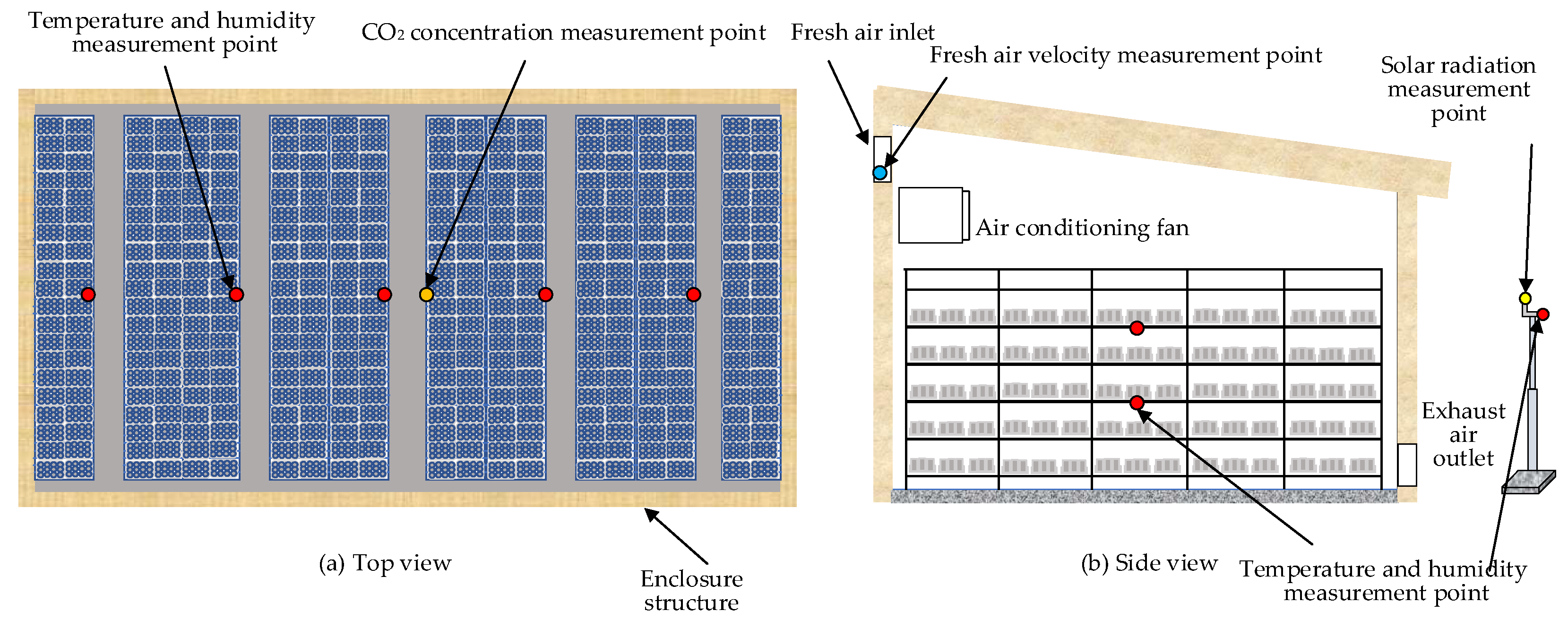
Figure 2.
Data processing process.
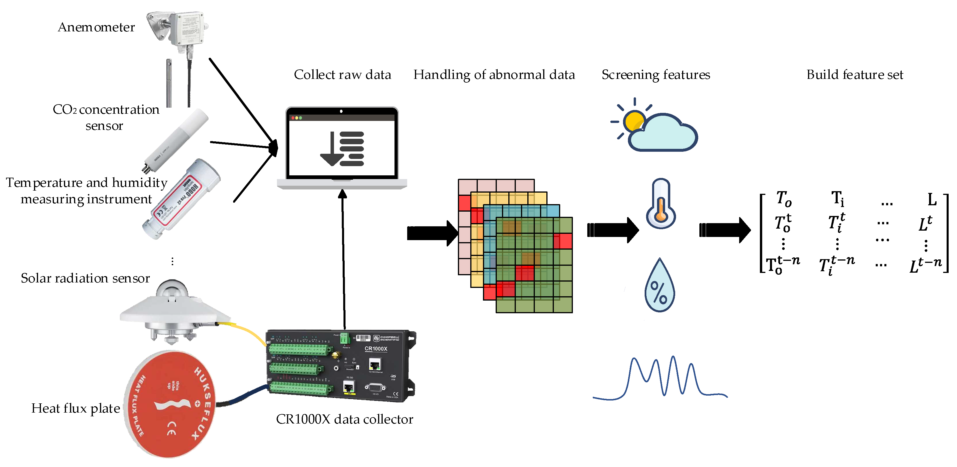
Figure 3.
Multiple experimental binomial distribution.
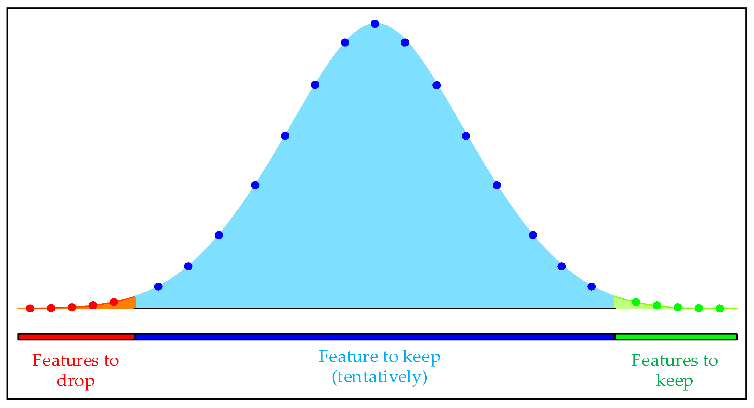
Figure 4.
Model prediction flow.
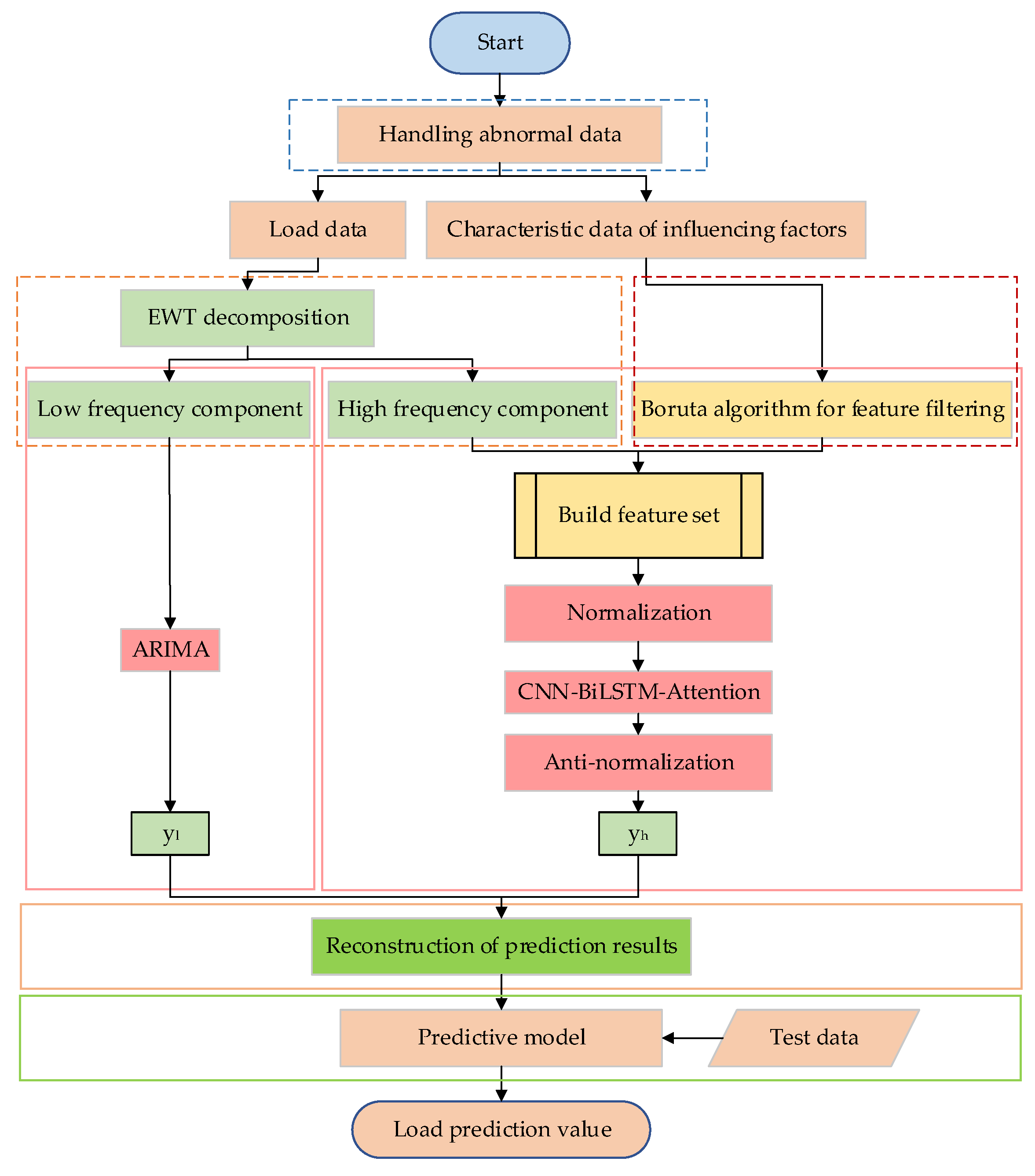
Figure 5.
Combined model structure of ARIMA and CNN-BiLSTM-Attention.
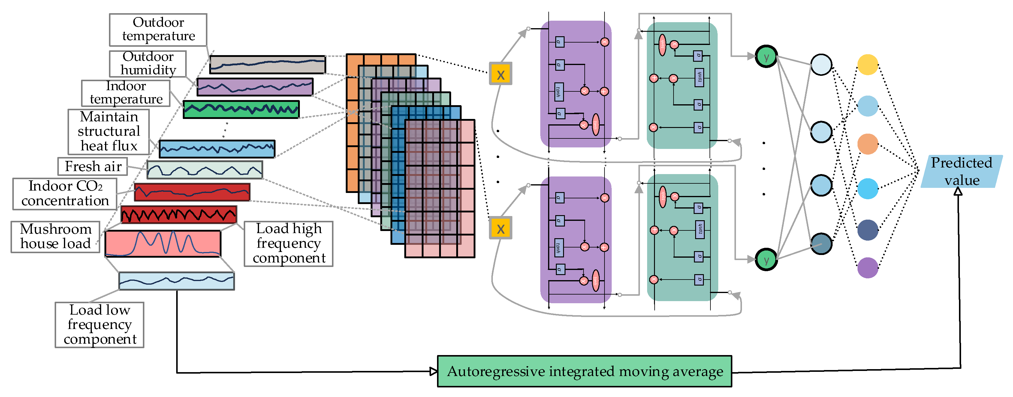
Figure 6.
Load curve of the mushroom house.
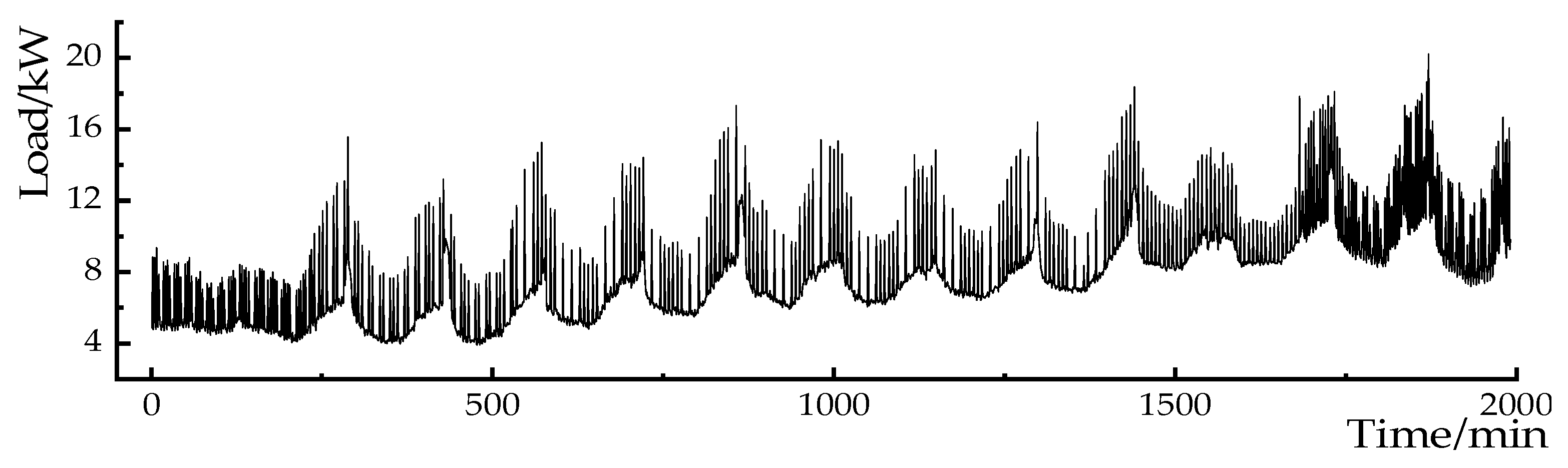
Figure 7.
Results of EWT decomposition of load data.
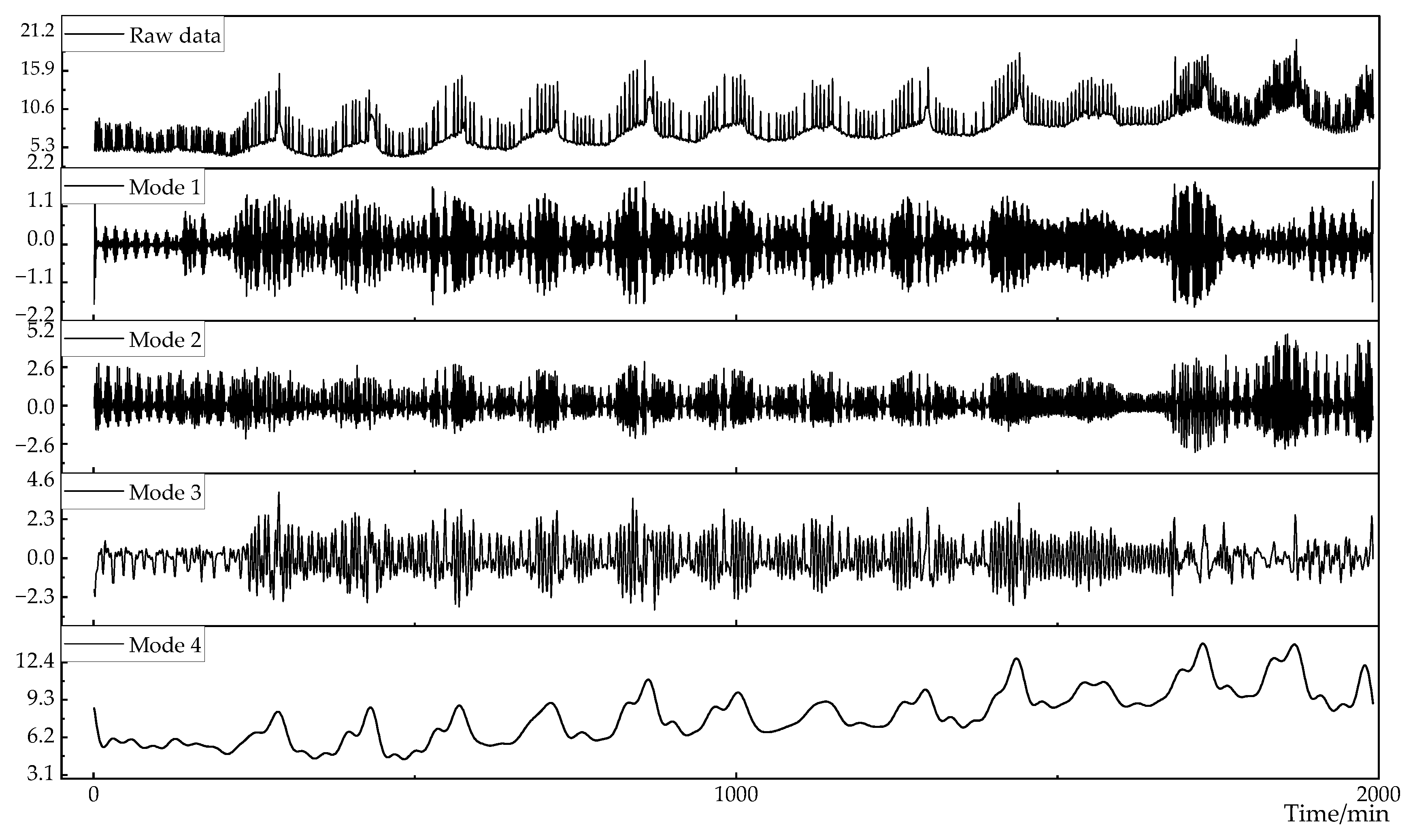
Figure 8.
Comparison of EWT and EEMD reconstruction errors.
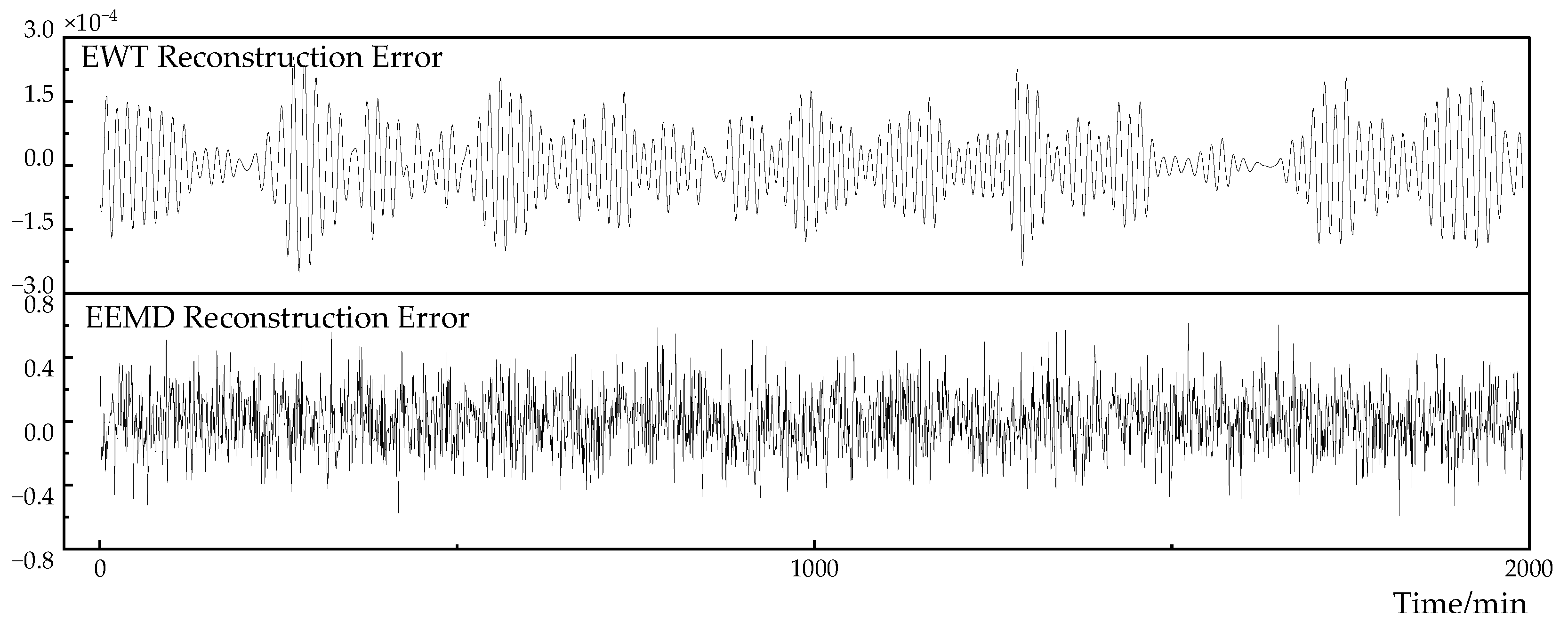
Figure 9.
Percentage of cumulative complexity for each mode.
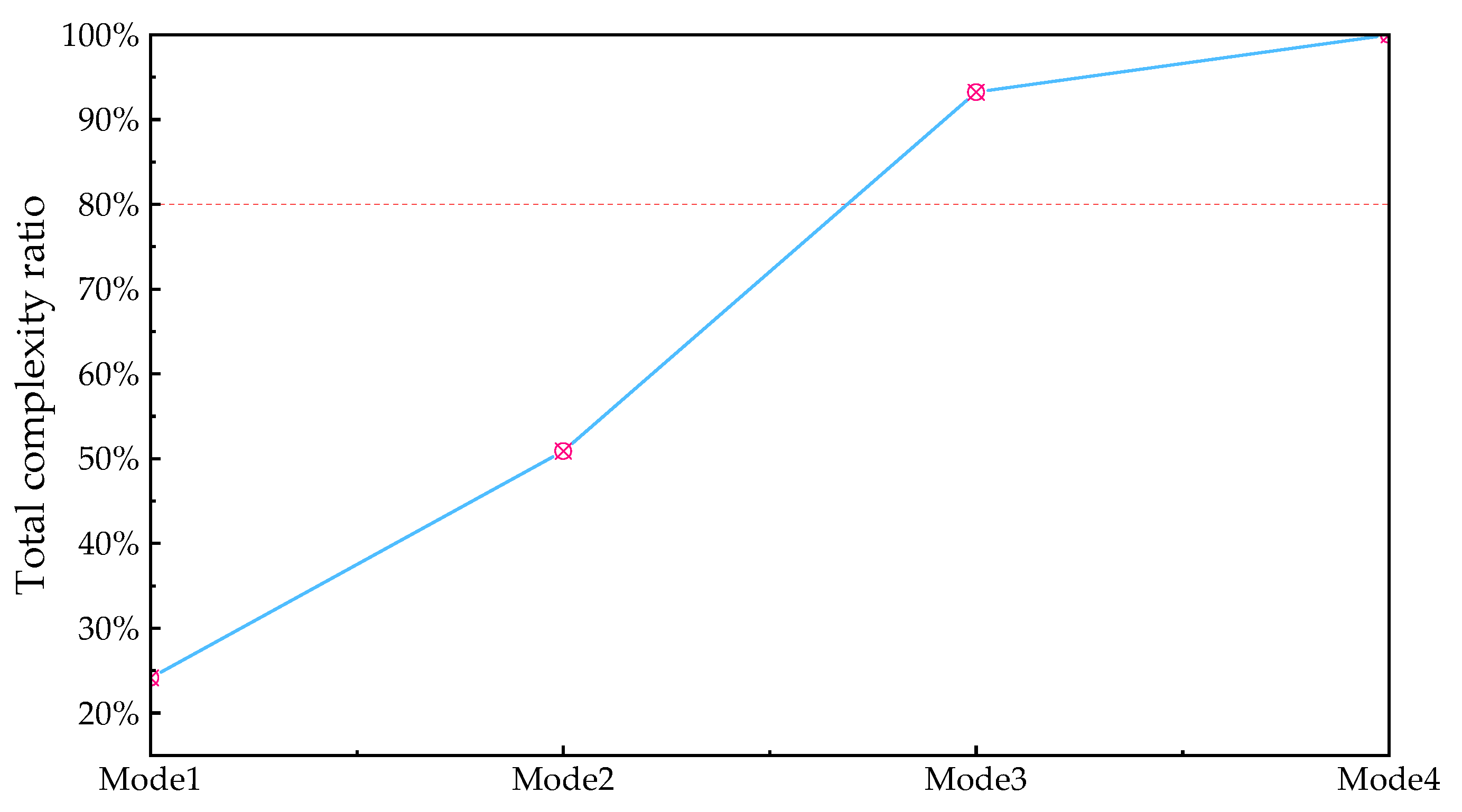
Figure 10.
EWT decomposition of load data.
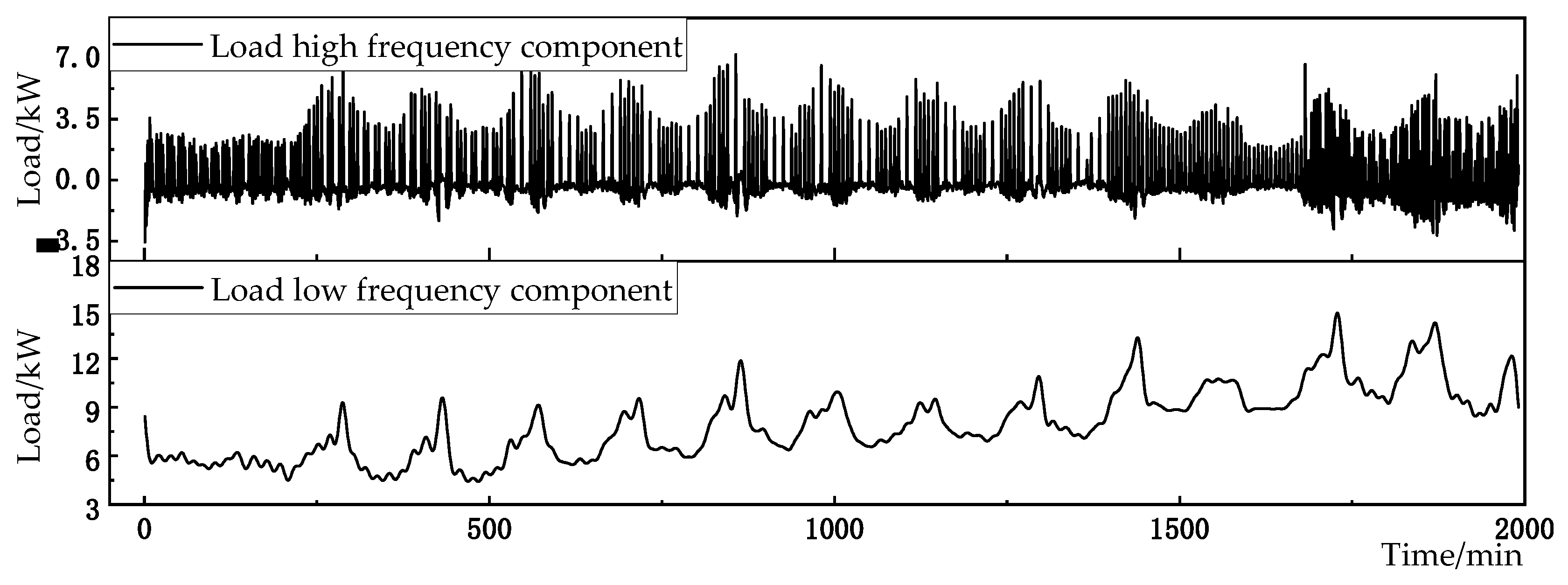
Figure 11.
Comparison of errors in prediction results between single and hybrid models.
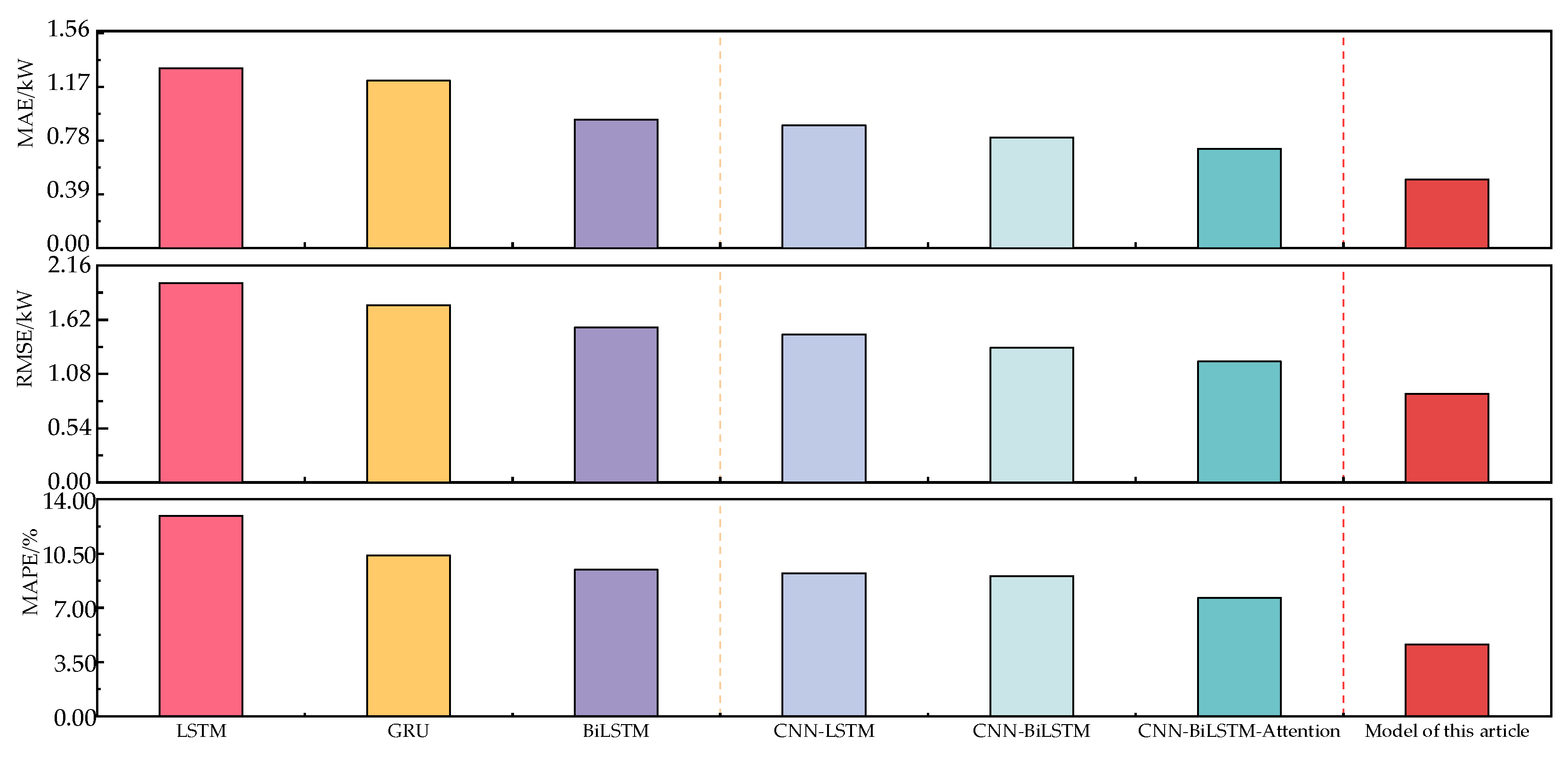

Table 1.
Characteristics of the collected data.
| Feature category | Feature name |
|---|---|
| Outdoor climate factors | Outdoor temperature |
| Outdoor humidity | |
| Solar radiation intensity | |
| Heat flux of the envelope | |
| Small indoor environmental factors | Indoor temperature |
| Indoor humidity | |
| Indoor CO2 concentration | |
| Equipment working status | Fresh air fan Air conditioner opening time |
Table 2.
Iterative process of feature screening algorithm Boruta.
| Number of iterations | Accept | Hesitant | Refuse |
|---|---|---|---|
| 1~8 | 0 | 8 | 0 |
| 9~36 | 7 | 1 | 0 |
| 37 | 7 | 0 | 1 |
| 38 | 7 | 0 | 1 |
Table 3.
Results of different feature screening methods.
| Feature screening method | Model evaluation index | |||
|---|---|---|---|---|
| Boruta | 0.591 | 1.056 | 5.68 | 63 |
| Pearson | 0.614 | 1.218 | 6.03 | 65 |
| Spearman | 0.711 | 1.291 | 6.77 | 66 |
| original data | 0.711 | 1.291 | 6.77 | 66 |
Table 4.
Sum of the absolute errors of the different decomposition components.
| Number | Number of decomposition components | Sum of absolute errors/kW |
|---|---|---|
| 1 | 3 | 0.08789 |
| 2 | 4 | 0.05737 |
| 3 | 5 | 0.09755 |
| 4 | 6 | 0.59034 |
Table 5.
Algorithm optimization results and model prediction errors.
| Algorithm | Number of convolution cores (CNN) | Number of neurons (BiLSTM) | Model evaluation index | ||
|---|---|---|---|---|---|
| PSO | 26 | 140 | 0.583 | 1.140 | 5.59 |
| GA | 5 | 25 | 0.570 | 0.967 | 5.47 |
| NGSA-II | 15 | 64 | 0.557 | 0.884 | 5.26 |
Table 6.
Parameter setting of hybrid model.
| Module | Parameter type | Parameter setting |
|---|---|---|
| Input layer | Input data structure | [24,7] |
| CNN Layer (2 layers) | (1st layer) Number of convolution kernel | 15 |
| (1st layer) Convolution kernel size | 3*3 | |
| Pool layer size | 1*2 | |
| (2nd layer) Number of convolution kernel | 1 | |
| (2nd layer) Convolution kernel size | 3*3 | |
| BiLSTM layer | Number of neurons | 64 |
| ARIMA layer | Differential order | 1 |
| other | Dropout rate | 0.1 |
| Loss function | Segmented loss function |
Table 7.
Comparison of prediction errors with different types of loss functions.
| Loss function | Model evaluation index | |||
|---|---|---|---|---|
| MAE | 0.518 | 1.001 | 5.10 | 62 |
| MSE | 0.557 | 0.884 | 5.26 | 63 |
| Segmented loss function | 0.497 | 0.950 | 4.64 | 63 |
Disclaimer/Publisher’s Note: The statements, opinions and data contained in all publications are solely those of the individual author(s) and contributor(s) and not of MDPI and/or the editor(s). MDPI and/or the editor(s) disclaim responsibility for any injury to people or property resulting from any ideas, methods, instructions or products referred to in the content. |
© 2023 by the authors. Licensee MDPI, Basel, Switzerland. This article is an open access article distributed under the terms and conditions of the Creative Commons Attribution (CC BY) license (https://creativecommons.org/licenses/by/4.0/).
Copyright: This open access article is published under a Creative Commons CC BY 4.0 license, which permit the free download, distribution, and reuse, provided that the author and preprint are cited in any reuse.


