
Submitted:
05 September 2023
Posted:
06 September 2023
You are already at the latest version
Abstract
. This paper features an analysis of the relative effectiveness of a
variety of methods of modelling Realised Volatility (RV), namely:
the use of Gegenbaur processes in Auto-Regressive Moving Average format,
GARMA, as opposed to Heterogenous Auto-Regressive HAR models and simple rules of thumb. The analysis is applied to two data sets that feature the RV
of the S&P500 index, as sampled at 5 minute intervals, provided by
the Oxford Man RV database. The GARMA model does perform slightly
better than the HAR model, but both models are matched by a simple
rule of thumb regression model based on the application of lags of
squared, cubed and quartic, demeaned daily returns.
Keywords:
GARMA
; gegenbaur processes
; HAR models
; realised volatility
; rules of thumb
1. Introduction
Over the past 100 years considerable advances have been made in time series modelling. Yule (1926) and Slutsky(1927) developed the stochastic analysis of time series and developed the concepts of autoregressive (AR) and moving average (MA) models. Box and Jenkins (1970) suggested methods for applying autoregressive moving average (ARMA) or autoregressive integrated moving average (ARIMA) models to find the best fit of a time-series model to past values of a time series.
A contrary view of the approriateness of this approach has been promoted by Commandeur and Koopman (2007), who suggested that the BoxJenkins approach is fundamentally problematic. They have championed the adoption of alternative state-space methods to counter the contention that many real economic series are not truly stationary, despite differencing.
In the 1980′s attention switched to the consideration of the issues related to stationarity and non-stationary time series, fractional integration and cointegration. Granger and Joyeaux (1980) and Hosking (1981) focussed attention on fractionally integrated autoregressive moving average (ARFIMA or FARIMA) processes. Unit root testing to assess the stationarity of a time series became established via the application of the Dickey-Fuller test, following the work of Dickey and Fuller (1979).
Engle and Granger (1987) developed the concept of cointegration, whereby two time series might be individually integrated and non-stationary I(1), but some linear combination of them might possess a lower order of integration and be stationary, in which case the series are said to be cointegrated. Many of these conceptual developments have important applications to economic and financial time series, and to economic theory in these discipline areas.
One of the common features of many time series of financial data sets is that the variance of the series is not homoscedastic, and that these features concerned are autocorrelated. Engle (1982) developed the Autoregressive Conditional Heteroskedasticity (ARCH) model that incorporates all past error terms. It was generalised to GARCH by Bollerslev (1986) to include lagged term conditional volatility. In other words, GARCH predicts that the best indicator of future variance is a weighted average of long-run variance, the predicted variance for the current period, and any new information in this period, as captured by the squared residuals. GARCH models provide an estimate of the conditional variance of a financial price time series.
An alternative approach is to measure the variance directly from the observed values of the price series, these are referred to as being realised measures of volatility. Realised measures are theoretically sound, high frequency, nonparametric-based estimators of the variation of the price path of an asset, during the times at which the asset trades frequently on an exchange. The metrics were developed by Anderson et al. (2001), Anderson et al. (2003), and Barndorff-Nielsen and Shephard (2002).
The modelling of the variance of financial time series and the use of realised volatility (RV) is the focus of attention of this paper. In the empirical analysis we use RV 5-minute estimates from Oxford Man for S&P500 Index as the RV benchmark (see: https://realized.oxford-man.ox.ac.uk/data). Their database contains daily (close to close) financial returns, and a corresponding sequence of daily realised measures .
Corsi (2009, p 174) suggests “an additive cascade model of volatility components defined over different time periods. The volatility cascade leads to a simple AR-type model in the realized volatility with the feature of considering different volatility components realized over different time horizons and which he termed as being a “Heterogeneous Autoregressive model of Realized Volatility”. We make use of the Corsi (2009) HAR model to model realised volatility (RV) in some of the empirical tests included in this paper.
However, the main focus of this paper is the application of Gegenbaur processes to the modeling of realised volatility (RV). Gegenbauer processes were introduced by Hosking (1981) and further developed by Andel (1986), and Gray, Zhang and Woodward (1989, 1994). The latter proposed the class of time series models known as Gegenbauer ARMA, or as abbreviated, GARMA processes, which are the central focus in this paper.
In the current paper, we compare the effectiveness of GARMA models, as opposed to HAR models and other rules of thumb, based on de-meaned squared daily returns, as methods for modelling and forecasting daily 5-minute RV.
The paper is a further companion piece to two previous studies in the topic’s general area, namely, Allen and McAleer (2020) and Allen (2020), that compared the effectiveness of stochastic volatility, vanilla GARCH and HAR models, as opposed to simple rules of thumb, in their effectiveness as tools for capturing the RV of major stock market indices.
The current paper concentrates on the S&P500 index, and examines whether GARMA, HAR or simple rules of thumb, better capture the RV sampled at 5-minute intervals, as provided by Oxford Man, of the S&P500 Index. Thus, the central concern is what is the best method of capturing the long memory properties of a historical time series of RV5 for the S&P500 index? This is in contrast with the two previously mentioned studies, which contrasted the effectiveness of the volatility models per se.
The benchmark is provided by the estimates of RV5 provided by Oxford Man, in a sample of daily estimates of realised volatility, RV5, running from 1997/05/08 until 2013/08/30 with 4096 observations, plus a longer-period sample of RV5, also based on the S&P500 Index, running from 2000/01/04 until 2020/04/30, comprising 5099 observations. This is the same data set as used in Allen (2020a).
The paper is motivated by Poon and Granger (2003, p. 507) who observed that: “as a rule of thumb, historical volatility methods work equally well compared with more sophisticated ARCH class and SV models.” This paper similarly seeks to explore whether simple rules of thumb, in this case based on the use of a regression model featuring squared demeaned daily returns, with a subsequent addition of cubed and quartic powers of them, perform as well as more sophisticated time series models.
2. Previous work and econometric models
Recent reviews of the literature on the nature and applications of Gegenbaur processes are provided by Hunt et al. (2021) and Dissanayake et al., (2018). Peiris, Allen and Peiris (2005), and Peiris and Thavaneswaran (2007), considered long memory models driven by heteroskedastic GARCH errors. Peiris and Asai (2016), returned to this topic, whilst Geugan (2020), combined Gegenbauer processes with integrated GARCH (GIGARCH), to include the attributes of long memory, seasonality and heteroskedasticity at the same time, in the modelling of volatility.
2.1. The basic GEGENBAUR model
Let be a stationary random process with the autocovariance and the autocorrelation function where . The spectral density function (sdf) is denoted by:
where is the Fourier frequency.
There are various ways in which the long memory component of the Gegenbaur model can be specified, as discussed in Dissanayake et al., (2018). In the analysis that follows, we utilise the R package garma, as developed by Hunt (2022).
A Gegenbaur process is a long memory process generated by the dynamic equation:
where and is a short memory process characterised by a positive and bounded spectral density . If (1) is a Gegenbaur process of order or a GARMA process. Dissanayake et al., (2018) mention that (1) complies with the definition of a long memory process at the frequency . According to (1), arises from filtering the process by the infinite impulse response filter:
It can be shown that a stationary Gegenbauer process contains an unbounded spectrum at and is long memory when . This special frequency is called the Gegenbauer or G-frequency, Dissayanake et al., (2018, p.416).
The GARMA model as fit by the garma package, Hunt (2022), is specified as:
- where represents the short-memory Autoregressive component of order
- represents the short memory Moving Average component of order
- represents the long-memory Gegenbauer component (there may in general be k of these),
- represents integer differencing (currently only = 0 or 1 is supported),
- represents the observed process,
- represents the random component of the model - these are assumed to be uncorrelated but identically distributed variates,
- represents the Backshift operator, defined by
When then this is just a short memory model, as would be represented by an ARIMA model.
2.2. Heterogenous Autoregressive Model (HAR)
Corsi (2009, p 174) suggests “an additive cascade model of volatility components defined over different time periods. The volatility cascade leads to a simple AR-type model in the realized volatility with the feature of considering different volatility components realized over different time horizons and which he termed as a Heterogeneous Autoregressive model of Realized Volatility”. Corsi (2009) suggests his model can reproduce the main empirical features of financial returns (long memory, fat tails, and self-similarity) in a parsimonious way. He writes his model as:
where is the daily integrated volatility, and and are respectively the daily, weekly, and monthly (ex post) observed realized volatilities.
2.3. Historical volatility model
Poon and Granger (2005) discuss various practical issues involved in forecasting volatility. They suggest that the HISVOL model has the following form:
where is the expected standard deviation at time , is the weight parameter, and is the historical standard deviation for periods indicated by the subscripts. Poon and Granger (2005) suggest that this group of models include the random walk, historical averages, autoregressive (fractionally integrated) moving average, and various forms of exponential smoothing that depend on the weight parameter .
We use a simple form of this model in which the estimate of is the previous day’s demeaned squared return. Poon and Granger (2005) review 66 previous studies and suggest that implied standard deviations appear to perform best, followed by historical volatility and GARCH which have roughly equal performance.
Barndorff-Neilsen and Shephard (2003) point out that taking the sums of squares of increments of log-prices has a long tradition in the financial economics literature. See for example, Poterba and Summers (1986), Schwert (1989), Taylor and Xu (1997), Christensen and Prabhala (1998), Dacorogna et al. (1998), and Andersen et al. (2001). Shephard and Sheppard (2009, p 200, footnote 4) note that: “Of course, the most basic realised measure is the squared daily return”. We utilise this approach as the basis of our historical volatility model. Furthermore, Perron and Shi (2020) show how the squared low-frequency returns can be expressed in terms of the temporal aggregation of a high-frequency series in relation to volatility measures.
3. Results
3.1. The data sets
To expedite a direct comparison with previous work on the HAR model we use the R library package ’HARModel’ by Sjoerup (2019). This contains data featuring realized measures from the SP500 index from April 1997 to August 2013, and we use the RV5, or realised measures on the S&P500 Index sampled at 5 minute intervals.
Table 1 provides a statistical description of this RV5 data set, together with that of another, slightly longer data set, taken from 2000 to 2020, also featuring S&P500 index RV5 data, taken from Allen and McAleer (2020a). Both of these data sets feature RV5 estimates taken from the Oxford Man Realized library, (https://realized.oxford-man.ox.ac.uk/).
One of the features of estimates of RV is that the data time series displays long-memory characteristics. Long memory refers to the association between observations in a time series are ever larger sample intervalling, and is also referred to as long-range dependence. It basically refers to the level of statistical dependence between two points in the time series sampled at increasing intervals.
Figure 1 displays the long memory characteristics of the two RV5 time series that we analyse. The first panel in the two plots displays the basic series of RV5 and the two large spikes in RV5, correspond to the effects on volatility of the Global Financial Crisis (GFC), that occurred in 2008. The two panels marked ACF and PACF, refer to the autocorrelation and partial autocorrelation statistics.
The R garma package, Hunt (2022), was used to generate the two graphs. The program was instructed to use 100 lags of daily observations. The blue lines in the bottom two sets of panels display the standard error bands. The long memory properties of RV5 are apparent in both sets of diagrams, in that the ACF statistics remains well outside the error bands for 100 lags, and the PACF is outside the error bands for up to 30 lags.
These long memory characteristics are used in Corsi’s (2009) HAR model and will be a feature of the Gegenbaur models that we fit to the data sets.
3.2. The basic HAR model
Table 2 provides summary descriptions of the HAR models fitted to the two RV5 data sets and Figure 2 provides plots of the fits. The results presented in Table 2 show that the basic HAR model does an excellent job in capturing the time series properties of RV5. All the estimates are significant at a one percent level, as are the F statistics, and the Adjusted R-squares are 52 percent, for the period 1997-2013, and 56 percent for the period 2000-2020, respectively.
The plots in Figure 2 confirm this, but do suggest that the large periodic peaks in RV5 are not captured so effectively by the HAR model. The question remains as to whether the Gegenbaur model will perform more effectively?
3.3. Gegenbaur results
The R library package (garma), Hunt (2022), was used to fit garma models to the realised volatility (RV) series sampled at 5 minutes for the S&P500 index as sourced from the OxfordMan library. This shorter RV series, for the S&P500 from 1997-2013, was taken from the HARmodel R library package, Sjoerup (2019).
A detailed summary of the methods used in the garma package are available in Hunt (2022). The garma package provides the ability to fit stationary, univariate GARMA models to a time series, and to forecast from those models. The garma() function in the garma package is the main function for estimating the parameters of a GARMA model. It provides three methods of parameter estimation - the Whittle method, (Whittle, (1953)), the conditional sum-of-squares (CSS) method, (for a discussion, See Hunt (2022) Ph.D, chapter 2, equation 2.3.2) and the WLLS method. The latter, Whittle Log Least-Squares method, was proposed by Hunt (2022, chapter3). The Whittle method was used in the estimations reported in the paper.
A summary of the Gegenbaur model estimated for this data is shown in Table 3. A potential advantage of the Gegenbaur model is that it is non-linear and more flexible than the HAR model.
The results of a regression of the fit from the Gegenbaur model for this data on the actual RV5 estimates for the S&P500 index for this period is shown in Table 4. The HAR model regression for this period, shown in the first half of Table 2, had an Adjusted R-squared of 0.52. The result for the Gegenbaur model estimation is an Adjusted R-squared of 0.567, and so the non-linear model does show an increased explanatory power.
We also fitted the Gegenbaur model to the longer time-period of RV estimates running from 2000 to 2020.

Table 5.
Gegenbaur estimation for RV5 for the S&P500 from 2000-2020, constant included with no trend.
Table 5.
Gegenbaur estimation for RV5 for the S&P500 from 2000-2020, constant included with no trend.
| Series | Intercept | U1 | fd1 | ar1 | ar2 | ar3 | ar4 | ar5 |
|---|---|---|---|---|---|---|---|---|
| coefficient | 1.175 | 0.9776774 | 0.12974 | 0.09841 | 0.18564 | -0.06645 | 0.11861 | 0.1606 |
| S.E. | 8.315 | 0.0004903 | 0.03286 | 0.06504 | 0.02608 | 0.01162 | 0.01376 | 0.0119 |
| Series | ar6 | ar7 | ar8 | ar9 | ar10 | ar11 | ar12 | ar13 |
| coefficient | -0.01016 | -0.02717 | 0.02901 | 0.23708 | -0.02952 | 0.01219 | 0.05422 | 0.05570 |
| S.E. | 0.01662 | 0.01295 | 0.01187 | 0.01259 | 0.02260 | 0.01466 | 0.01351 | 0.01408 |
| Series | ar14 | ar15 | ar16 | ar17Table | ar18 | ar19 | ar20 | |
| coefficient | -0.02716 | 0.05100 | 0.05079 | -0.04578 | -0.03084 | 0.01445 | 0.04350 | |
| S.E. | 0.01417 | 0.01183 | 0.01241 | 0.01240 | 0.01136 | 0.01165 | 0.01133 | |
| Series | Gegenbaur Frequency | Gegenbaur period | Gegenbaur Exponent | |||||
| coefficient | 0.0337 | 29.6812 | 0.1297 |
We regressed the actual daily RV5 series for the longer period from 2000 to 2020 and the results are shown in Table 6. The slope coefficient is significant at the 1 per cent level and is very close to 1, whilst the Adjusted R-square is 0.59 and the F statistics for the regression, with a value of 7326, is also significant at the 1 percent level. The Adjusted R-square for the HAR model for the same period was 0.56, so the Gegenbaur model provides a marginally better fit than the HAR model.
3.4. How do rule of thumb approaches perform?
The next issue is how do squared de-meaned end of day returns perform as a simple rule of thumb to explain RV5. Table 7 presents the results of the regression of RV5 for the longer period of 2000 to 2020 on 20 lags of squared demeaned daily returns.
It can be seen in Table 7 that 20 lags of squared demeaned returns do not perform quite as well as the Gegenbaur or HAR models but still have an Adjusted R-Square of 54 percent which is a marginal 2 percent less than the HAR model and 5 percent less than the Gegenbaur model. Only 4 of the 20 lags used in this rule of thumb approach are insignificant. The Durbin Watson statistic of 1.43 suggests that a considerable amount of autocorrelation remains in the residuals.
The application of Ramsey Reset tests suggest that squares and cubes of the explanatory variable could add to the power of the regression. Table 8 reports the results of adding 10 lags of cubed demeaned SPRET and 10 lags of demeaned SPRET to the power 4.
This is essentially another non-linear model, but admittedly we now have 40 explanatory variables in the model in the form of lags of three explanatory variables. The Adjusted R-Square now increases to over 59 percent which matches the power of the Gegenbaur model. Admittedly, the Durbin Watson statistic is still a relatively low 1.54. This suggests that there is still autocorrelation in the residuals which could be exploited further in enhanced modifications of the model.
4. Conclusion
In this paper we have explored the use of the Gegenbaur process or GARMA model to capture the behaviour of realised volatility of the S&P500 index sampled at 5 minute intervals, as reported by the OxfordMAN database. The results suggest that the non-linear Gegenbaur model does perform slightly better than the HAR model in capturing RV5. However, a simplified rule of thumb model based on the use of lagged, squared, cubed, and quartic, demeaned daily returns, performed equally well. These results, for the S&P500 index, suggest that non-linear models perform better than linear ones in the capture of long memory properties of RV5 and that sophisticated models do not necessarily dominate rules of thumb.
Author Contributions
Conceptualization, Allen. and Peiris; methodology, Allen and Peiris.; software, Allen and Peiris; validation, Allen and Peiris.; formal analysis, Allen.; investigation, Allen.; resources, Peiris.; data curation, Allen; writing—original draft preparation, Allen.; writing—review and editing, Allen and Peiris.; visualization, Allen.; project administration, Peiris.; funding acquisition, Peiris. All authors have read and agreed to the published version of the manuscript.
Funding
This research received no external funding.
Data Availability Statement
Index data was obtained from Yahoofinance. The Realised volatility data was originally obtained from OxfordMan at http://realized.oxford-man.ox.ac.uk, but this data base has recently been removed from public availability.
Conflicts of Interest
“The authors declare no conflict of interest.”
References
- Allen, D.E. 2020a. Stochastic volatility and GARCH: Do squared end-of-day returns provide similar information? Journal of Risk and Financial Management.13, 202. [CrossRef]
- Allen, D.E. and M. McAleer. 2020b. Do we need stochastic volatility and Generalised Autoregressive Conditional Heteroscedasticity? Comparing squared end-of-day returns on FTSE. Risks. 8, 12. [CrossRef]
- Andel, J. 1986. Long memory time series models. Kybernetika, 22: 105-123.
- Andersen, T.G., T. Bollerslev, F.X. Diebold, and H. Ebens. (2001), The distribution of realized stock return volatility, Journal of Financial Economics, 61: 43-76. [CrossRef]
- Andersen, T.G., T. Bollerslev, F.X. Diebold and P. Labys 2003. Modeling and forecasting realized volatility. Econometrica. 71: 529-626. [CrossRef]
- Barndorff-Nielsen, O.E. and N. Shephard. 2002. Econometric analysis of realised volatility and its use in estimating stochastic volatility models. Journal of the Royal Statistical Society, Series B. 63: 253-280.
- Barndorff-Nielsen, O.E. and N. Shephard. 2003. Realized power variation and stochastic volatility models. Bernoulli, 9(2):243-265. [CrossRef]
- Box, G. E. P. and G.M. Jenkins. 1970). Times Series Analysis. Forecasting and Control. Holden-Day, San Francisco, CA.
- Bollerslev, T. 1990. Modelling the coherence in short-run nominal exchange rates: A multivariate generalized ARCH model, Review of Economics and Statistics. 72, 498-505. [CrossRef]
- Christensen, B.J. and N.R. Prabhala. 1998. The relation between implied and realized volatility. Journal of Financial Economics. 37: 125-150. [CrossRef]
- Commandeur, J.J.F., and S.J. Koopman. 2007. Introduction to State Space Time Series Analysis. Oxford University Press. [CrossRef]
- Corsi, F. 2009. A simple approximate long-memory model of realized volatility. Journal of Financial Econometrics. 7(2): 174-196.
- Dacorogna, M.M., U.A. Muller, R.B. Olsen, and O.V. Pictet. 1998. Modelling short term volatility with GARCH and HARCH, in C. Dunis and B. Zhou (eds), Nonlinear Modelling of High Frequency Financial Time Series. Chichester, Wiley.
- Dickey, D. A. and W.A. Fuller. 1979. Distribution of the Estimators for Autoregressive Time Series with a Unit Root. Journal of the American Statistical Association. 74 (366): 427-431. [CrossRef]
- Dissanayake, D.S., S. Peiris, and T. Proietti. 2018. Fractionally Differenced Gegenbauer Processes with Long Memory: A Review. Statistical Science. 33, No. 3: 413-426. [CrossRef]
- Engle, R.F. 1982. Autoregressive conditional heteroskedasticity with estimates of the variance of United Kingdom inflation. Econometrica. 50: 987-1007. [CrossRef]
- Engle, R. F., and C.W. Granger. 1987. Co-integration and error correction: Representation, estimation and testing. Econometrica. 55 (2) 251-276. [CrossRef]
- Granger, C. W. J. and R. Joyeux. 1980. An introduction to long-memory time series models and fractional differencing. Journal of Time Series Analysis, 1: 15-29. [CrossRef]
- Gray, H. L., Zhang, N.F. and Woodward. 1989. On generalized fractional processes. Journal of Time Series Analysis, (10): 233-257. [CrossRef]
- Gray, H. L., Zhang, N.F. and Woodward. 1994. A correction: “On generalized fractional processes”. Journal of Time Series Analysis, 10 (1989), no. 3, 233. Journal of Time Series Analysis. 15: 561-562.
- Guegan, D. 2000. A new model: The k-factor GIGARCH process. Journal of Signal Processing. (4): 265-271.
- Hosking, J. R. M.. 1981. Fractional differencing. Biometrika. 68, 165-176. [CrossRef]
- Hunt, R., S. Peiris, and N. Weber. 2021. Estimation methods for stationary Gegenbauer processes. Statistical Papers. [CrossRef]
- Hunt, R.. 2022. garma: Fitting and Forecasting Gegenbauer ARMA Time Series Models, R package version 0.9.11. https://CRAN.R-project.org/package=garma.
- Hunt, R.. 2022. Investigations into Seasonal ARMA processes. PhD thesis submitted to the School of Mathematics and Statistics, University of Sydney, Sydney, NSW.
- Peiris, S., D. E. Allen, and U. Peiris. 2005. Generalized autoregressive models with conditional heteroscedasticity: An application to financial time series modeling. In Proceedings of the Workshop on Research Methods: Statistics and Finance. 75-83.
- Peiris, S., and M. Asai. 2016. Generalized fractional processes with long memory and time dependent volatility revisited. Econometrics. 4(3), 37. [CrossRef]
- Perron, Pierre, and Wendong Shi. 2020. Temporal aggregation and Long Memory for asset price volatility. Journal of Risk and Financial Management. 13: 181. [CrossRef]
- Poon, S-H., and C.W. T. Granger. 2005. Practical issues in forecasting volatility. Financial Analysts Journal. 61: 45-56. [CrossRef]
- Poterba, J. and L. Summers. 1986. The persistence of volatility and stock market fluctuations. American Economic Review. 76: 1124-1141. [CrossRef]
- Ramsey, J. B. 1969. Tests for Specification Errors in Classical Linear Least Squares Regression Analysis. Journal of the Royal Statistical Society, Series B. 31 (2): 350–371. [CrossRef]
- Schwert, G.W. 1989. Why does stock market volatility change over time? Journal of Finance. 44: 1115-1153. [CrossRef]
- Shephard, N., and K. Sheppard. 2010. Realising the future: Forecasting with high-frequency-based volatility (HEAVY) models. Journal of Applied Econometrics. (25): 197-231. [CrossRef]
- Sjoerup, E. 2019. HARModel: Heterogeneous Autoregressive Models. R package version 1.0. https://CRAN.R-project.org/package=HARModel.
- Slutsky, E.H. 1927. The summation of random causes as the source of cyclic processes. Econometrica. 5: 105 - 146.
- Taylor, S.J. and X. Xu. 1997. The incremental volatility information in one million foreign exchange quotations. Journal of Empirical Finance. 4: 317-340. [CrossRef]
- Whittle, P. 1953. The analysis of multiple stationary time series. Journal of the Royal Statistical Society. Series B (Methodological). 15(1):125. [CrossRef]
- Yule, G.U. 1926. Why do we sometimes get nonsense correlations between timeseries? a study in sampling and the nature of time-series. Journal of the Royal Statistical Society. 89: 1 - 63. [CrossRef]
Figure 1.
Plots of the RV5 samples for the S&P500 index and their long-range dependence.
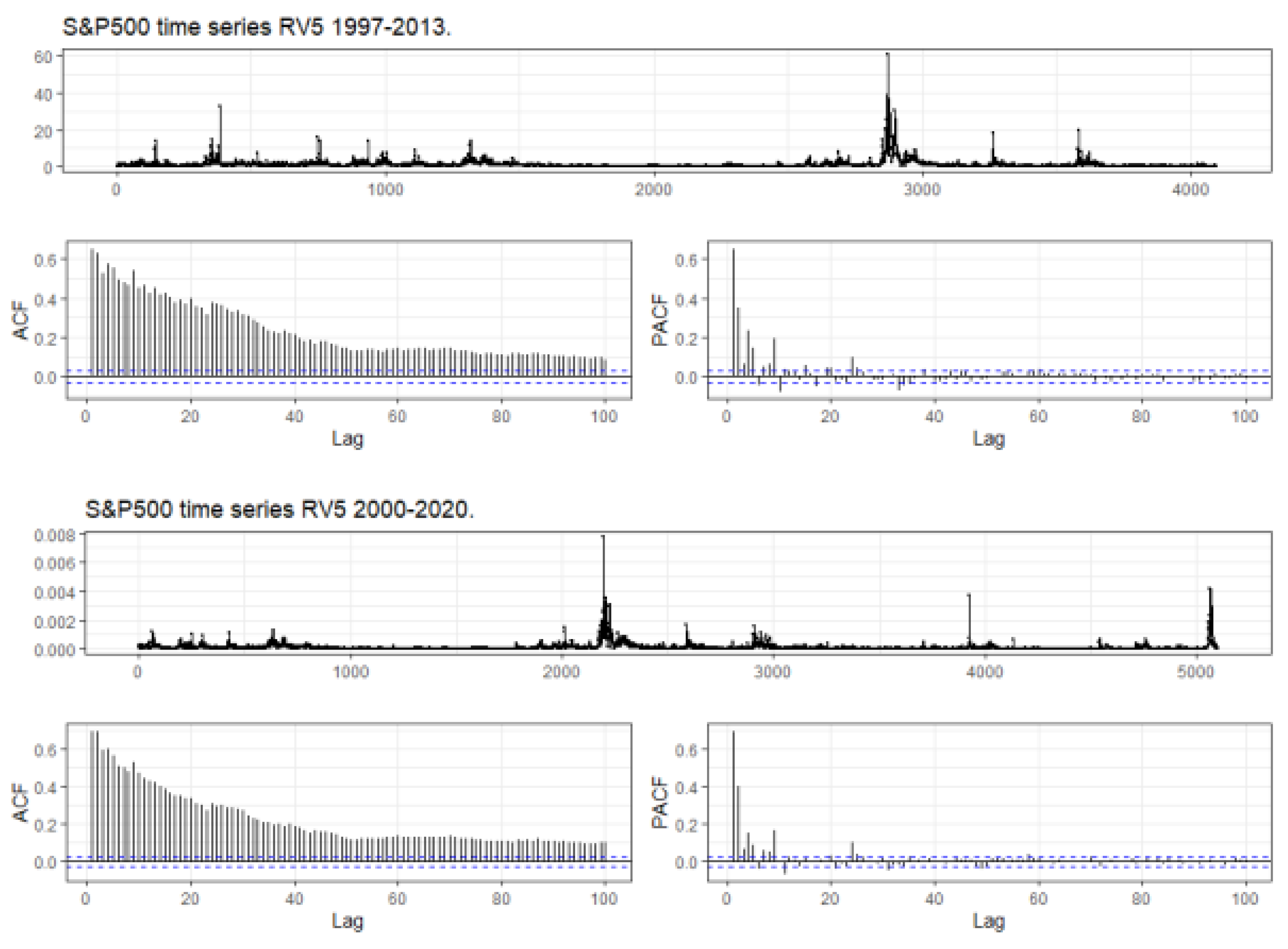
Figure 2.
Plots of Fitted HAR Models.
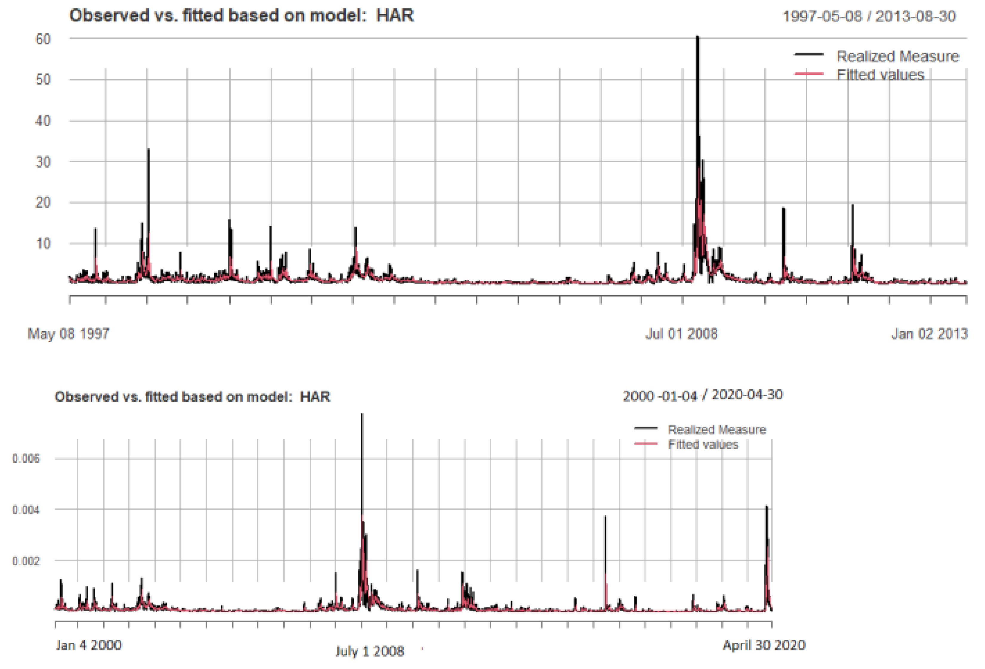
Table 1.
Descriptive Statistics RV5 data sets.
| Descriptor | S&P500 1997-2013 | S&P500 2000- 2020 |
|---|---|---|
| Number of Observations | 4096 | 5099 |
| Minimum | 0.04329 | 0.00000122 |
| Maximum | 60.56 | 0.0074 |
| median | 0.6294 | 0.0000471 |
| mean | 1.1752 | 0.000112 |
| Standard Deviation | 2.3151 | 0.000269 |
NB: The data taken from the R library package HARModel on RV5 was scaled up in the package.
Table 2.
Summary of the HAR models fitted to the RV5 data sets.
| S&P500 1997-2013 RV5 | ||||||
|---|---|---|---|---|---|---|
| Coefficient | Estimate | Standard Error | t. value | |||
| beta0 | 0.11231 | 0.03065 | 3.664*** | |||
| beta1 | 0.22734 | 0.01870 | 12.157*** | |||
| beta5 | 0.49035 | 0.03144 | 15.595*** | |||
| beta22 | 0.18638 | 0.02813 | 6.624 *** | |||
| Adjusted R-squared | 0.5221 | |||||
| F-Statistic | 1484*** | |||||
| S&P500 2000-2020 RV5 | ||||||
| Coefficient | Estimate | Standard Error | t. value | |||
| beta0 | 1.218e-05 | 2.877e-06 | 4.235*** | |||
| beta1 | 2.703e-01 | 1.704e-02 | 15.858*** | |||
| beta5 | 5.295e-01 | 2.633e-02 | 20.108 *** | |||
| beta22 | 9.134e-02 | 2.225e-02 | 4.105*** | |||
| Adjusted R-squared | 0.5608 | |||||
| F-Statistic | 2162*** | |||||
Note: *** Indicates significant at the 1% level.
Table 3.
Gegenbaur estimation for RV5 for the S&P500 from 1997-2013, constant included with no trend.
Table 3.
Gegenbaur estimation for RV5 for the S&P500 from 1997-2013, constant included with no trend.
| Series | Intercept | U1 | fd1 | ar1 | ar2 | ar3 | ar4 | ar5 |
|---|---|---|---|---|---|---|---|---|
| coefficient | 1.139e-04 | 0.9794239 | 0.33368 | -0.27435 | 2.215e-11 | -5.991e-11 | 0.09145 | 0.08230 |
| S.E. | 7.430e-08 | 0.0001457 | 0.03893 | 0.07677 | 5.745e-02 | 3.259e-02 | 0.02167 | 0.01137 |
| Series | ar6 | ar7 | ar8 | ar9 | ar10 | ar11 | ar12 | ar13 |
| coefficient | -0.02743 | 9.408e-11 | 0.02743 | 0.2469 | 0.16461 | 0.08230 | 0.1097 | 0.10974 |
| S.E. | 0.01075 | 1.034e-02 | 0.01050 | 0.0118 | 0.02678 | 0.02949 | 0.0260 | 0.02663 |
| Series | ar14 | ar15 | ar16 | ar17 | ar18 | ar19 | ar20 | ar21 |
| coefficient | 0.02743 | 0.0823 | 0.0823 | 0.02743 | 1.320e-10 | 1.125e-10 | -6.332e-12 | -0.03658 |
| S.E. | 0.02655 | 0.0205 | 0.0208 | 0.02007 | 1.578e-02 | 1.237e-02 | 1.103e-02 | 0.01056 |
| Series | ar22 | ar23 | ar24 | ar25 | ar26 | ar27 | ar28 | ar29 |
| coefficient | -0.02743 | -0.10974 | 0.04572 | -0.02743 | -0.02743 | 0.02743 | 4.256e-11 | -4.386e-11 |
| S.E. | 0.01127 | 0.01226 | 0.01763 | 0.01204 | 0.01327 | 0.01359 | 1.129e-02 | 1.117e-02 |
| Series | ar30 | Gegenbaur frequency | Gegenbaur period | Gegenbaur Exponent | ||||
| coefficient | 0.02743 | 0.0323 | 30.9197 | 0.3337 | ||||
| S.E. | 0.01050 |
Table 4.
Regression of RV5 on Gegenbaur model estimates, 1997-2013.
| Coefficient | S.E. | |
|---|---|---|
| Constant | 0.0003596 | 0.0287058 |
| RV5 | 0.9994219*** | 0.0136477 |
| Adjusted RSQ | 0.567 | |
| F. Statistic | 5363 |
Note: *** Indicates significant at the 1% level.
Table 6.
Regression of RV5 on Gegenbaur model estimates, 2000-2020.
| Coefficient | S.E. | |
|---|---|---|
| Constant | 6.72543e-07 | 2.77936e-06 |
| RV5 | 0.993054 *** | 0.0116015 |
| Adjusted RSQ | 0.589660 | |
| F. Statistic | 7326.850 *** |
Note: *** Indicates significant at the 1% level.
Table 7.
Regression of RV5 on squared demeaned daily returns for 2000 to 2020. OLS, using observations 21–5099 ( = 5079) Dependent variable: rv5
Table 7.
Regression of RV5 on squared demeaned daily returns for 2000 to 2020. OLS, using observations 21–5099 ( = 5079) Dependent variable: rv5
| . | Coefficient | Std. Error | -ratio | p-value | ||||
| const | 3 | 02614e–005 | 2 | 84505e–006 | 10 | 64 | 0 | 0000 |
| SQSPRET_1 | 0 | 174294 | 0 | 00555060 | 31 | 40 | 0 | 0000 |
| SQSPRET_2 | 0 | 0935967 | 0 | 00558548 | 16 | 76 | 0 | 0000 |
| SQSPRET_3 | 0 | 0527928 | 0 | 00587581 | 8 | 985 | 0 | 0000 |
| SQSPRET_4 | 0 | 0280810 | 0 | 00587693 | 4 | 778 | 0 | 0000 |
| SQSPRET_5 | 0 | 0591188 | 0 | 00587284 | 10 | 07 | 0 | 0000 |
| SQSPRET_6 | 0 | 0386591 | 0 | 00589632 | 6 | 556 | 0 | 0000 |
| SQSPRET_7 | 0 | 0127360 | 0 | 00592375 | 2 | 150 | 0 | 0316 |
| SQSPRET_8 | 0 | 0125674 | 0 | 00590739 | 2 | 127 | 0 | 0334 |
| SQSPRET_9 | 0 | 0460141 | 0 | 00590538 | 7 | 792 | 0 | 0000 |
| SQSPRET_10 | 0 | 0109619 | 0 | 00588044 | 1 | 864 | 0 | 0624 |
| SQSPRET_11 | 0 | 0125986 | 0 | 00588112 | 2 | 142 | 0 | 0322 |
| SQSPRET_12 | 0 | 00679795 | 0 | 00590660 | 1 | 151 | 0 | 2498 |
| SQSPRET_13 | 0 | 000835242 | 0 | 00590814 | 0 | 1414 | 0 | 8876 |
| SQSPRET_14 | 0 | 00784497 | 0 | 00592586 | 1 | 324 | 0 | 1856 |
| SQSPRET_15 | 0 | 00255057 | 0 | 00589736 | 0 | 4325 | 0 | 6654 |
| SQSPRET_16 | 0 | 0109373 | 0 | 00587609 | 1 | 861 | 0 | 0628 |
| SQSPRET_17 | 0 | 00499043 | 0 | 00587928 | 0 | 8488 | 0 | 3960 |
| SQSPRET_18 | 0 | 0124227 | 0 | 00592245 | 2 | 098 | 0 | 0360 |
| SQSPRET_19 | 0 | 0124595 | 0 | 00563006 | 2 | 213 | 0 | 0269 |
| SQSPRET_20 | 0 | 00716919 | 0 | 00559011 | 1 | 282 | 0 | 1997 |
| Mean dependent var | 0.000112 | S.D. dependent var | 0.000269 | |||||
| Sum squared resid | 0.000168 | S.E. of regression | 0.000182 | |||||
| 0.543145 | 0.541339 | |||||||
| 300.6678 | ) | 0.000000 | ||||||
| Log-likelihood | 36531.92 | Akaike criterion | 73021.83 | |||||
| Schwarz criterion | 72884.64 | Hannan–Quinn | 72973.79 | |||||
| 0.281412 | Durbin–Watson | 1.437144 | ||||||
Table 8.
Regression of RV5 on squared, cubed and quartic daily demeaned returns for 2000 to 2020. OLS, using observations 21–5099 ( = 5079) variable: rv5
Table 8.
Regression of RV5 on squared, cubed and quartic daily demeaned returns for 2000 to 2020. OLS, using observations 21–5099 ( = 5079) variable: rv5
| .. | Coefficient | Std. Error | -ratio | p-value | ||||
| const | 4 | 82971e–006 | 3 | 03009e–006 | 1 | 594 | 0 | 1110 |
| SQSPRET_1 | 0 | 231351 | 0 | 00958455 | 24 | 14 | 0 | 0000 |
| SQSPRET_2 | 0 | 110377 | 0 | 00959229 | 11 | 51 | 0 | 0000 |
| SQSPRET_3 | 0 | 118282 | 0 | 00966599 | 12 | 24 | 0 | 0000 |
| SQSPRET_4 | 0 | 0666821 | 0 | 00969419 | 6 | 879 | 0 | 0000 |
| SQSPRET_5 | 0 | 0642053 | 0 | 00980063 | 6 | 551 | 0 | 0000 |
| SQSPRET_6 | 0 | 0669488 | 0 | 00989797 | 6 | 764 | 0 | 0000 |
| SQSPRET_7 | 0 | 0345805 | 0 | 00995553 | 3 | 473 | 0 | 0005 |
| SQSPRET_8 | 0 | 0169334 | 0 | 00994948 | 1 | 702 | 0 | 0888 |
| SQSPRET_9 | 0 | 0254747 | 0 | 00993460 | 2 | 564 | 0 | 0104 |
| SQSPRET_10 | 0 | 0227310 | 0 | 00975198 | 2 | 331 | 0 | 0198 |
| SQSPRET_11 | 0 | 00478774 | 0 | 00583425 | 0 | 8206 | 0 | 4119 |
| SQSPRET_12 | 0 | 0213587 | 0 | 00588183 | 3 | 631 | 0 | 0003 |
| SQSPRET_13 | 0 | 00934631 | 0 | 00582412 | 1 | 605 | 0 | 1086 |
| SQSPRET_14 | 0 | 00178946 | 0 | 00578095 | 0 | 3095 | 0 | 7569 |
| SQSPRET_15 | 0 | 000564490 | 0 | 00574051 | 0 | 09833 | 0 | 9217 |
| SQSPRET_16 | 0 | 00229510 | 0 | 00575739 | 0 | 3986 | 0 | 6902 |
| SQSPRET_17 | 0 | 00247291 | 0 | 00572209 | 0 | 4322 | 0 | 6656 |
| SQSPRET_18 | 0 | 00617666 | 0 | 00576039 | 1 | 072 | 0 | 2837 |
| SQSPRET_19 | 0 | 00692568 | 0 | 00554060 | 1 | 250 | 0 | 2114 |
| SQSPRET_20 | 0 | 0188372 | 0 | 00539186 | 3 | 494 | 0 | 0005 |
| CUSPRET_1 | 0 | 534907 | 0 | 0592631 | 9 | 026 | 0 | 0000 |
| CUSPRET_2 | 0 | 574605 | 0 | 0614957 | 9 | 344 | 0 | 0000 |
| CUSPRET_3 | 0 | 542658 | 0 | 0625408 | 8 | 677 | 0 | 0000 |
| CUSPRET_4 | 0 | 421881 | 0 | 0625029 | 6 | 750 | 0 | 0000 |
| CUSPRET_5 | 0 | 581211 | 0 | 0623480 | 9 | 322 | 0 | 0000 |
| CUSPRET_6 | 0 | 406321 | 0 | 0625585 | 6 | 495 | 0 | 0000 |
| CUSPRET_7 | 0 | 306419 | 0 | 0622486 | 4 | 923 | 0 | 0000 |
| CUSPRET_8 | 0 | 0728304 | 0 | 0624320 | 1 | 167 | 0 | 2434 |
| CUSPRET_9 | 0 | 0440999 | 0 | 0614311 | 0 | 7179 | 0 | 4729 |
| CUSPRET_10 | 0 | 143643 | 0 | 0603871 | 2 | 379 | 0 | 0174 |
| sq_SQSPRET_1 | 11 | 1016 | 0 | 991204 | 11 | 20 | 0 | 0000 |
| sq_SQSPRET_2 | 5 | 00005 | 0 | 992337 | 5 | 039 | 0 | 0000 |
| sq_SQSPRET_3 | 10 | 1474 | 1 | 01023 | 10 | 04 | 0 | 0000 |
| sq_SQSPRET_4 | 7 | 20797 | 1 | 01302 | 7 | 115 | 0 | 0000 |
| sq_SQSPRET_5 | 2 | 06748 | 1 | 01765 | 2 | 032 | 0 | 0422 |
| sq_SQSPRET_6 | 5 | 51711 | 1 | 01948 | 5 | 412 | 0 | 0000 |
| sq_SQSPRET_7 | 4 | 90765 | 1 | 02938 | 4 | 768 | 0 | 0000 |
| sq_SQSPRET_8 | 0 | 981766 | 1 | 03193 | 0 | 9514 | 0 | 3415 |
| sq_SQSPRET_9 | 2 | 00887 | 1 | 02378 | 1 | 962 | 0 | 0498 |
| sq_SQSPRET_10 | 2 | 40620 | 1 | 00723 | 2 | 389 | 0 | 0169 |
| Mean dependent var | 0.000112 | S.D. dependent var | 0.000269 | |||||
| Sum squared resid | 0.000148 | S.E. of regression | 0.000172 | |||||
| 0.596908 | Adjusted | 0.593707 | ||||||
| 186.5095 | P-value() | 0.000000 | ||||||
| Log-likelihood | 36849.86 | Akaike criterion | 73617.72 | |||||
| Schwarz criterion | 73349.87 | Hannan–Quinn | 73523.92 | |||||
| 0.228344 | Durbin–Watson | 1.543216 | ||||||
Disclaimer/Publisher’s Note: The statements, opinions and data contained in all publications are solely those of the individual author(s) and contributor(s) and not of MDPI and/or the editor(s). MDPI and/or the editor(s) disclaim responsibility for any injury to people or property resulting from any ideas, methods, instructions or products referred to in the content. |
© 2023 by the authors. Licensee MDPI, Basel, Switzerland. This article is an open access article distributed under the terms and conditions of the Creative Commons Attribution (CC BY) license (http://creativecommons.org/licenses/by/4.0/).
Copyright: This open access article is published under a Creative Commons CC BY 4.0 license, which permit the free download, distribution, and reuse, provided that the author and preprint are cited in any reuse.


