1. Introduction
The current space environment situational awareness[
1,
2,
3,
4,
5],near-Earth asteroid detection [
6], and large-scale sky survey [
7,
8] etc. yield massive amount of star image data every day. Star image registration is a fundamental data processing step for astronomical image differencing [
9], stacking [
10] and mosaicking [
11] applications, and has high requirements on the robustness, accuracy and real-time of the registration algorithm.
Image registration is a key and difficult problem in the field of image processing, which aims to register images of the same object acquired under different conditions using the computed inter-pixel transformation relations. Generally, image registration can be divided into three types: intensity-based registration algorithms, feature-based registration algorithms and neural network-based registration algorithms [
12]. The intensity-based image registration algorithm evaluates the intensity correlation of image pairs in the spatial or frequency domain, and is a classical statistical registration algorithm with representative algorithms including normalized cross-correlation (NCC) [
13,
14], mutual information [
15] and Fourier Merlin transform (FMT) [
16]. The advantages of intensity-based registration algorithms are that they do not require feature extraction and are simple to implement. The disadvantages are that they are computationally expensive and cannot be registered when the background changes drastically or when grayscale information is poor, which are unfortunately not uncommon in star images, and that the global optimal solution cannot be obtained in most cases using the similarity measure function. Feature-based registration algorithms correspond robust features extracted from image pairs [
17], which usually have better real-time and robustness, and have been a hot topic of research, which are mainly divided into feature descriptor-based and spatial distribution relationship-based algorithms. Feature descriptor-based registration algorithms include SIFT [
18,
19], SURF [
20,
21,
22], FAST [
23], ORB [
24] and others. To ensure the rotation invariance of the feature descriptors, most of these algorithms and their improved versions need to use the gradient information of the local regions of the feature points to determine the dominant orientation, but since the grayscale of the star image in astronomical images has the same gradient drop in each direction and the different local regions will produce different dominant orientations, this leads to the lack of robustness of these algorithms to rotation in star image registration applications. In addition FAST and ORB algorithms mainly detect corner points as feature points in the image, while corner points are almost non-existent in star images, so these algorithms are not applicable to this field. Spatial distribution relationship-based registration algorithms mainly include polygonal algorithms [
25,
26,
27] and grid algorithms [
28,
29]. Polygonal algorithms often cannot balance real-time and robustness, because it is obvious that the robustness is best to perform an exhaustive test for all combined point pairs, but their computational load is massive when there are many stars, which is often unacceptable in practical applications, so a trade-off between real-time and robustness is needed. Grid algorithms mostly use experience to determine the reference axis based on the brightness or angle of neighboring stars, and the performance deteriorates dramatically when the stars are dense or unreliable in brightness. Neural network-based registration algorithms are now widely studied in the field of remote sensing image registration, which can be broadly classified into two types of deep neural network-based [
30,
31,
32] and graph neural network-based [
33,
34]. The greatest advantage of deep neural networks is their powerful feature extraction ability especially for the advanced features, so the richer the image features the better the performance of deep neural network algorithms, but the star images lack conventional features such as color, texture, shape, etc., and advanced features are scarce, these characteristics determine that the registration algorithms based on deep neural networks are hardly applicable to this field. SuperPoint and SuperGlue (SPSG) combined algorithms are typical of graph neural network-based registration algorithms, SuperPoint is a network model that simultaneously extracts image feature points and descriptors, and SuperGlue is a feature registration network based on graph neural network and attention mechanism. The related registration algorithms incorporating SPSG have achieved excellent results in the CVPR Image Matching Challenge for three consecutive years from 2020 to 2022. Like the feature descriptor-based registration methods, the SPSG algorithm suffers from the same lack of robustness to rotation in star image registration applications, and its high performance and memory requirements on the GPU can limit its use in applications with limited hardware resources.
Challenges of star image registration include image rotation, insufficient overlapping area, false stars, position deviation, magnitude deviation, high-density stars and complex sky background, etc., and the high requirements of robustness, accuracy and real-time. This paper designs a high-precision robust real-time star image alignment algorithm by relying on the radial modulus feature and the rotation angle feature, and combining the characteristics that the relative distances of star pairs vary very little at different positions on the image, and using the voting strategy reasonably. The algorithm belongs to spatial distribution relationship-based registration algorithm, which is similar to the mechanism of animal recognition of stars [
35], and draws on the ideas of polar coordinate-based grid star map matching [
29] and voting strategy-based star map matching [
36]. A large number of simulated and real data test results show that the comprehensive performance of the proposed algorithm is significantly better than the four classical baseline algorithms when there are image rotation, insufficient overlap area, false stars, position deviation, magnitude deviation, high-density stars and complex sky background, and it is a more ideal star image registration algorithm.
The rest of this paper is structured as follows. In
Section 2, a brief description of the image preprocessing process used in this paper is given. In
Section 3, we describe in detail the principles and implementation steps of the proposed star image registration algorithm. In
Section 4 deals with the full and rigorous testing of the algorithm performance using simulated and real data, as well as the comparison with the classical baseline registration algorithms.
Section 5 discusses the comprehensive performance of star image registration algorithms. Finally,
Section 6 concludes the paper.
2. Image Preprocessing
2.1. Background Suppression
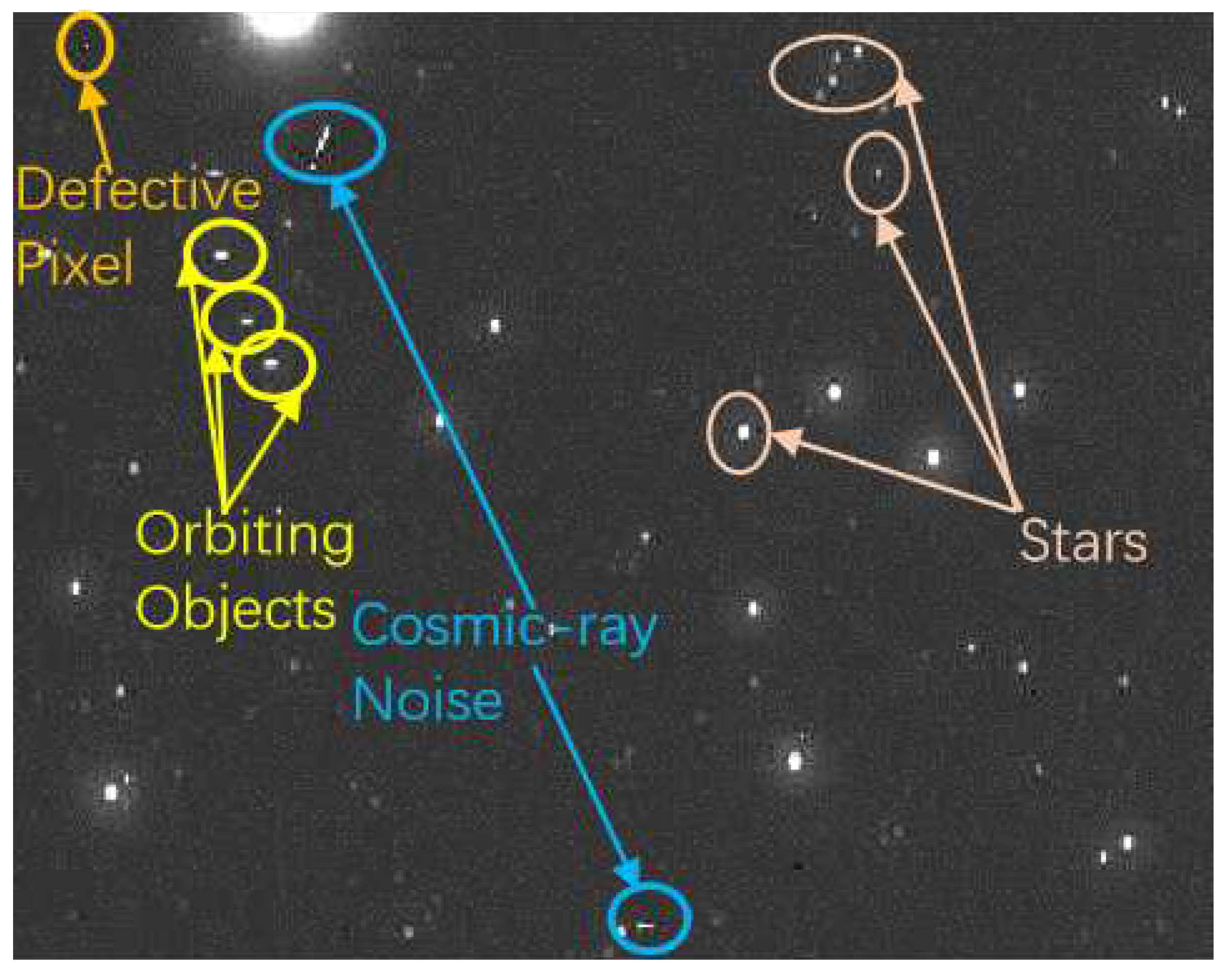
A typical star image is shown in
Figure 1, which consists of the four parts as shown in Equation (
1).
where
I denotes star image,
B denotes low-frequency undulating background such as mist, atmospheric glow, ground gas light, etc.,
S denotes stellar images,
O denotes near-Earth orbit object images such as satellites, debris, near-Earth asteroids, etc., and
N denotes high-frequency noise such as cosmic-ray noise, defective pixels, etc. According to the frequency characteristics, the composition of the star image can be divided into mainly low-frequency undulating background and mainly high-frequency stars, near-Earth orbit (NEO) objects and noise two categories. High-frequency noise and NEO objects are similar to the stellar image, so it is difficult to suppress them in the preprocessing stage. Therefore, in order to extract the stellar centroid as accurately as possible, the low-frequency undulating background should be suppressed first.
The effectiveness and real-time of morphological filtering have been well proven in the field of weak target detection [
37], so in this paper, the preprocessing step uses the morphological reconstruction [
38] algorithm to suppress the undulating background. The specific steps are to first obtain the marker image using Top-Hat filtering, as shown in Equation (
2).
where
I is the original image,
is the morphological open operator, and
is the structure element generally selected as a flat structure element of size 3 to 5 times the defocus blur diameter. To improve the positioning accuracy of the stellar centroid, telescopes are usually designed with defocus [
39], so that the single–pixel star image spreads into a bright spot, and the defocused blur diameter is the diameter of that bright spot.
Then the morphological reconstruction operation is executed, as shown in Equation (
3).
where
is the marker image in the iterative process,
is the morphological dilation operator,
is the structural element of the reconstruction process generally using 3×3 flat structural elements, and
indicates that the corresponding pixel takes a small value. Until the reconstruction process is stopped when
, at which point
is the estimated image background.
Finally, the estimated image background is subtracted from the original image to obtain the background–suppressed image, denoted as .
2.2. Stellar Centroid Positioning
The binary mask image is obtained by segmenting the image after background suppression using the adaptive threshold shown in Equation (
4).
where
and
are the mean and standard deviation of the image after background suppression, respectively, and
k is the adjustment coefficient, which takes the value of a real number from 0.5 to 1.5 in general.
Then the connected components with holes in the binary mask image is filled. The holes in the connected components may be caused by the bright star overexposure triggering the CCD gain protection mechanism resulting in a dark spot in the center of the star image, or a dead pixel right on the star image. After filling the holes, objects with too few pixels are removed. Objects with too few pixels are usually defective pixels or faint stars that cannot be precisely positioned and need to be eliminated if possible. Finally, the intensity-weighted centroid formula as shown in Equation (
5) is used to calculate the stellar centroid.
3. Star Image Registration
3.1. Matching Features
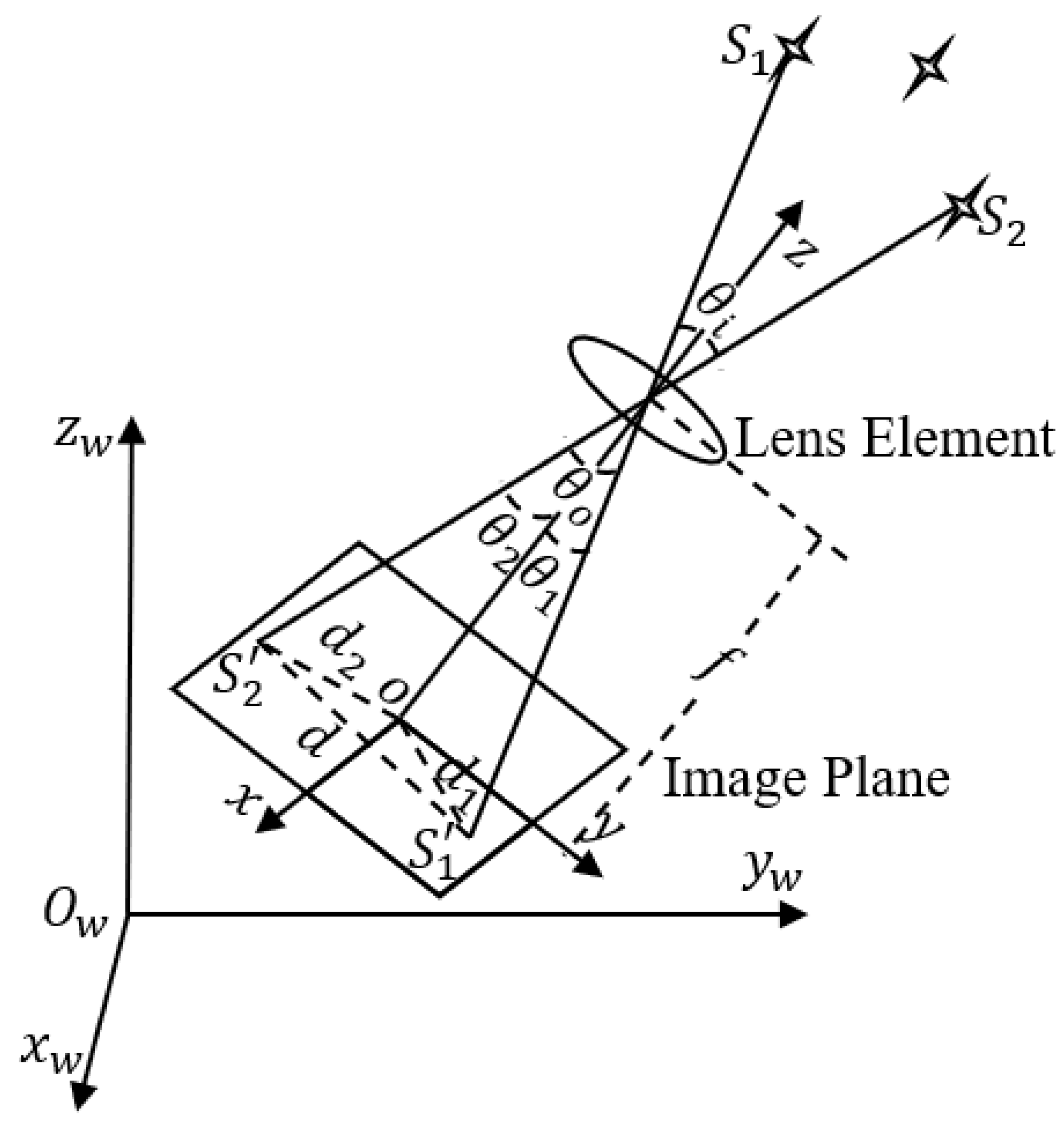
The stellar light is focused on the light-sensitive plane through the lens to form an image, and the imaging model can be regarded as a pinhole perspective projection model [
40], as shown in
Figure 2.
In
Figure 2,
is the world coordinate system and
is the camera coordinate system. According to the principle of pinhole imaging, the angle
is always holding, and because the star is a point source of light at infinite distance from the camera,
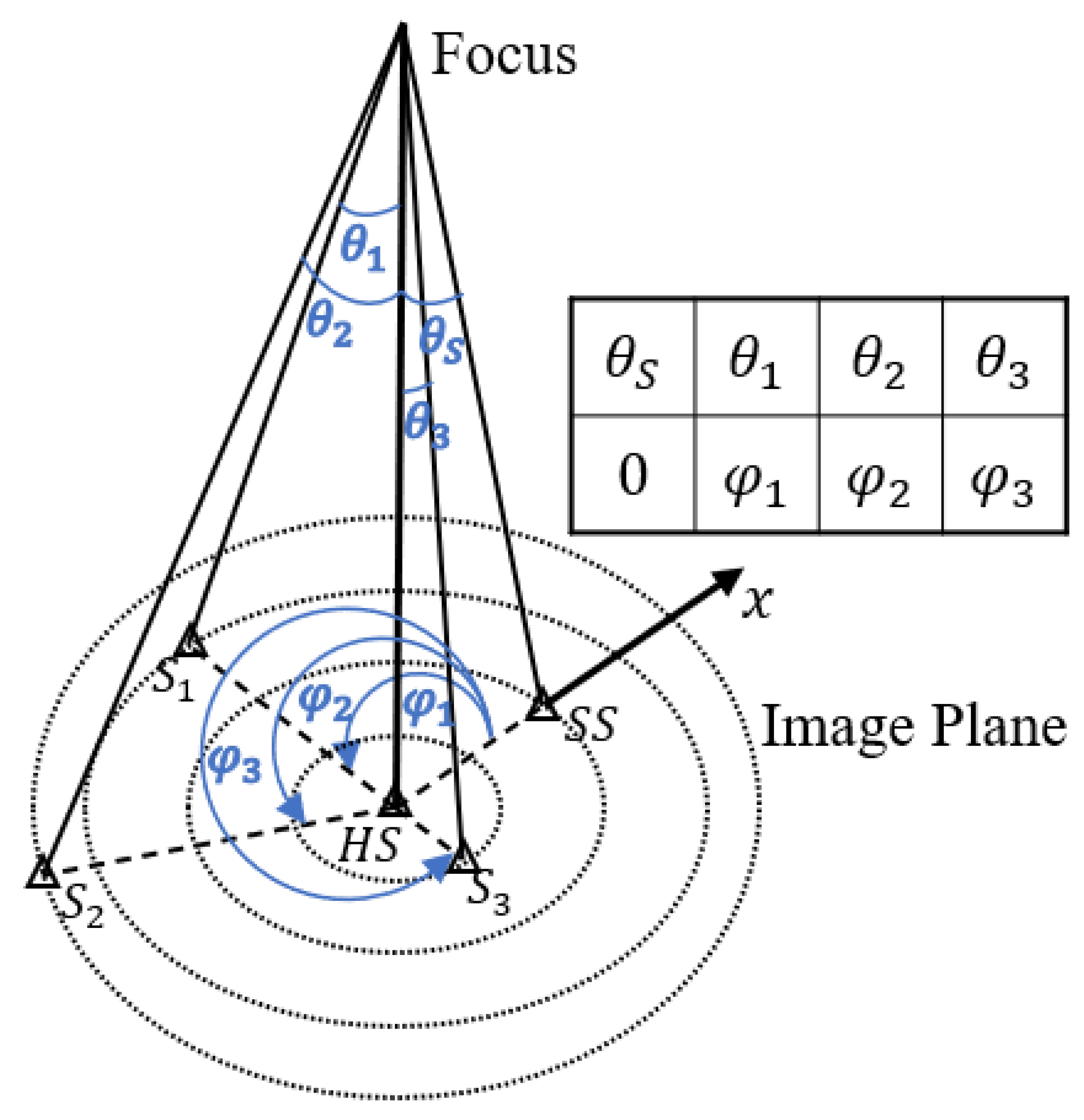
does not change with the movement of the camera. According to the above analysis, we can conclude that the angle between two stars is constant no matter when, where, and in what position they are photographed, so the angle between the stars is a good matching feature, which is called radial modulus feature (RMF) in this paper. The position of the star cannot be uniquely determined by using only the interstellar angles, so this paper adds a rotational angle feature – the angle of counterclockwise rotation of the reference axis formed by the host star (HS) and the starting star (SS) in the image plane to the line connecting the HS and the neighboring star, which is rotationally invariant when the HS and the SS are determined. The matching features of the HS are shown in
Figure 3.
Calculating the angle between stars requires introducing the focal length, and the focal length will vary due to temperature, mechanical vibration, etc. This will cause errors in the calculation of the angle, in order to avoid this error and to be able to directly use 2-dimensional coordinates to reduce the calculation, the distance between stars can also be used instead of the angle between stars as RMF. It should be noted that the distance between stars varies at different positions in the image, but by analysis this variation is acceptable in image registration for most astronomical telescopes. Let the field of view angle be
and the image size be
n pixels, the analysis process of this variation amount in combination with
Figure 2 is as follows.
When
the distance between stars takes the minimum value.
When
the distance between the stars takes the maximum value.
Then the maximum value of the variation when the angle is
is shown in equation (
9).
For a given field of view angle
and image size
n, the distance variation takes the maximum value when
.
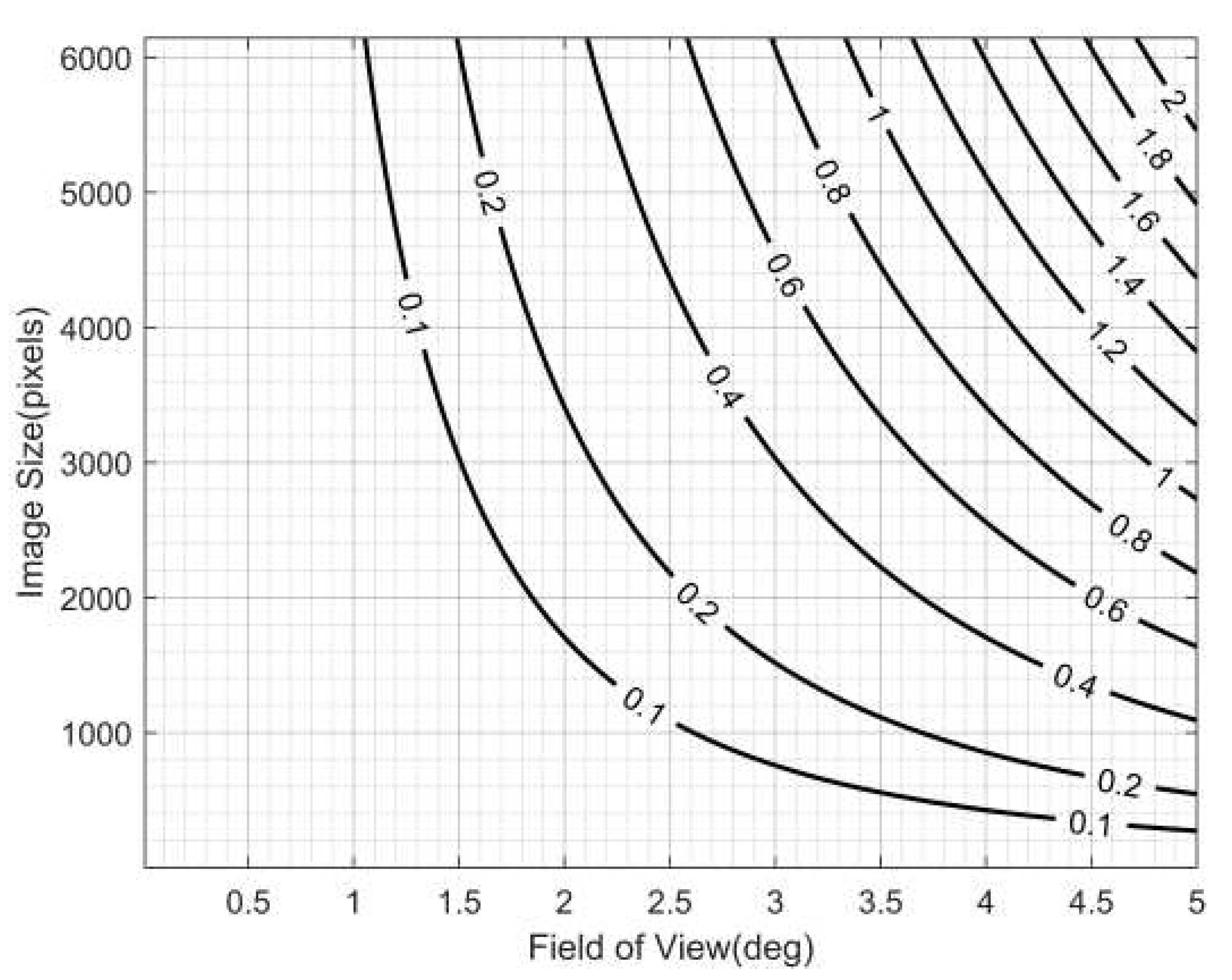
The relationship between the maximum distance variation and the field of view and image size is shown in
Figure 4.
Figure 4 or equation (
10) can be used as a reference for the subsequent adoption of angles between stars or distances between stars as RMF. For example, according to
Figure 4, for most astronomical telescopes with a field of view of less than 5 degrees, the effect of variations in the distance of the star pair at image different positions on the registration can be largely avoided by setting a suitable matching threshold. Of course, for very large field of view or ultra-high-resolution telescopes such as LSST, it is recommended to use the angle between stars as the RMF. These two choices are identical in the registration process except for the different methods of calculating the features, and the subsequent narrative of this paper will use the distance between the stars as the radial modal feature, as shown in
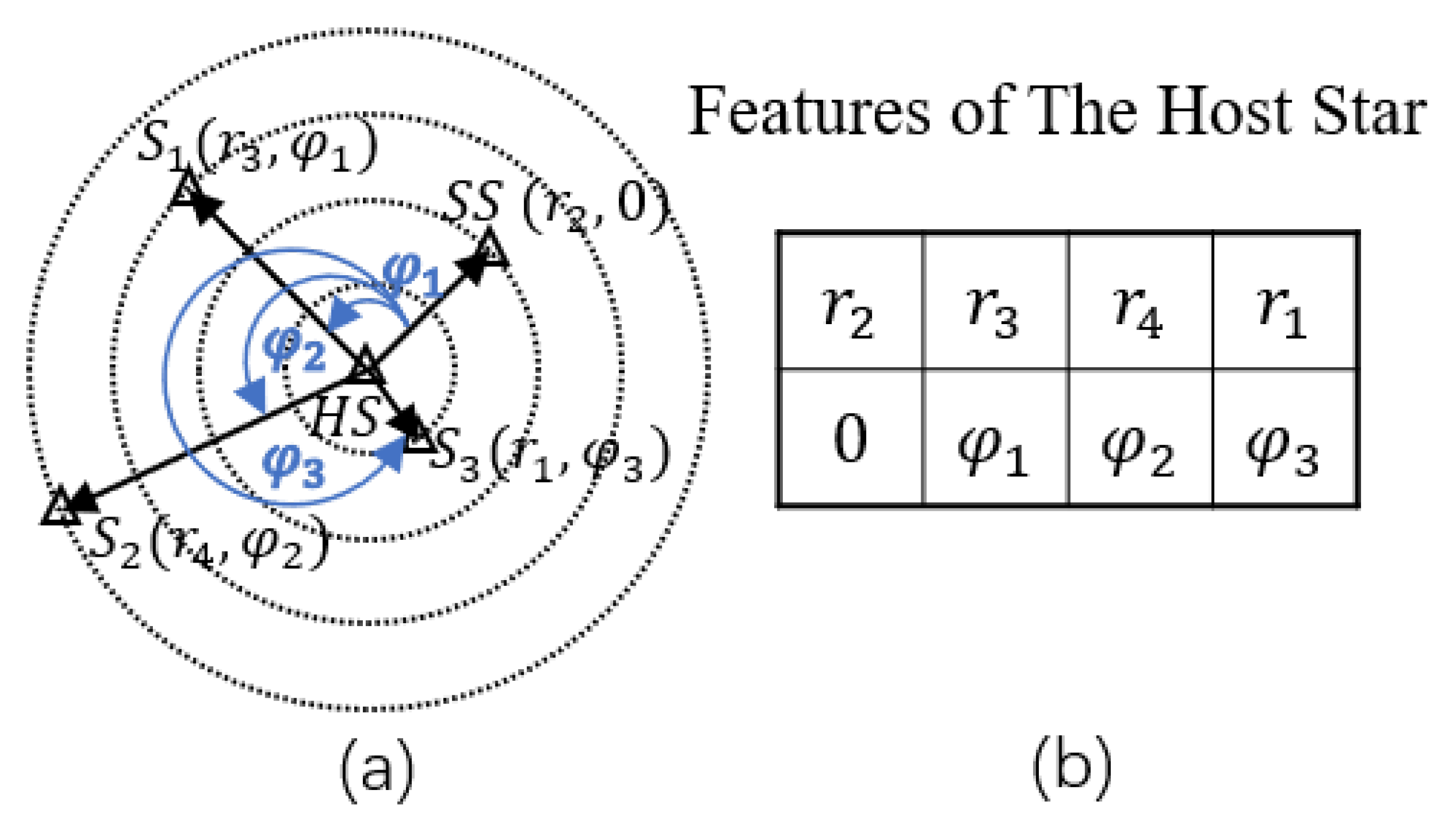
Figure 5.
As shown in
Figure 5a, the RMF of the HS refers to the distances of all neighboring stars to HS in the image plane, which is translational and rotationally invariant; the RAF still refers to the angle of counterclockwise rotation of the reference axis formed by the HS and the SS to the line connecting the HS and the neighboring stars in the image plane, because the distances of the star pairs at different positions in the image do not vary much, so the angle between the stars hardly varies with their positions, that is, the RAF is also translational and rotationally invariant when the SS is determined.
Figure 5b shows the feature list of the HS containing RMF and RAF. In summary, the RMF and the RAF can be used to uniquely determine the position of each neighboring star under the condition that the HS and the SS are determined, and it is easy to obtain matching stars with high confidence and low false match rate.
3.2. Registration Process
The registration process mainly consists of determining the candidate HS and SS and verifying them, and obtaining all matched stars to calculate transformation parameters. The details of the process are described below.
3.2.1. Calculating RMF and initial–RAF
The RMF of the stars in the moving image and the fixed image are calculated respectively, obtaining the RMF matrices
and
.
where
represents the Euclidean distance between the
star and the
star on the star image, and
and
denote the number of stars extracted in the moving image and the fixed image, respectively.
The initial-RAF (IRAF) of all stars in the moving image and the fixed image are calculated respectively, obtaining the IRAF matrices
and
.
where
represents the initial rotation angle of the
star when the
star is the HS, and it is specified that
when
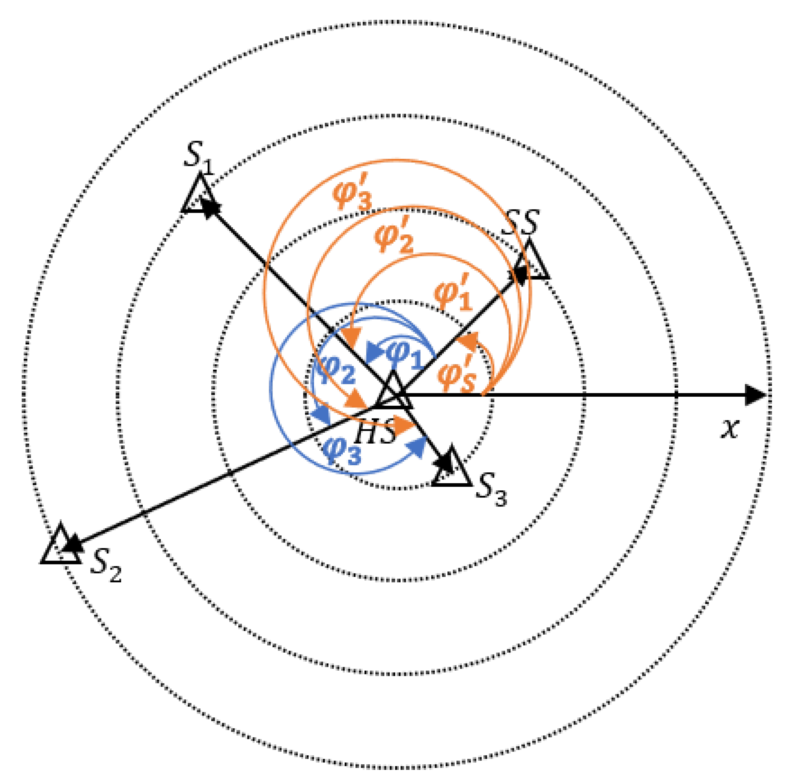
. The IRAF is the rotation angle calculated by using the image horizontal axis instead of the reference axis formed by the HS and the SS. As shown in
Figure 6, it differs from the RAF by a fixed angle, which is the angle of counterclockwise rotation of the image horizontal axis to the line connecting the HS and the SS, and the RAF is obtained by subtracting this angle directly from the IRAF after the SS is determined.
3.2.2. Determine the candidate HS and SS
The determination of the HS and the SS is to find two matching pairs of stars in the image pair to be registered, either one of which is the HS and the other is the SS, which is the most key step of the registration process in this paper. To ensure the robustness, a voting algorithm based on RMF is used to obtain the candidate HS and SS. The following is an example of the process of determining the candidate matching star in the fixed image for the star in the moving image.
The RMF
(row
i of
) of the
star in the moving image is taken, and its matching degree with the stars in the fixed image is counted separately, as shown in equation (
15).
where
denotes the base of the set, i.e., the number of elements. Due to that the distance between the stars is different at image different positions and the positioning error, the intersection operation here does not require the two elements to be exactly equal, as long as the difference between the two elements is within the set threshold value, the two elements are considered to be the same.
Considering the existence of false stars, noise and other interferences and that matching by RMF alone is not unique, therefore, in order to avoid missing the correct match as much as possible, all stars with matching degree greater than the threshold are selected here as candidate matching stars, and the set
of candidate matching stars in the fixed image is given by equation (
16).
where,
denotes the matching degree set. Select two different stars in the moving image as the HS and the SS, respectively, and determine the corresponding candidate HS and SS in the fixed image using the above candidate matching star determination method.
3.2.3. Verifying and obtaining matching star pairs
The candidate HS and SS combinations need to be rigorously verified to ensure that a sufficiently reliable correct combination is obtained, and the process needs to avoid unnecessary redundancy as much as possible to ensure real-time performance. Let the candidate HS and SS in the moving image be
and
, respectively, and the corresponding candidate matching HS and SS in the fixed image be
and
, respectively. First verify whether the distance difference between the HS and the SS in the moving image and the fixed image is less than the threshold value as shown in equation (
17). Although this step is simple, it can avoid a large number of incorrect combinations of the HS and the SS and strongly ensure the real-time performance.
where
and
denote the
and
features of the RMF of HS in the moving image and fixed image, respectively, which are also the distances between the HS and the SS.
If the initial test is passed, a secondary test is performed in combination with the RAF. In the IRAF matrices
and
of the moving image and fixed image, the IRAF
(row
of
) and
(row
of
) of the corresponding candidate HS are taken, respectively, and the RAF
and
are obtained by correcting the IRAF according to the candidate SS, as shown in equations (
18) and (
19).
So far, all matching features—RMF and RAF of the host star in the moving and fixed images have been obtained, as shown in equations (
20) and (
21).
where
and
represent the matching features of the HS in the moving image and the fixed image, respectively, which are equivalent to the set of neighboring star coordinates with the HS as the origin and the line connecting the HS and the SS as the polar axis. Calculate the pairwise Euclidean distances of the feature points in
and
to obtain the distance verification matrix.
where
denotes the distance between the
feature point in the moving image and the
feature point in the fixed image. The candidate matching marker matrix is obtained using equation (23).
where, the operator
is used to determine whether two elements are equal and its result is a Boolean value, and
is a logical AND operator. The matches in the candidate match matrix
obtained using the above method are all one-to-one. Finally, eliminating the candidate matches that are larger than the threshold using equation (
24) to get the match marker matrix.
If , it means the star in the moving image matches with the star in the fixed image, so the number of true in F is the number of matched star pairs. If the number of matched star pairs is greater than the matching threshold , the registration is judged to be successful; otherwise, the remaining combinations of candidate HS and SS will continue to be verified; if all combinations fail to pass the verification, the voting strategy will be used to determine the candidate matching stars for the remaining stars in the moving image, and the above steps will be repeated until verification is passed or there are no remaining stars in the moving image to be voted.
3.2.4. Maximum matching number registration
This step is performed when all stars in the moving image have been voted and still cannot pass the test. The reason for failing the test is not necessarily that the image pair cannot really be registered, but also that the matching threshold is set too large. To ensure the matching effect, is usually set appropriately large and proportional to the number of stars extracted, and when there are too many false stars in the extracted stars or insufficient overlapping areas between images, is likely to be set too large, resulting in failure to pass the test. To avoid this situation, this step is added in this paper, which is the last insurance to ensure the success of the registration and therefore plays a very important role in the robustness of the algorithm.
After each execution of the secondary test, the serial numbers of the HS and the SS in the moving image and the fixed image are recorded, as well as the corresponding number of matched star pairs. When all the stars in the moving image are voted and still cannot pass the test, the record with the highest number of matched star pairs is searched for, and if the number of matched star pairs in this record is greater than 3, the information of all matching star pairs is obtained using the aforementioned algorithm as the final matching result.
3.2.5. Calculating transformation parameters
Most feature-based registration algorithms use the strategy of first rough matching and then optimally rejecting the mis–matching points [
41], the algorithm in this paper obtains matched star pairs with high confidence and low mis–matching rate therefore the step of rejecting the mis–matching is not needed and the transformation parameters can be calculated directly.
In this paper, the Homography transformation model [
25,
40]is used and the transformation parameters between the moving image and the fixed image are solved using the Total Least Square (TLS) method. If the right-angle coordinates of the matched star pairs obtained in the moving image and the fixed image are as shown in equation (
25).
Construct the system of equations
, as shown in equation (
27).
Solve the transformation parameters using the TLS method. Let
and perform the singular value decomposition on
B as shown in equation (
28).
If the right singular vector corresponding to the minimum singular value is
, then the solution of the transformation parameter is shown in equation (
29).
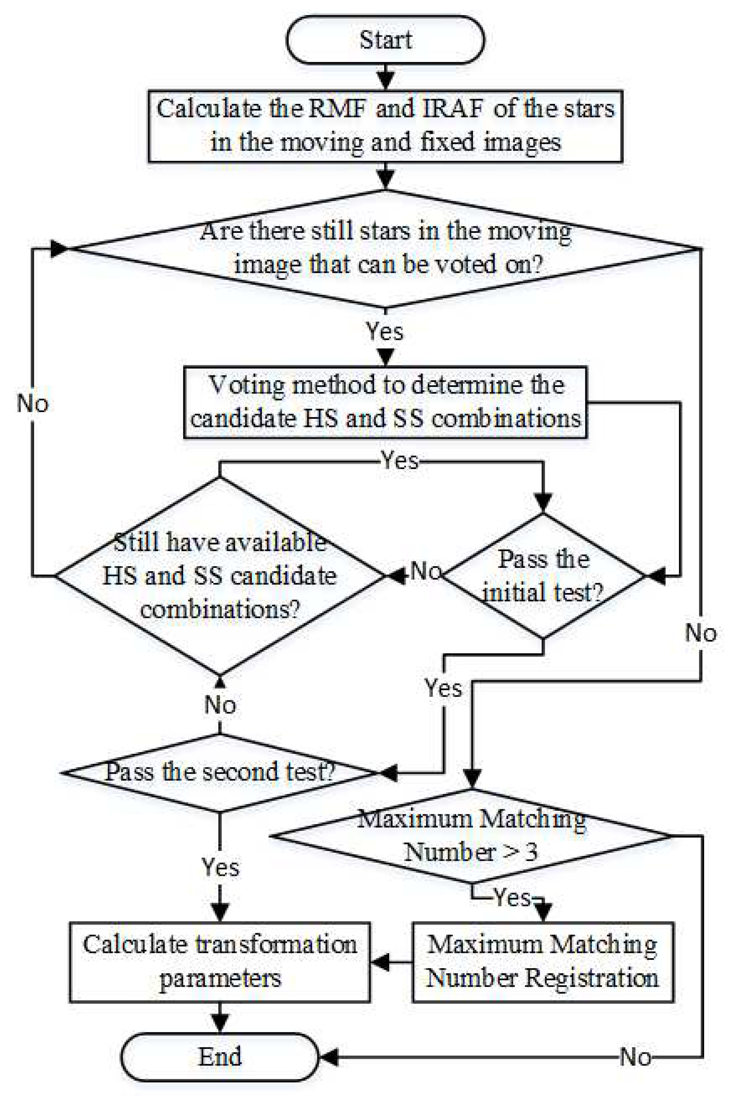
For easy understanding, the flow chart of the registration algorithm in this paper is given in
Figure 7.
4. Simulation and Real Data Testing
In this paper, the robustness, accuracy, and real-time of the algorithm are rigorously tested comprehensively from three perspectives: registration rate, registration accuracy, and running time using simulated and real data. It is also compared with the classical top-performing NCC [
14], FMT [
16], SURF [
20] and SPSG [
33,
34] registration algorithms. PC specifications: CPU: Montage Jintide(R) C6248R×4, RAM: 128GB, GPU: NVIDIA A100-40GB×4, where the GPU is mainly used to run the comparison algorithm SPSG.
4.1. Simulation Data Testing
The simulation parameters are field of view (FoV) 2.5 degrees, image size 1024*1024, detection capability (DC) 13Mv, 90% of the energy of the star image is concentrated in the area of 3*3, the maximum defocus blur diameter is 7 pixels, the length of the star image trailing is 15 pixels, and the trailing angle is 45 degrees. Image background is simulated using equation (
30).
where
x,
y denote the column and row coordinates of the pixel, respectively, and
is the parameter, which is set by statistics of 1000 real image backgrounds acquired at different times, and the specific values are shown in
Table 1. where
w is a random real variable with mean 0 and variance 1.
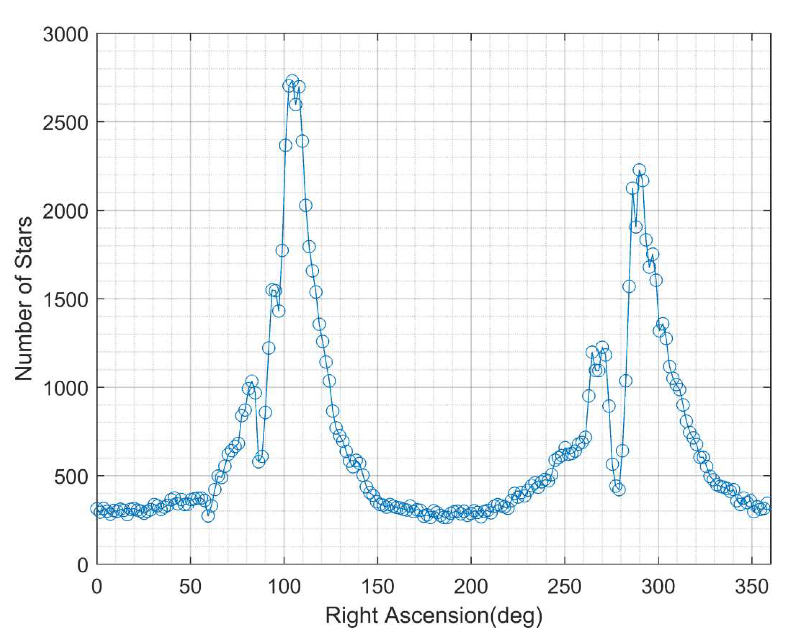
The ratio of high-frequency noise (speckle–shaped to simulate cosmic radiation noise and NEO objects) and hot pixels to total pixels, and the inter-image rotation angle are configured according to different test scenarios. The catalog used for the simulation is a union of Tycho–2, The third U.S. Naval Observatory CCD Astrograph Catalog (UCAC3) and Yale Bright Star Catalog 5th Edition (BSC5). The center of the field of view points to the Geostationary Orbit (GEO—an orbital belt with declination near 0 degrees and right ascension from 0 to 360 degrees), where the stellar density varies widely and the performance of the registration algorithm can be verified under different stellar density scenarios. The number of stars in the field of view corresponding to different right ascensions is shown in
Figure 8. Five scenarios of rotation, overlapping regions, false stars, position deviation and magnitude deviation, which are frequently encountered in star image registration, are tested using simulation data. The registration rate, registration accuracy and run time are calculated, where the registration rate refers to the ratio of the number of registered image pairs to the total number of pairs, the registration accuracy refers to the average distance between the matched reference stars after registration, the true value of the reference stars is provided in the image simulation, and the run time refers to the average run time of the registration algorithm. It should be noted that in the simulation, the positions of the stars are rounded, which causes a rounding error that follows a uniform distribution over the interval [-0.5,0.5], so if there is a rotation or translation between the simulated image pairs to be registered, there will be a registration error with a mean value of 0.52 pixels, as shown in equation (
31).
4.1.1. Rotation
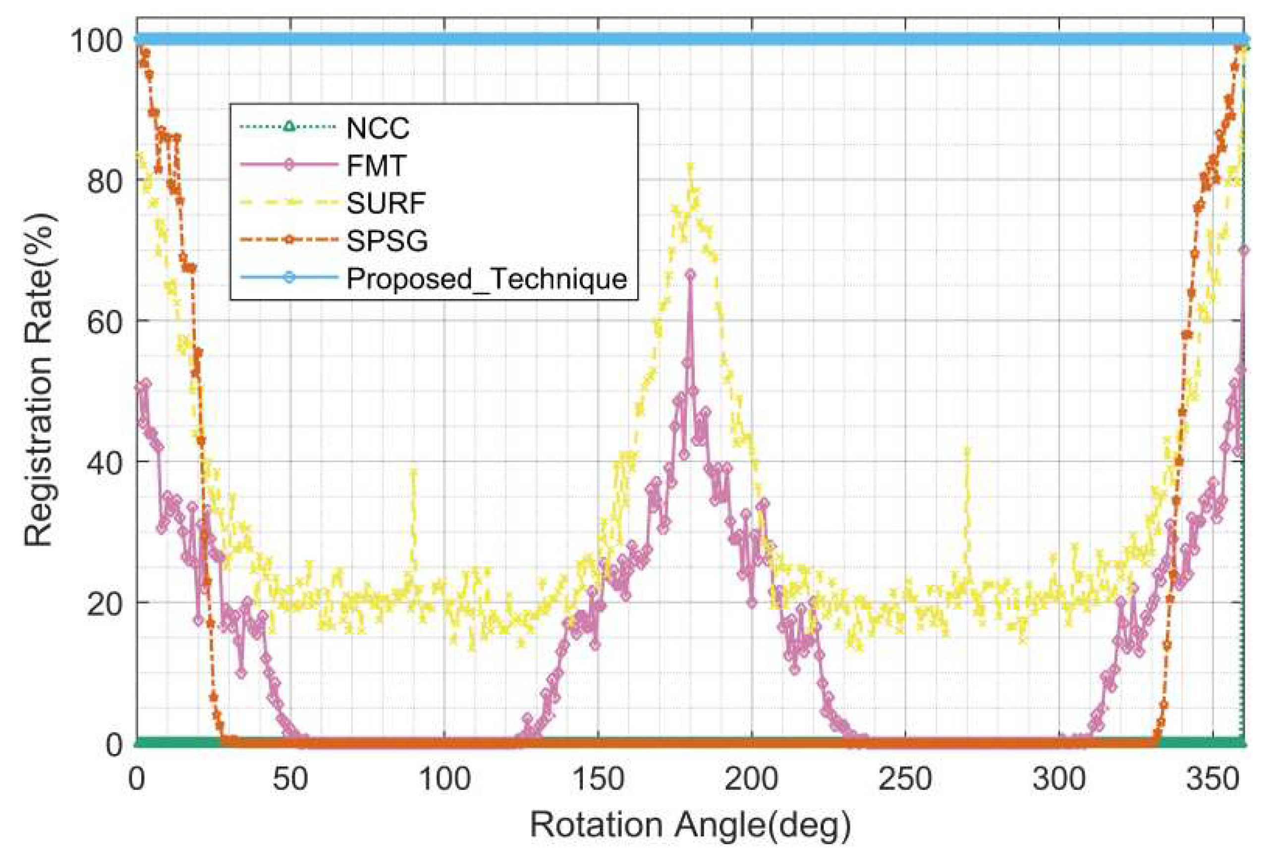
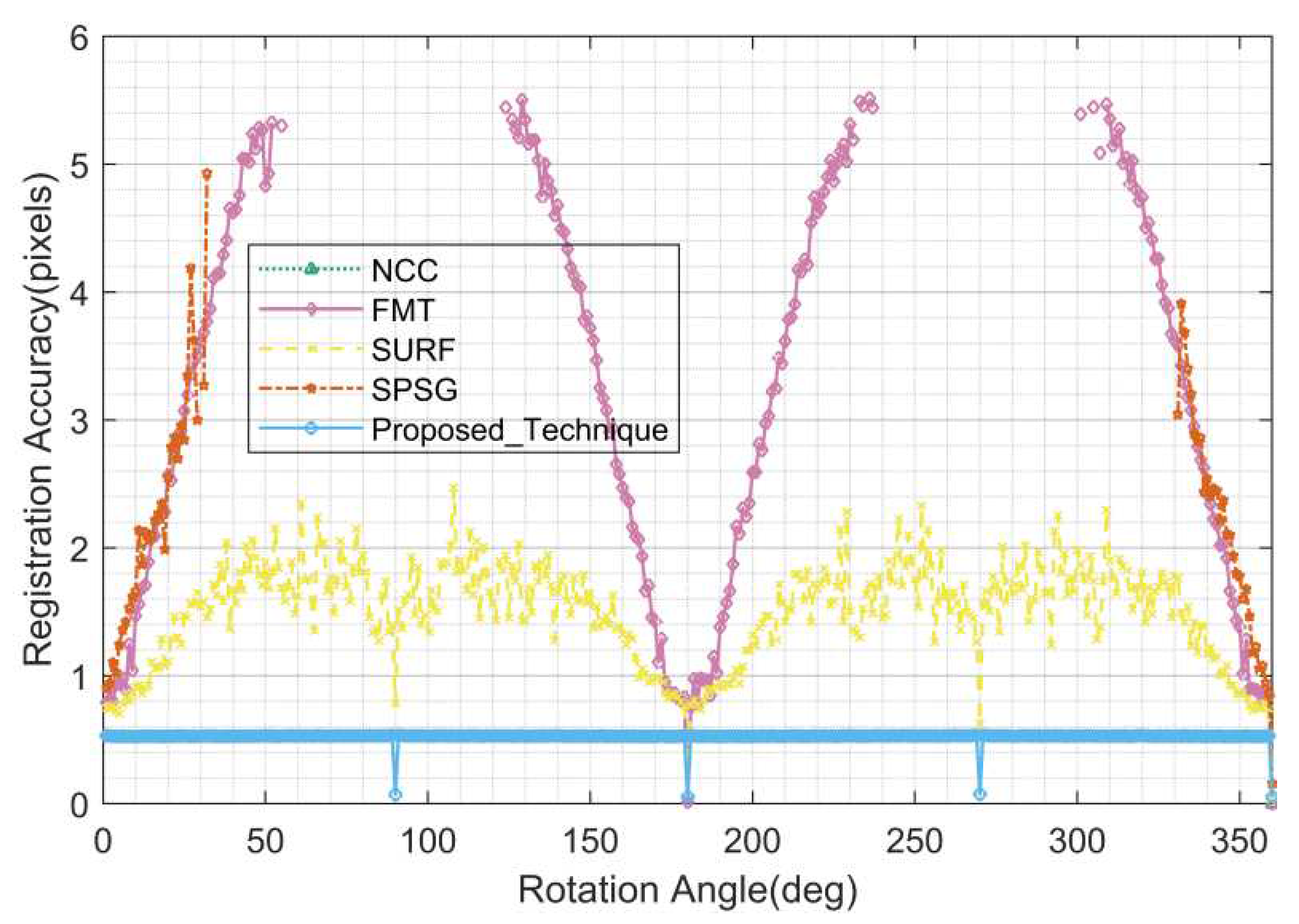
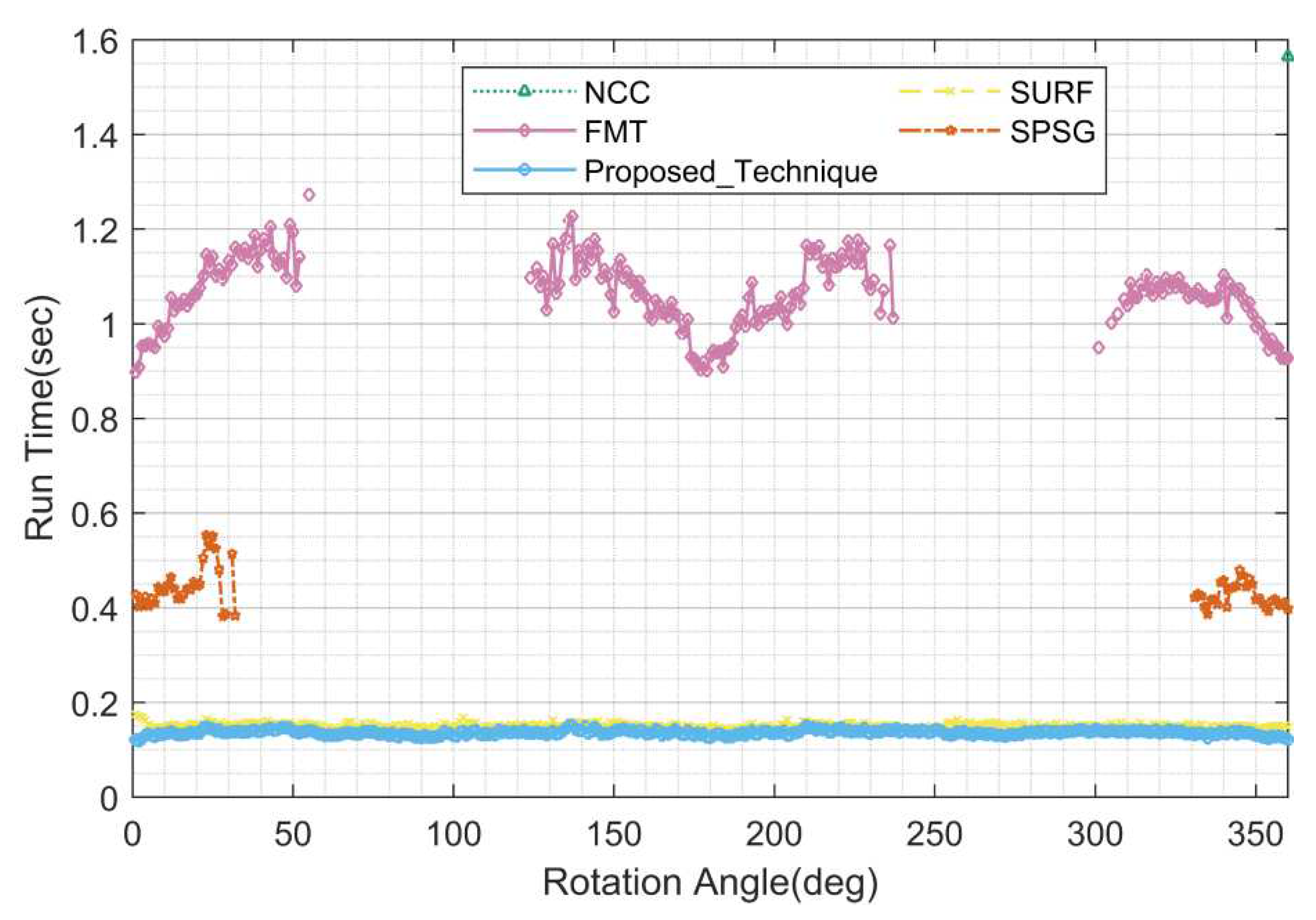
The purpose of this test is to test the performance of registration algorithms at different rotation angles between images. Specific configuration: rotation angle between images:1 to 360 degrees, step size: 1 degree; 200 pairs of images are tested for each rotation angle (center pointing: declination 0 degrees, right ascension: 0 to 358.2 degrees, step size: 1.8 degrees), total 72000 pairs of images; no high-frequency noise and hot pixels are added, the rest of parameters are default values.
Figure 9,
Figure 10, and
Figure 11 show the statistics of the registration rate, registration accuracy, and running time of each algorithm at different rotation angles in this test, respectively.
According to the statistical results, the performance of the proposed algorithm is completely unaffected by the rotation angle and is optimal. The registration rate is 100% for all rotation angles; the registration accuracy is about 0.5 pixels, which is mainly caused by the rounding error and the positioning error; the running time is about 0.15 seconds, which includes the running time of background suppression, star centroid extraction and registration, and the running time meets the requirement of real-time compared with the exposure time of several seconds or even ten seconds for star images. The registration performance of all compared algorithms in this test is poor, and only some of them are effective around 0 and 180 degrees, especially the grayscale based NCC algorithm completely invalidated due to its algorithm principle. It should be noted that the performance period of SURF and FMT algorithms is 180 degrees, while the performance period of SPSG algorithm is 360 degrees.
4.1.2. Overlapping regions
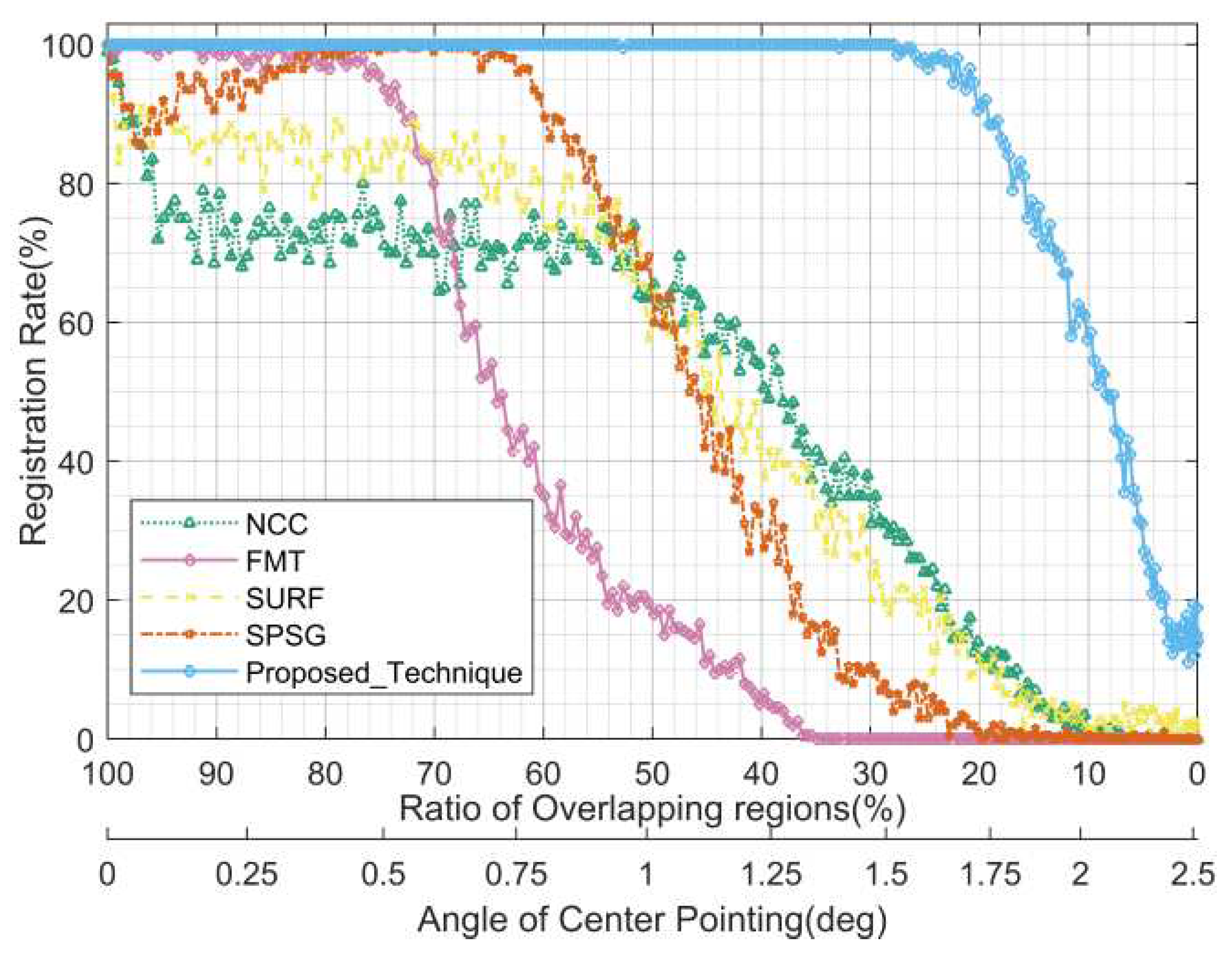
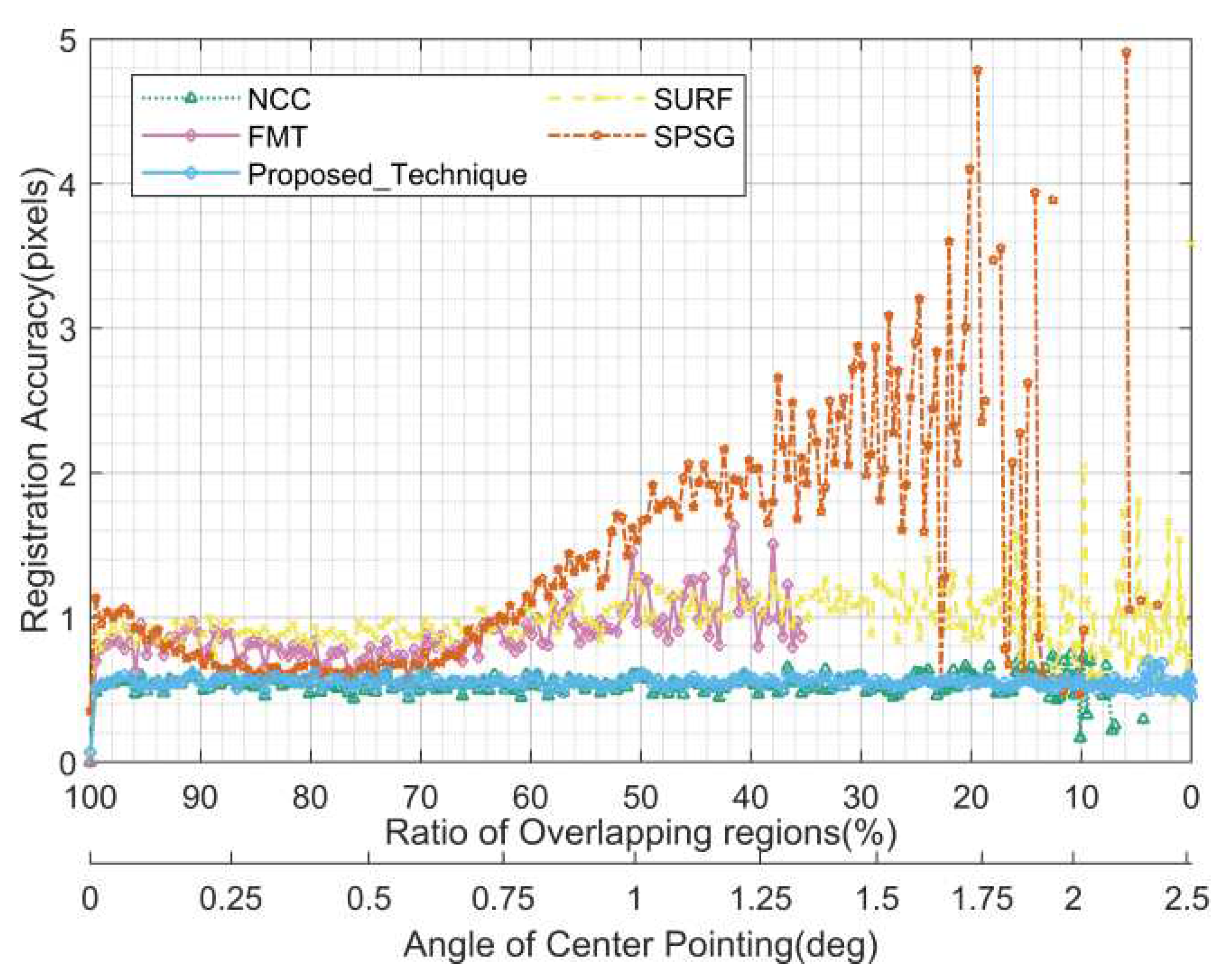
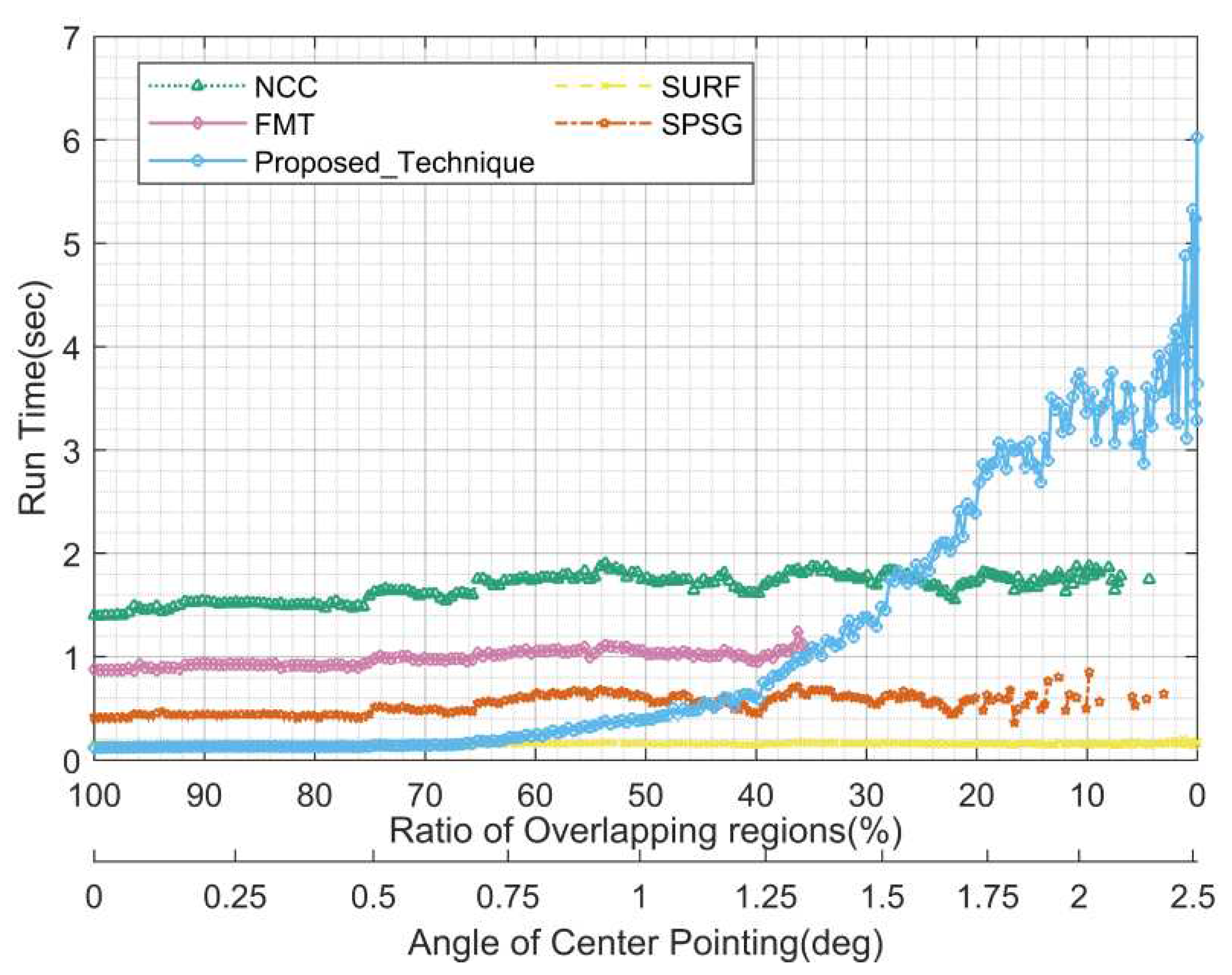
The purpose of this test is to test the performance of registration algorithms in different overlapping region between images. Specific configuration: angle between the center direction of the images to be registered: 0 to 2.5 degrees, step size: 0.01 degrees, corresponding to the percentage of the overlapping region in the image: 100% to 0; 200 pairs of images are tested for each angle (the right ascension and declination of the center of the fixed image are0 degrees; the centers of the moving images are uniformly distributed in concentric circle whose center is the center of the fixed image), total 50200 pairs of images; no high frequency noise and hot pixels added, no rotation between pairs of images, the rest of parameters are default values.
Figure 12,
Figure 13, and
Figure 14 show the statistics of the registration rate, registration accuracy, and running time for each algorithm at different overlapping regions in this test, respectively. Note that the overlap region here refers to the overlap region of the circular field of view, while the simulated image is square, so the actual overlap region will be larger, and even when the overlap region of the circular field of view is 0, there may still be a small overlap at the corners of the square field of view.
According to
Figure 12, the proposed algorithm is the most robust under different overlapping regions and can maintain 100% alignment rate when the proportion of overlapping regions is greater than 28% (the angle is less than 1.5 degrees), while the best performing NCC among the comparison algorithms in the same case is only about 30%. The FMT and SPSG algorithms outperform the NCC and SURF algorithms when the overlap region is large, while the latter two algorithms outperform the FMT and SPSG algorithms when the overlap region is small, which seems to be contrary to the previous experience that grayscale-based registration algorithms generally have lower registration rate than feature based registration algorithms when the overlap region is small. The registration accuracy of the proposed algorithm is maintained at about 0.5 pixels, which is also mainly caused by the rounding error and the positioning error; the registration accuracy of NCC is similar to that of the proposed algorithm, while the errors of the rest of the compared algorithms are slightly larger, especially the registration accuracy of the SPSG algorithm deteriorates sharply when the overlapping area is insufficient. In terms of running time, the proposed algorithm has a running time of about 0.15 seconds when the overlap region is larger than 60%, and then the running time gradually increases due to the increase of unmatched stars, and the running time is less than 1 second when the overlap region is larger than 34%, less than 3 seconds when the overlap region is larger than 14%, and no more than 6 seconds in the worst case. The real-time performance of the feature-based SURF and SPSG algorithms in the comparison algorithms is significantly better than the grayscale based FMT and NCC algorithms.
4.1.3. False stars
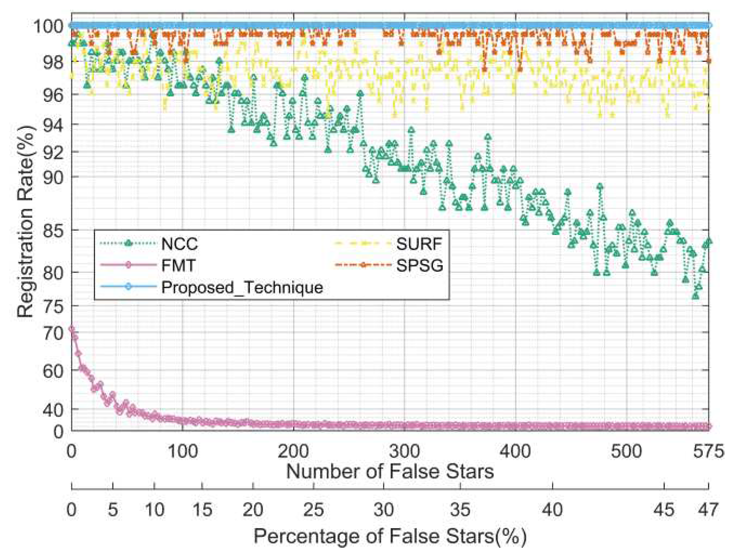
The purpose of this test is to test the performance of registration algorithms at different false stars densities. Here the false stars mainly refer to unmatched interference such as high frequency noise and hot pixels, which are simulated by adding speckle-like noise and highlighting single pixels. Specific configuration: speckle-like noise rate: 0 to 5e-04, step:2.5e-06, highlighted single pixels rate: 0 to 5e-05, step:2.5e-07, then total false stars rate: 0 to 5.5e-04, step:2.75e-06; each false stars rate is tested for 200 pairs of images (center pointing: declination 0 degrees, right ascension: 0 to 358.2 degrees, step size: 1.8 degrees), total 40200 image pairs; no rotation between image pairs, and the rest of parameters are default values.
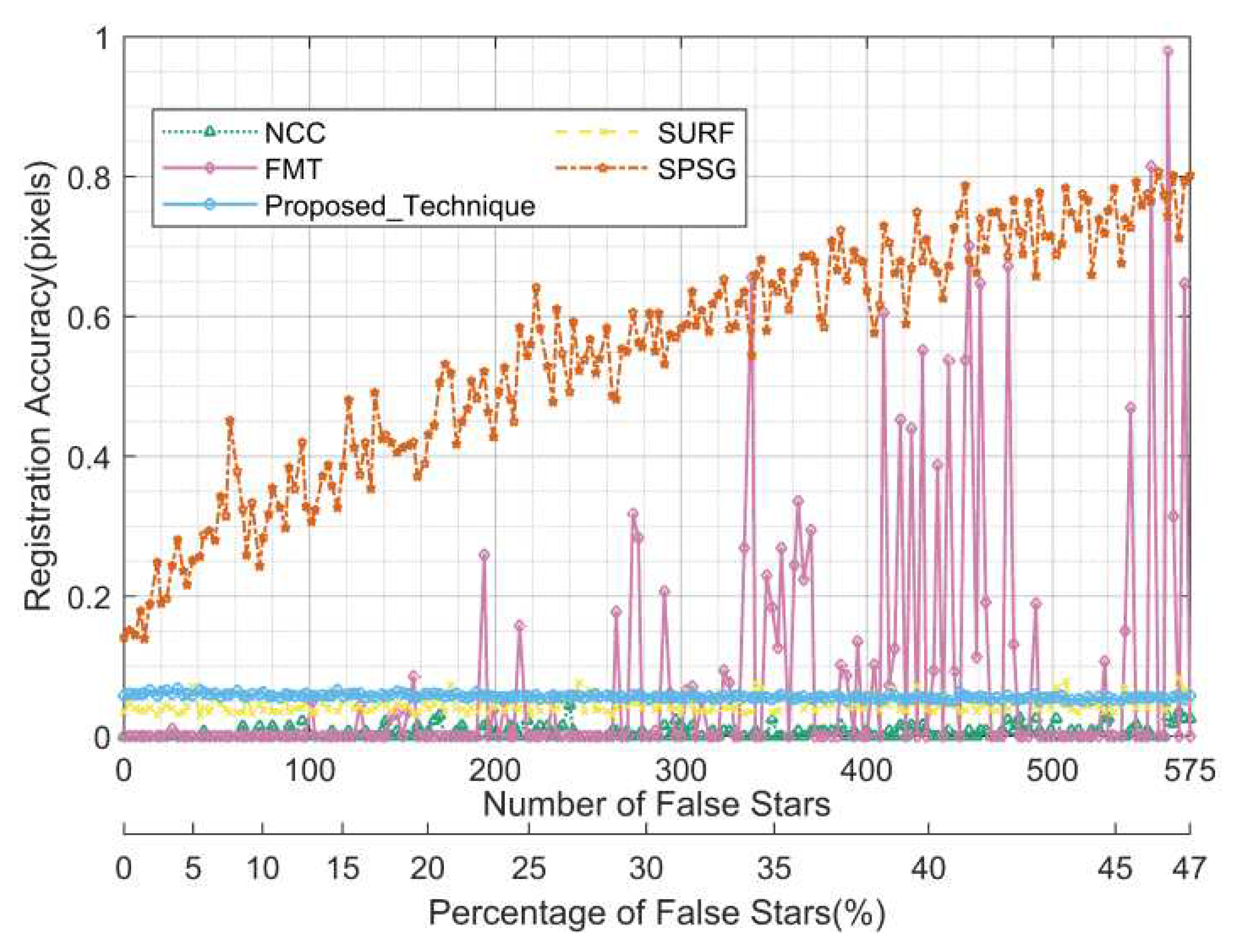
Figure 15,
Figure 16, and
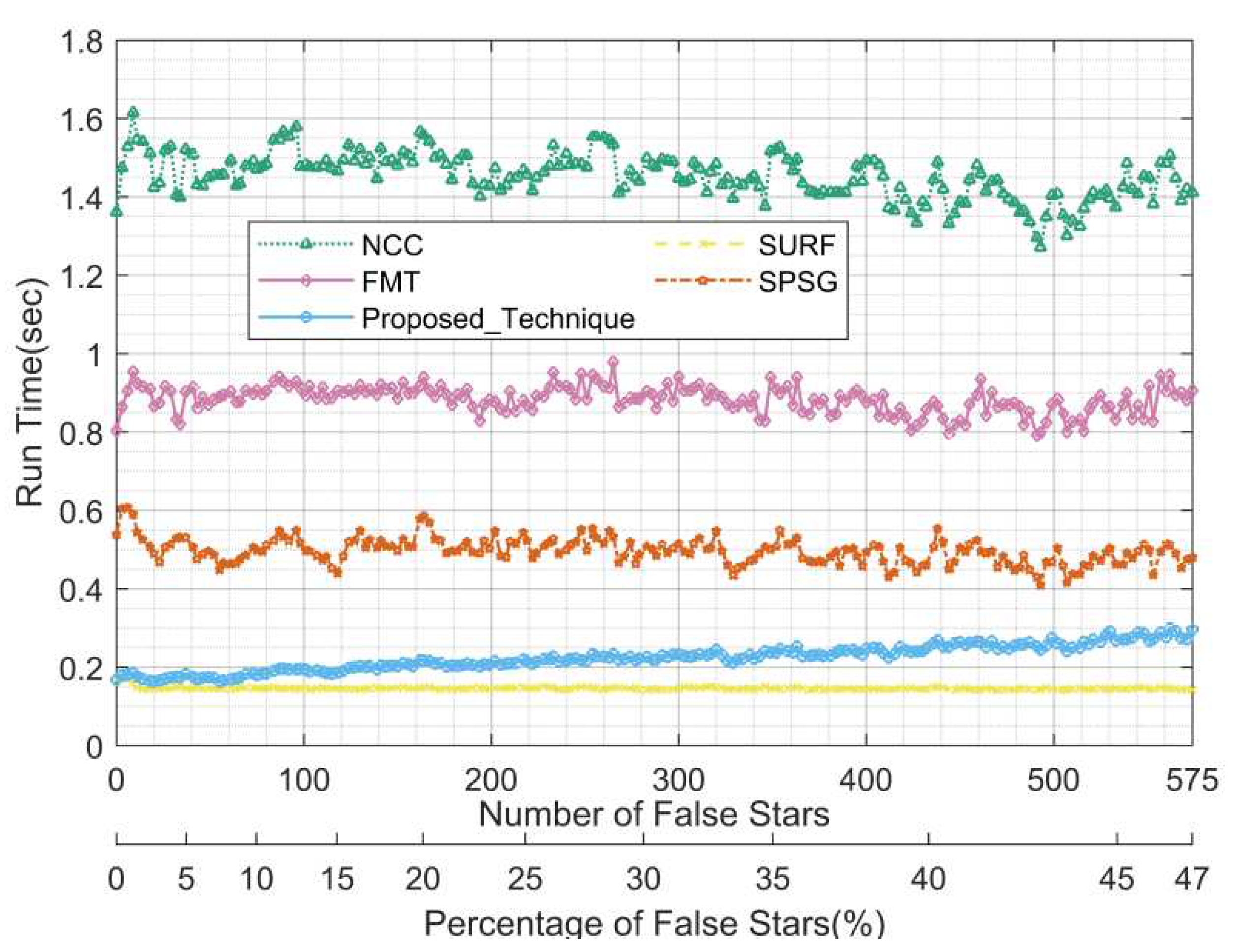
Figure 17 show the statistics of the registration rate, registration accuracy, and running time for each algorithm in this test for different numbers of false stars on the image (equivalent to the false stars rate) and different percentages of the number of false stars to the total number of object (the sum of the number of real stars and false stars), respectively.
As can be seen from
Figure 15, the proposed algorithm maintains the optimal registration rate of 100%, and the registration rates of the feature-based SPSG and SURF algorithms are significantly better than those of the grayscale-based NCC and FMT in the comparison algorithms, and are less affected by false stars, while the registration rates of the NCC and FMT algorithms are more affected by false stars, especially the FMT algorithm when there are more false stars, and the registration rate deteriorates sharply to near 0. As can be seen from
Figure 16, since there is no translation and rotation in this scene, it is not affected by the rounding error, so the registration accuracy is higher than 0.07 pixels for all the algorithms except for SPSG and FMT algorithms, which are slightly worse. As can be seen from
Figure 17, the overall feature-based algorithms are significantly better than grayscale-based algorithms in terms of run time. The run time of the proposed algorithm gradually increases from 0.15 to 0.3 seconds slightly inferior to the SURF algorithm, but fully satisfies the real-time requirement.
4.1.4. Position deviation
The purpose of this test is to test the performance of registration algorithms under different position deviations, and the process is simulated by adding Gaussian noise with a mean of 0 pixels and a standard deviation of
pixels to the row and column coordinates of the star, respectively. Specific configuration: 0
6, step size of 0.01 pixels, 200 pairs of images tested for each
value (center pointing: declination 0 degrees, right ascension: 0 to 358.2 degrees, step size: 1.8 degrees), 120200 pairs of images in total; no high frequency noise and hot pixels added, no rotation between pairs of images, the rest of parameters are default values.
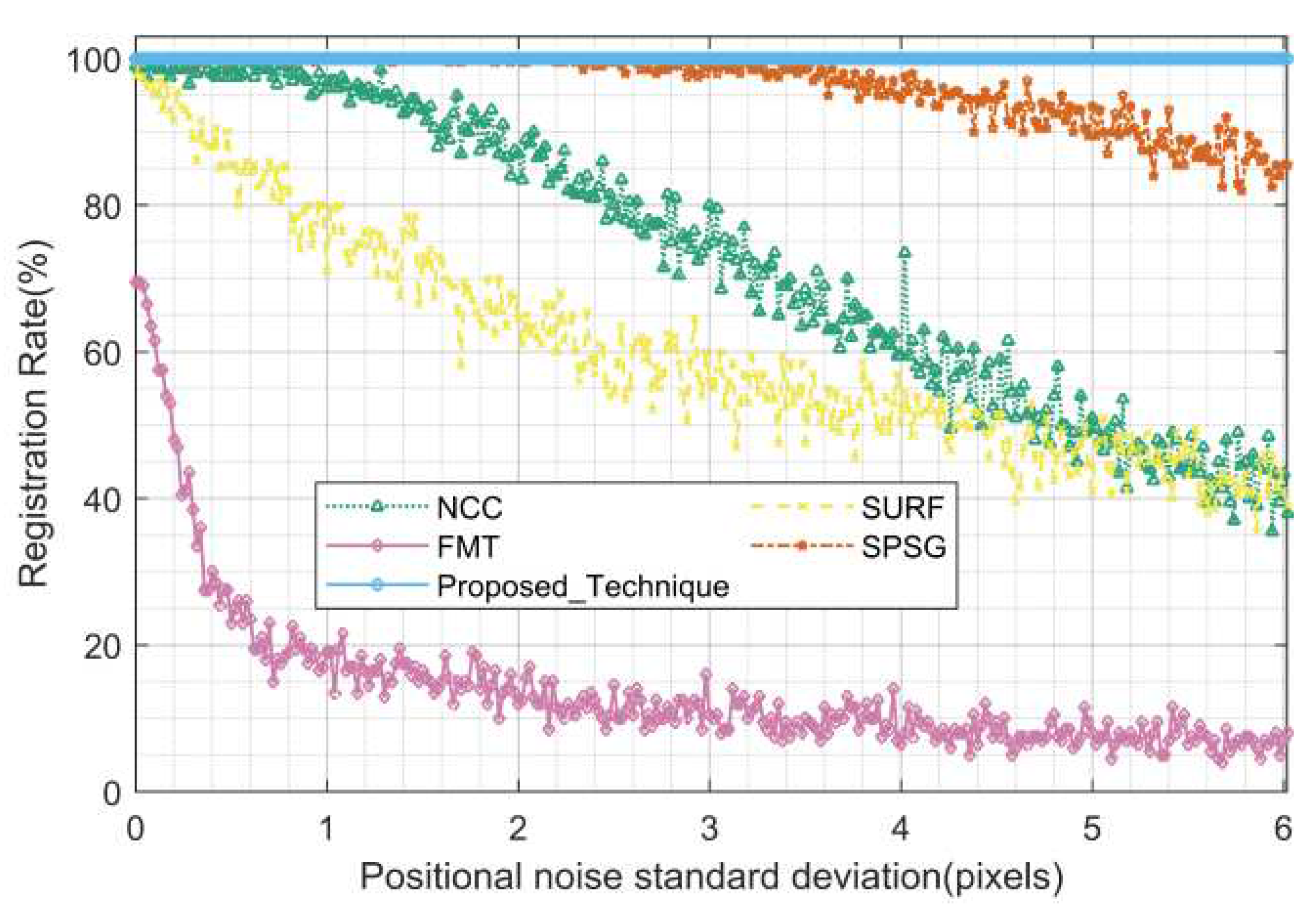
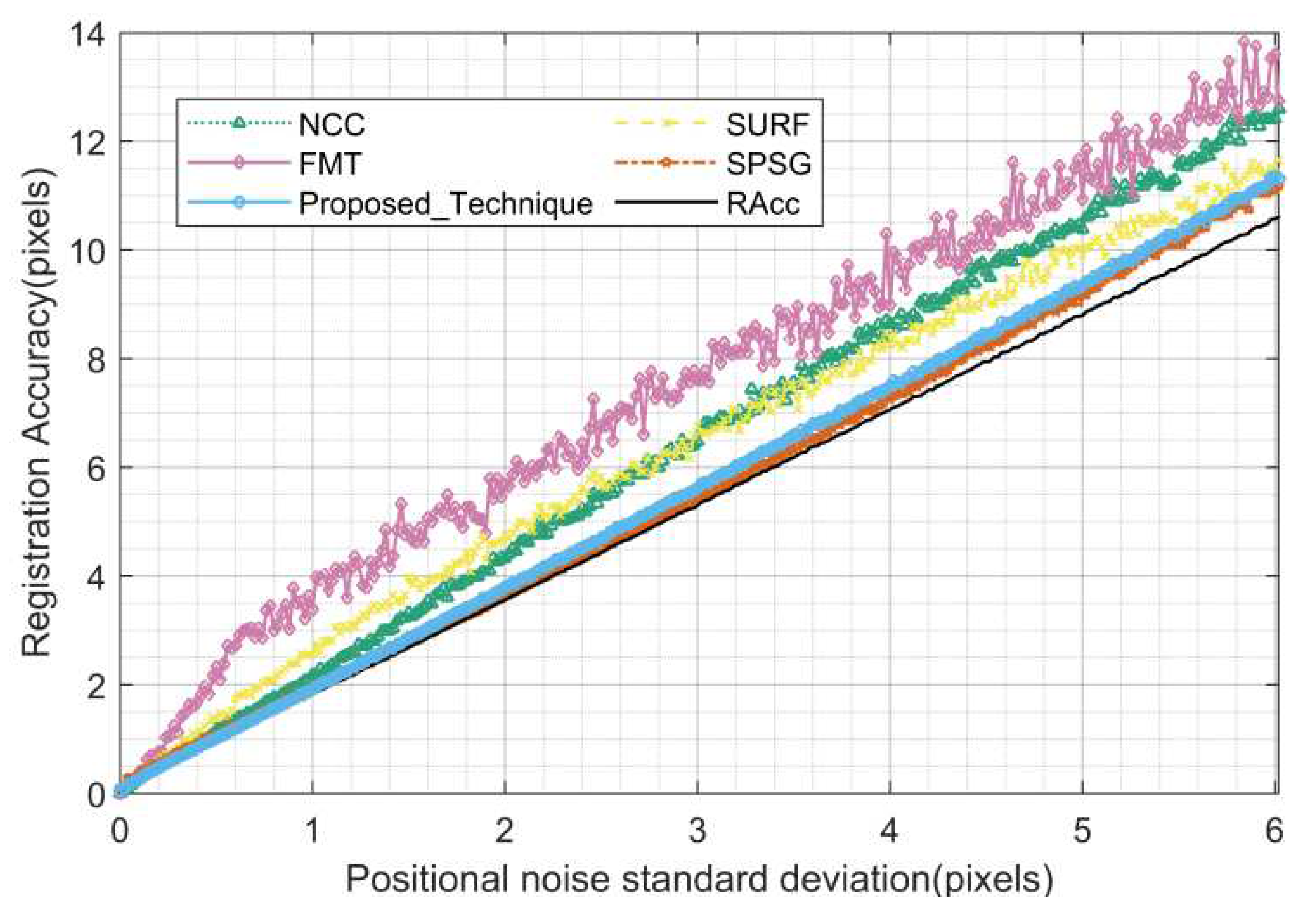
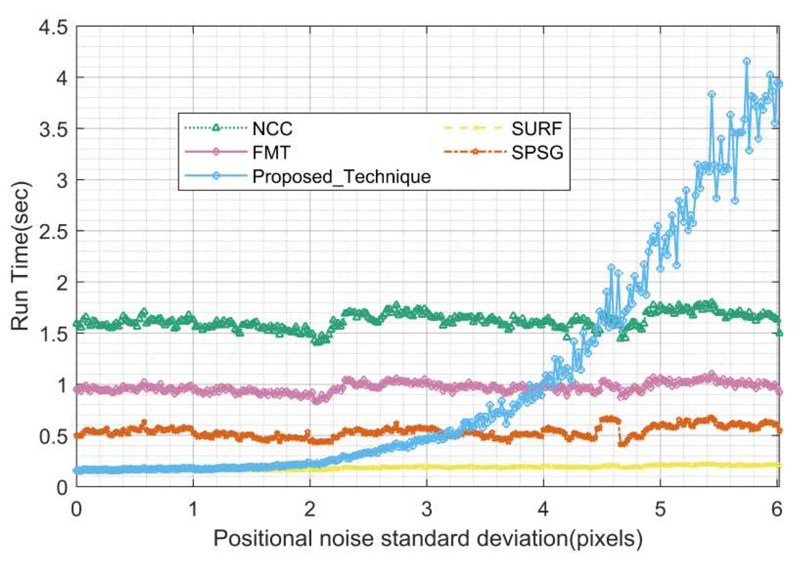
Figure 18,
Figure 19, and
Figure 20 show the statistics of the registration rate, registration accuracy and run time of each algorithm for different position deviations in this test, respectively.
As can be seen from
Figure 18, the proposed algorithm maintains the optimal registration rate of 100%, in comparative algorithms, the SPSG has a better registration rate of more than 80%, the FMT is the worst, and slightly surprisingly, the NCC has a better registration rate than the SURF. For the registration accuracy, the reference accuracy calculated based on the real simulation coordinates (”Racc” in
Figure 19, black solid line) was added to the statistics as a comparison because of the preset position deviation during the simulation of this scene. As can be seen from
Figure 19, in terms of registration accuracy, the proposed algorithm and SPSG are the best, with little difference from the reference accuracy, the FMT is the worst, and the NCC and SURF have about the same registration accuracy. As can be seen from
Figure 20, in terms of run time, all the compared algorithms are relatively smooth, and the feature-based SURF and SPSG algorithms are better than the grayscale-based NCC and FMT algorithms, and the proposed algorithms are comparable to the SURF in about0.15 seconds when the position deviation is less than 2 pixels, and the run time gradually increases to about 4 seconds when the deviation is greater than 2 pixels because the combination of the HS and the SS needs to be verified several times.
4.1.5. Magnitude deviation
The purpose of this test is to test the performance of registration algorithms with different magnitude deviations, simulating the process by adding Gaussian noise with a mean of 0 Mv and a standard deviation of
Mv to the real magnitude values. Specific configuration: 0
2 with a step size of 0.01 Mv; 200 pairs of images were tested for each
value (center pointing: declination 0 degrees, right ascension: 0 to 358.2 degrees, step size: 1.8 degrees), 40200 pairs of images in total; no high-frequency noise and hot pixels were added, no rotation between image pairs, and the remaining parameters were default values.
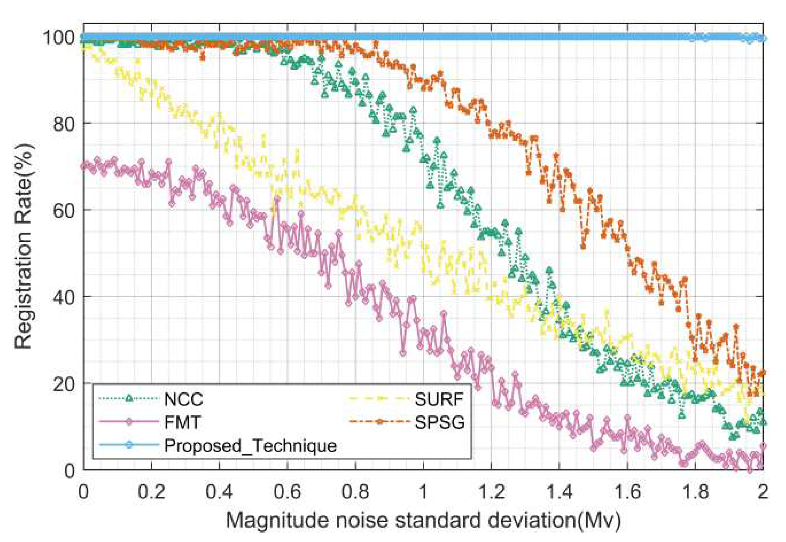
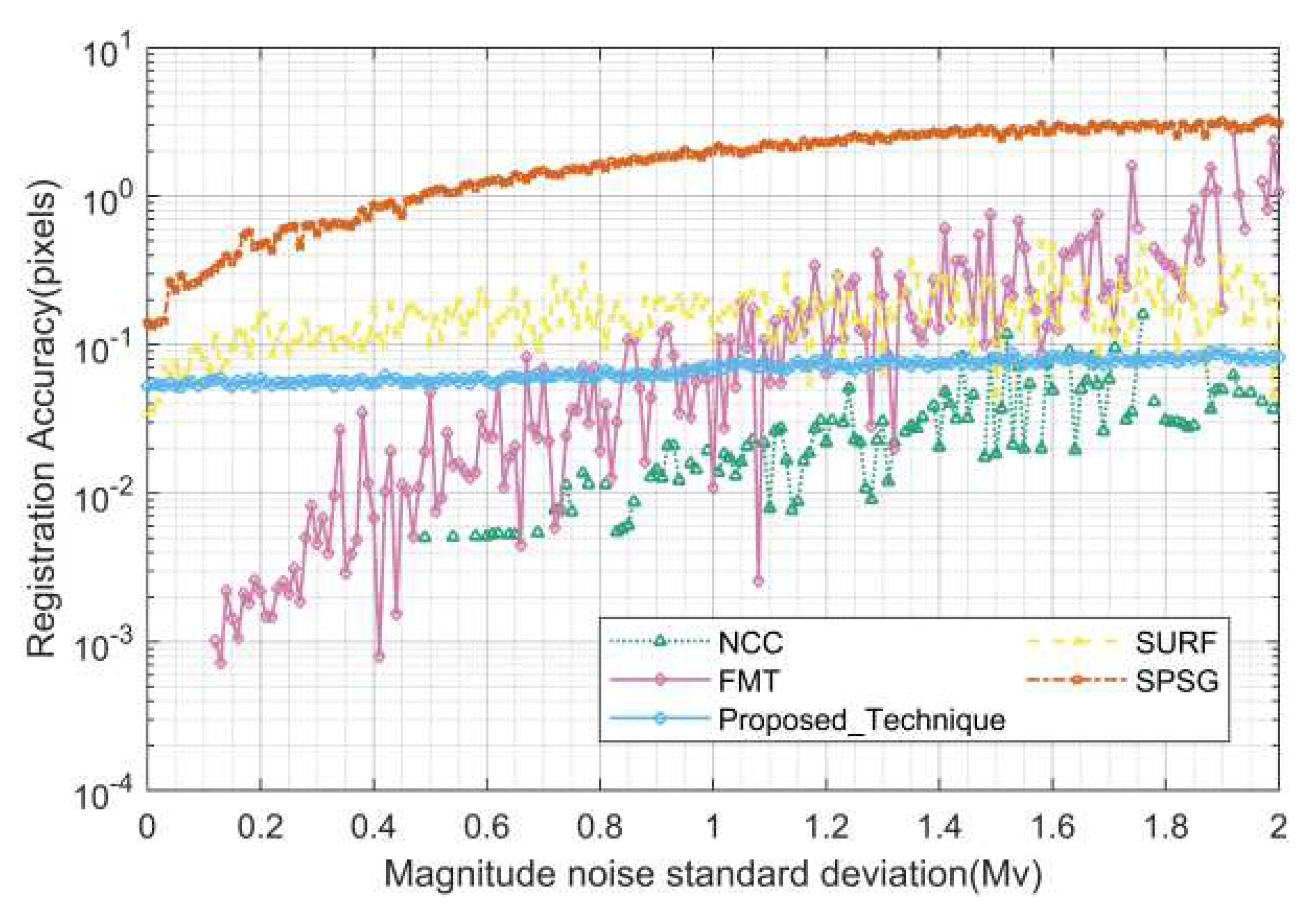
Figure 21,
Figure 22, and
Figure 23 show the statistics of the registration rate, registration accuracy, and run time of each algorithm for different magnitude deviations in this test, respectively.
As can be seen from
Figure 21, in terms of the registration rate, the proposed algorithm maintains the optimal registration rate of 100%, in comparison algorithms, the SPSG algorithm performs better, the FMT algorithm is the worst, and the NCC algorithm has a better registration rate than the SURF algorithm, which also seems to be contrary to the previous experience that the grayscale–based registration is inferior to the feature-based registration algorithm when there is a deviation in magnitude (or brightness). As can be seen from
Figure 22, the registration accuracy is high for all the algorithms except SPSG because the scene has no translation and rotation, so it is not affected by the rounding error. The registration accuracy of the proposed algorithms ranges from 0.05 to 0.1 pixel, NCC and SURF fluctuate slightly, and SPSG gradually deteriorates to 3.5 pixels when the magnitude deviation is greater than 0.5 Mv. As can be seen from
Figure 23, in terms of run time, all compared algorithms are basically the same as in other test scenarios. The proposed algorithm is optimal with run time less than 0.2 seconds when the magnitude deviation is less than 1.6 Mv, and the run time increases gradually with magnitude deviation greater than 1.6 Mv but the maximum time does not exceed 0.7 seconds.
4.2. Real Data Testing
Real data parameters: field of view 2.5 degrees, image size 1024*1024, detection capability about 13 Mv; including a total of 338577 real star images in 523 tasks over 31 days. The more complex imaging environment of the real data can better test the comprehensive performance of algorithms, especially the real complex background simulation algorithm is difficult to simulate realistically, so the real images can well test the algorithm’s registration performance of star images in complex backgrounds. Similar to the simulation data, the three indexes of registration rate, registration accuracy and run time are also counted in the test using the real data. The difference is that the true value of the reference point cannot be provided in the calculation of the registration accuracy as in the simulation data, and the result of the algorithm with the largest number of matched star pairs among all algorithms is selected here as a reference. It should be noted that due to the limitations of the telescope operation mode, there is no rotation between all real images here, but the performance of the algorithms in the presence of image rotation has been adequately tested in the simulation data testing.
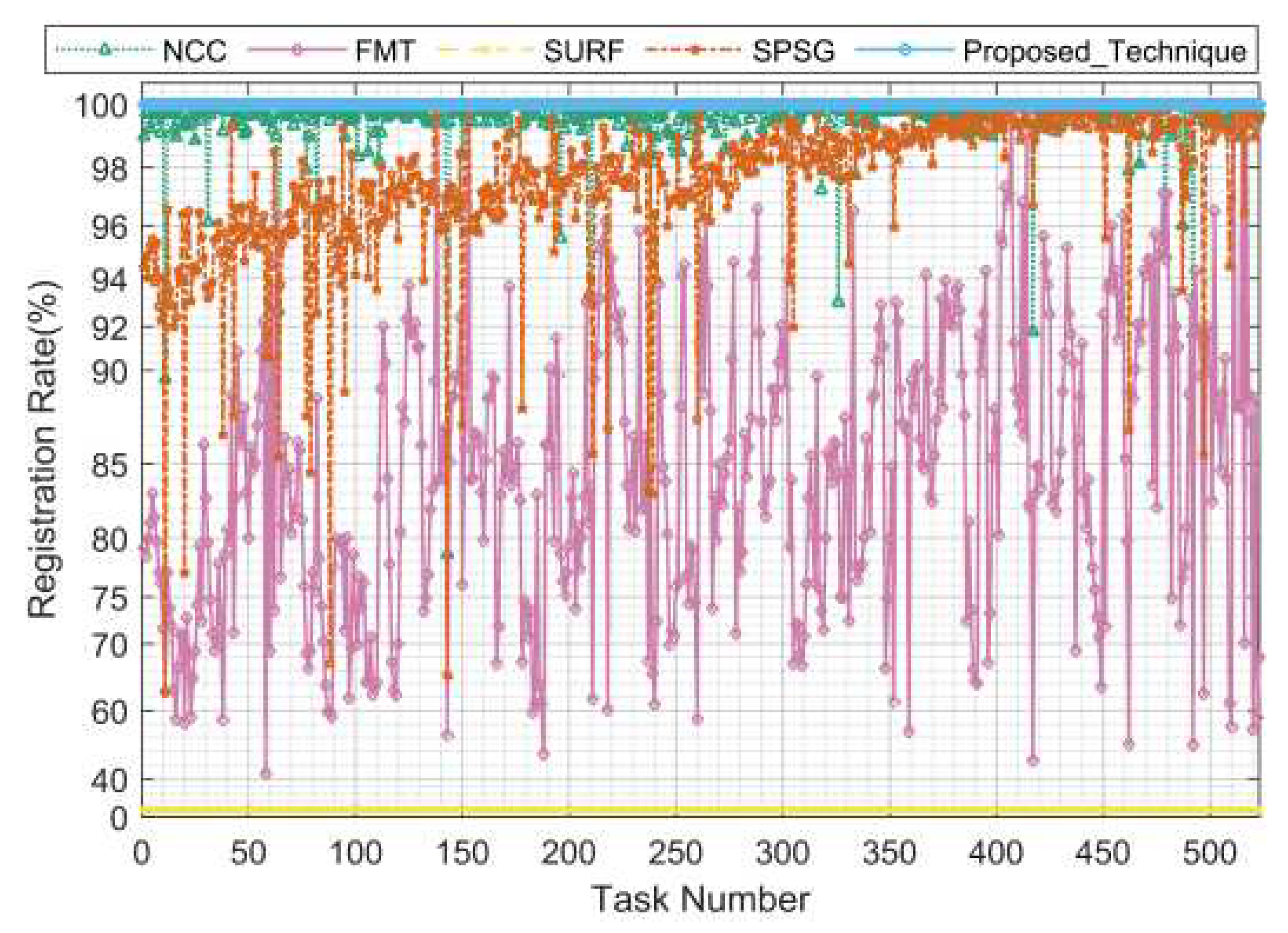
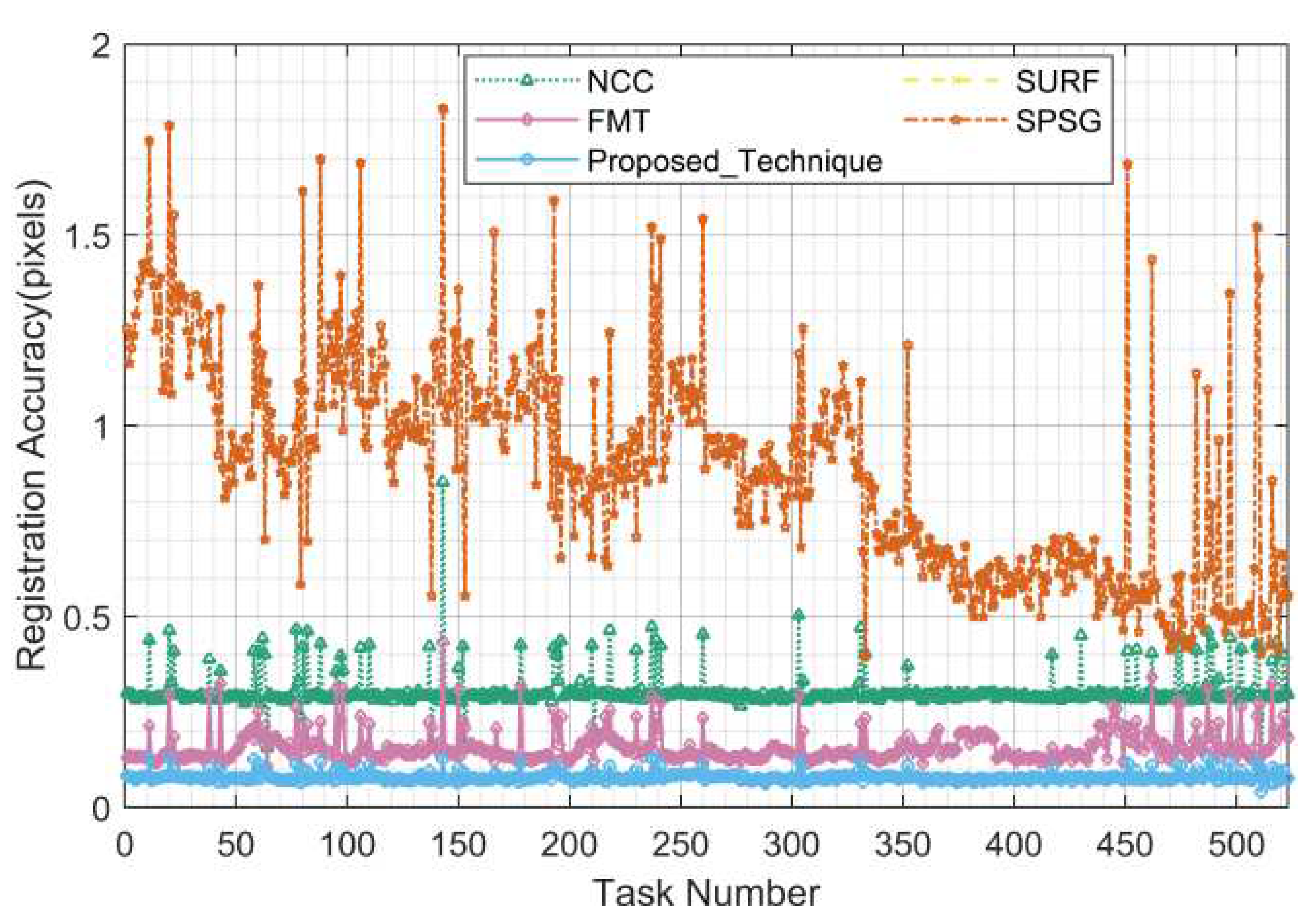
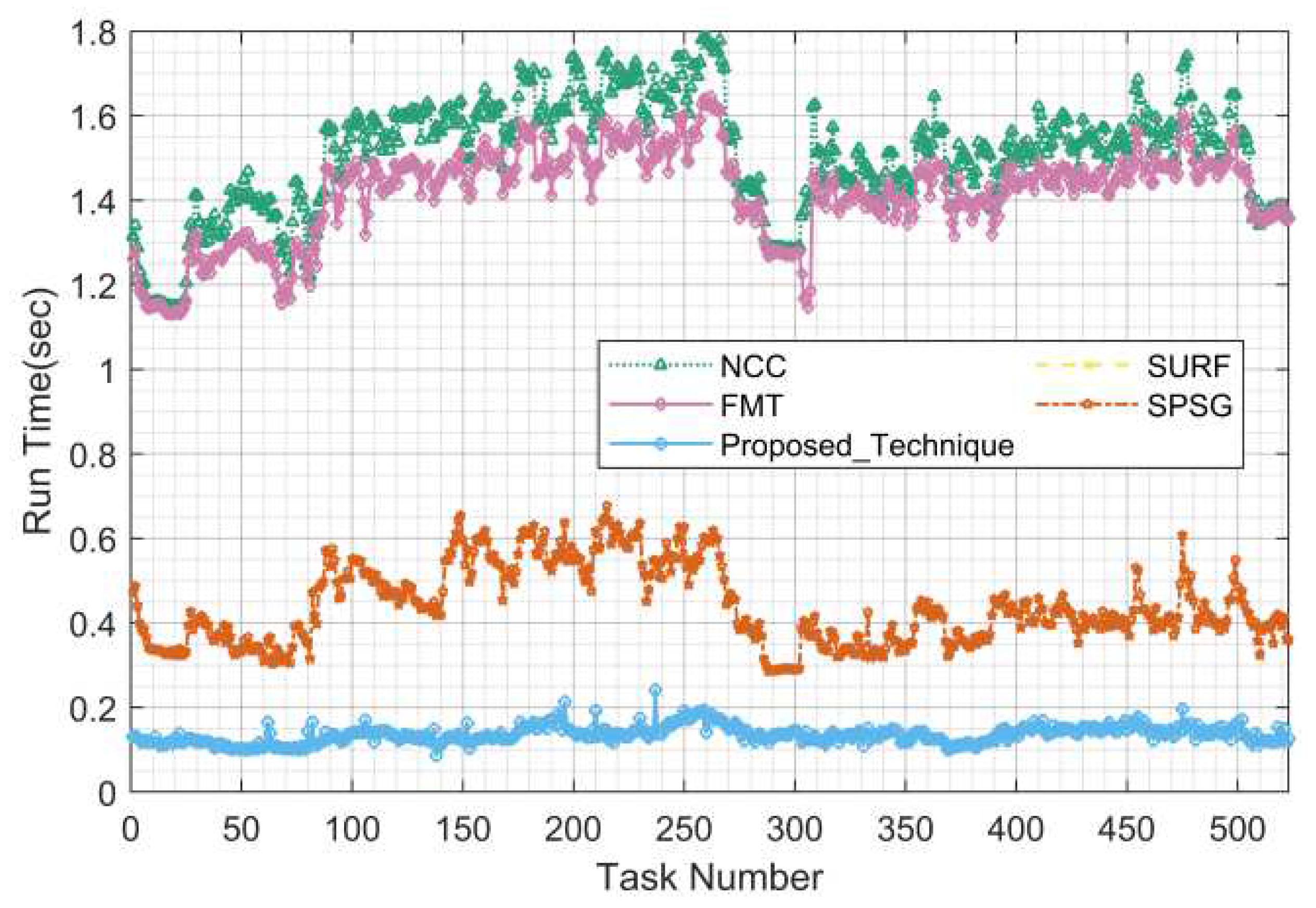
Figure 24,
Figure 25, and
Figure 26 show the statistics of the registration rate, registration accuracy, and run time of each algorithm under different tasks, respectively.
According to the statistical results, the proposed algorithm is optimal in terms of registration rate, registration accuracy and running time; the biggest unexpected is that the SURF algorithm is completely ineffective in the registration of real star images, probably because it cannot adapt to the complex background of real star images. As can be seen in
Figure 24, in terms of the registration rate, the proposed algorithm maintains 100% registration rate, in the comparison algorithms, the NCC algorithm achieves more than 98% registration rate in most of the tasks, the SPSG algorithm fluctuates slightly but is able to achieve more than 92% in most of the tasks, the FMT algorithm’s registration rate fluctuates greatly between 40% and 100%, and the SURF is completely ineffective. As can be seen from
Figure 25, in terms of registration accuracy, the proposed algorithm has the best performance, with a registration accuracy of about 0.1 pixels for all tasks, since there is no rounding error in the real data and therefore the error is mainly caused by positioning errors; the accuracy of the FMT algorithm is between 0.15 and 0.2 pixels for most tasks; the accuracy of the NCC algorithm is between 0.3 and 0.5 pixels, mostly around 0.3; The SPSG algorithm registration accuracy is poor between 0.4 and 1.85 pixels. As can be seen from
Figure 26, in terms of run time, the proposed algorithm is optimal at around 0.15 seconds; the SPSG algorithm is second between 0.3 and 0.7 seconds; the grayscale based NCC and FMT algorithms have the longest run time between 1.1 and 1.8 seconds.
5. Discussion
This section discusses the comprehensive performance of star image registration algorithms.In order to obtain the comprehensive performance scores of the proposed algorithm and the compared algorithms, the following is a comprehensive evaluation of each algorithm based on the registration rate, registration accuracy and run time of each algorithm in processing simulated images with rotation, overlapping area change, false stars, position deviation, magnitude deviation and real images. In this paper, we use the scoring strategy as shown in equation (
32).
Where
N is the number of registered image pairs,
,
and
are the scores of the
pair of registration success rate, registration accuracy and run time, respectively, and
and
are the weights of registration accuracy and run time, respectively. Considering that in practice, the registration accuracy can better reflect the core performance of the algorithm compared with the run time, and the run time can be improved by parallel design or upgrading the hardware performance and increasing the number of hardware, therefore, the weight of registration accuracy is greater here. The specific definitions of
,
and
are as follows.
where,
is the registration accuracy of the registration algorithm and
is the reference accuracy.
where,
is the run time of the registration algorithm.
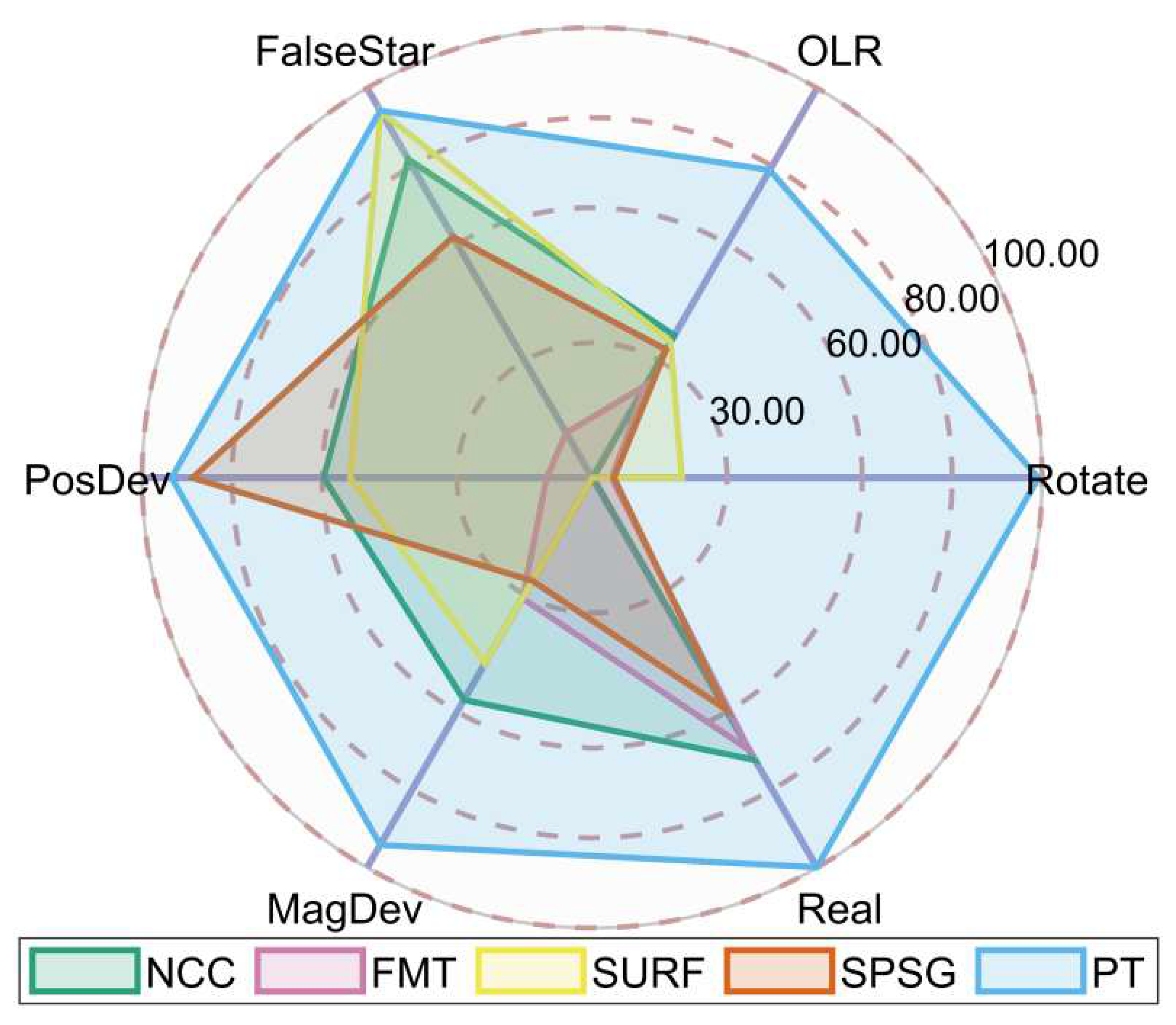
Table 2 shows the statistics of the comprehensive performance of the algorithms, where ”OLR” represents the overlapping region test, ”PT” represents the algorithm proposed in this paper, and ”Score” is the average score of all test items to evaluate the comprehensive performance of the algorithms. Star image registration algorithms comprehensive performance radar chart is shown in
Figure 27.
From
Table 2 and
Figure 27, it can be seen that the comprehensive performance of the proposed algorithm is significantly better than all the comparison algorithms in all scenes, and the performance is more balanced, and only slightly worse in the overlapping region change test. All comparison algorithms have poor processing performance in the presence of rotation and insufficient overlapping region between images. The NCC algorithm performs better in processing images with false stars and real images without rotation. Although the FMT algorithm does not perform well when processing simulated images, it performs reasonably well when processing real images without rotation by virtue of its high registration accuracy. The SURF algorithm performs better in processing images with false stars, but it cannot register real images, probably because it cannot adapt to complex real backgrounds, so to register real star images with SURF it must be used with a high-performance background suppression algorithm. The SPSG algorithm performs reasonably well in processing images with false stars and position deviations.
6. Conclusions
In this paper, we propose a registration algorithm for star images, which relies only on RMF and RAF. The test results using a large amount of simulated and real data show that the comprehensive performance of the proposed algorithm is significantly better than the comparison algorithms when there are rotation, insufficient overlapping region, false stars, position deviation, magnitude deviation and complex sky background, and it is a more ideal star image registration algorithm. The test results also show that the proposed algorithm has a longer running time when the overlap region is too small or the position deviation is too large, which can be improved in the future work. In addition, the robustness, real-time performance and registration accuracy of the current classical registration algorithms of NCC, FMT, SURF and SPSG in the field of star image registration are fully tested in this paper to provide valuable references for future related researches or applications.
Author Contributions
Conceptualization, S.Q.; methodology, S.Q.; software, S.Q.; validation, S.Q. , L.L. and Z. J.; formal analysis, S.Q.; investigation, S.Q.; resources, N.Z.; data curation, L.Y.; writing—original draft preparation, S.Q.; writing—review and editing, N.Z. and W.Z.; visualization, S.Q.; supervision, N.Z.; project administration, N.Z.; funding acquisition, N.Z. All authors have read and agreed to the published version of the manuscript.
Funding
This research was funded in part by the Youth Science Foundation of China (Grant No.61605243).
Data Availability Statement
The simulation data supporting the results of this study are available from the corresponding author upon reasonable request. The raw real image data is cleaned periodically due to its excessive volume, but intermediate processing results are available upon reasonable request.
Acknowledgments
The authors thank the Xi’an Satellite Control Center for providing real data to fully validate the performance of the algorithm, and are also very grateful to all the editors and reviewers for their hard work on this paper.
Conflicts of Interest
The authors declare no conflict of interest.
References
- Jiang, P.; Liu, C.; Yang, W.; Kang, Z.; Fan, C.; Li, Z. Automatic extraction channel of space debris based on wide-field surveillance system. npj Microgravity 2022, p. 14. [CrossRef]
- Barentine, J.C.; Venkatesan, A.; Heim, J.; Lowenthal, J.; Kocifaj, M.; Bará, S. Aggregate effects of proliferating low-Earth-orbit objects and implications for astronomical data lost in the noise. Nature Astronomy 2023, pp. 252–258. [CrossRef]
- Li, Y.; Niu, Z.; Sun, Q.; Xiao, H.; Li, H. BSC-Net: Background Suppression Algorithm for Stray Lights in Star Images. Remote Sensing 2022, 14. [Google Scholar] [CrossRef]
- Li, H.; Niu, Z.; Sun, Q.; Li, Y. Co-Correcting: Combat Noisy Labels in Space Debris Detection. Remote Sensing 2022, 14. [Google Scholar] [CrossRef]
- Liu, L.; Niu, Z.; Li, Y.; Sun, Q. Multi-Level Convolutional Network for Ground-Based Star Image Enhancement. Remote Sensing 2023, 15. [Google Scholar] [CrossRef]
- Shou-cun, H.; Hai-bin, Z.; Jiang-hui, J. Statistical Analysis on the Number of Discoveries and Discovery Scenarios of Near-Earth Asteroids. Chinese Astronomy and Astrophysics 2023, pp. 147–176. [CrossRef]
- Ivezic, Z (Ivezic, Z.; Kahn, SM (Kahn, S.M.; Tyson, JA (Tyson, J.A.; Abel, B (Abel, B.; Acosta, E (Acosta, E.; Allsman, R (Allsman, R.; Alonso, D (Alonso, D.; AlSayyad, Y (AlSayyad, Y.; Anderson, SF (Anderson, S.F.; Andrew, J (Andrew, J. LSST: From Science Drivers to Reference Design and Anticipated Data Products. Astrophys.J. 2019, p. 111.
- Bosch, J.; AlSayyad, Y.; Armstrong, R.; Bellm, E.; Chiang, H.F.; Eggl, S.; Findeisen, K.; Fisher-Levine, M.; Guy, L.P.; Guyonnet, A.; et al. An Overview of the LSST Image Processing Pipelines. Astrophysics 2018.
- Mong, Y.L.; Ackley, K.; Killestein, T.L.; Galloway, D.K.; Vassallo, C.; Dyer, M.; Cutter, R.; Brown, M.J.I.; Lyman, J.; Ulaczyk, K.; et al. Self-supervised clustering on image-subtracted data with deep-embedded self-organizing map. Monthly Notices of the Royal Astronomical Society 2023, pp. 752–762. [CrossRef]
- Singhal, A.; Bhalerao, V.; Mahabal, A.A.; Vaghmare, K.; Jagade, S.; Kulkarni, S.; Vibhute, A.; Kembhavi, A.K.; Drake, A.J.; Djorgovski, S.G.; et al. Deep co-added sky from Catalina Sky Survey images. Monthly Notices of the Royal Astronomical Society 2021, pp. 4983–4996.
- Yu, C (Yu, C.; Li, BY (Li, B.; Xiao, J (Xiao, J.; Sun, C (Sun, C.; Tang, SJ (Tang, S.; Bi, CK (Bi, C.; Cui, CZ (Cui, C.; Fan, DW (Fan, D. Astronomical data fusion: Recent progress and future prospects — a survey(Review). Experimental Astronomy 2019, pp. 359–380.
- Paul, S.; Pati, U.C. A comprehensive review on remote sensing image registration. International Journal of Remote Sensing 2021, pp. 5400–5436. [CrossRef]
- Wu, Peng, w.; Li, W.; Song, W.; Balas, V.E.; Hong, J.L.; Gu, J.; Lin, T.C. Fast, accurate normalized cross-correlation image matching. Journal of Intelligent & Fuzzy Systems 2019, pp. 4431–4436.
- Lewis, J. Fast Normalized Cross-Correlation. Vision Interface 1995, pp. 120–123.
- Yan, X.; Zhang, Y.; Zhang, D.; Hou, N.; Zhang, B. Registration of Multimodal Remote Sensing Images Using Transfer Optimization. IEEE Geoscience and Remote Sensing Letters 2020, pp. 2060–2064. [CrossRef]
- S., R.B. A FFT - Based Technique for Translation, Rotation and Scale - Invariant Image Registration. IEEE Transaction on Image Processing 1996, pp. 1266–1271.
- Misra, I.; Rohil, M.K.; Moorthi, S.M.; Dhar, D. Feature based remote sensing image registration techniques: A comprehensive and comparative review. International Journal of Remote Sensing 2022, pp. 4477–4516. [CrossRef]
- Tang, GL (Tang, G.; Liu, ZJ (Liu, Z.; Xiong, J (Xiong, J. Distinctive image features from illumination and scale invariant keypoints. Multimedia Tools & Applications 2019, pp. 23415–23442. [CrossRef]
- Chang, H.H.; Wu, G.L.; Chiang, M.H. Remote Sensing Image Registration Based on Modified SIFT and Feature Slope Grouping. IEEE Geoscience and Remote Sensing Letters 2019, pp. 1363–1367. [CrossRef]
- Bay, H.; Ess, A.; Tuytelaars, T.; and, L.V.G. Speeded-Up Robust Features (SURF). Computer Vision and Image
Understanding 2008, pp. 346–359.
- Liu, Y.; Wu, X. An FPGA-Based General-Purpose Feature Detection Algorithm for Space Applications. IEEE Transactions on Aerospace and Electronic Systems 2023, pp. 98–108. [CrossRef]
- ZHOU, H.; YU, Y. Applying rotation-invariant star descriptor to deep-sky image registration. Frontiers of Computer Science in China 2018, pp. 1013–1025. [CrossRef]
- Rosten, E.; Porter, R.; Drummond, T. Faster and better: A machine learning approach to corner detection(Article). IEEE Transactions on Pattern Analysis and Machine Intelligence 2010, pp. 105–119. [CrossRef]
- Rublee, E.; Rabaud, V.; Konolige, K.; Bradski, G. ORB: An efficient alternative to SIFT or SURF(Conference Paper). Proceedings of the IEEE International Conference on Computer Vision 2011, pp. 2564–2571.
- Lin, B.; Xu, X.; Shen, Z.; Yang, X.; Zhong, L.; Zhang, X. A Registration Algorithm for Astronomical Images Based on Geometric Constraints and Homography. Remote Sensing 2023, p. 1921. [CrossRef]
- Lang, D.; Hogg, D.W.; Mierle, K.; Blanton, M.; Roweis, S. ASTROMETRY.NET: BLIND ASTROMETRIC CALIBRATION OF ARBITRARY ASTRONOMICAL IMAGES. The Astronomical Journal 2010, p. 1782.
- Garcia, L.J.; Timmermans, M.; Pozuelos, F.J.; Ducrot, E.; Gillon, M.; Delrez, L.; Wells, R.D.; Jehin, E. prose: A python framework for modular astronomical images processing. Monthly Notices of the Royal Astronomical Society 2021, pp. 4817–4828. [CrossRef]
- Li, J.; Wei, X.; Wang, G.; Zhou, S. Improved Grid Algorithm Based on Star Pair Pattern and Two-dimensional Angular Distances for Full-Sky Star Identification. IEEE Access 2020, pp. 1010–1020. [CrossRef]
- Zhang, G.; Wei, X.; Jiang, J. Full-sky autonomous star identification based on radial and cyclic features of star pattern. Image and Vision Computing 2008, pp. 891–897. [CrossRef]
- Ma, WP (Ma, W.; Zhang, J (Zhang, J.; Wu, Y (Wu, Y.; Jiao, LC (Jiao, L.; Zhu, H (Zhu, H.; Zhao, W (Zhao, W. A Novel Two-Step Registration Method for Remote Sensing Images Based on Deep and Local Features. IEEE TRANSACTIONS ON GEOSCIENCE AND REMOTE SENSING 2019, pp. 4834–4843. [CrossRef]
- Li, L.; Han, L.; Ding, M.; Cao, H. Multimodal image fusion framework for end-to-end remote sensing image registration. IEEE Transactions on Geoscience and Remote Sensing 2023, p. 1. [CrossRef]
- Ye, Y.; Tang, T.; Zhu, B.; Yang, C.; Li, B.; Hao, S. A Multiscale Framework With Unsupervised Learning for Remote Sensing Image Registration. IEEE Transactions on Geoscience and Remote Sensing 2022, pp. 1–15.
- DeTone, D.; Malisiewicz, T.; Rabinovich, A. SuperPoint: Self-Supervised Interest Point Detection and Description. Computer Vision and Pattern Recognition 2017. [CrossRef]
- Sarlin, P.E.; DeTone, D.; Malisiewicz, T.; Rabinovich, A. SuperGlue: Learning Feature Matching With Graph Neural Networks. In Proceedings of the 2020 IEEE/CVF Conference on Computer Vision and Pattern Recognition (CVPR), 2020, pp. 4937–4946. [CrossRef]
- Foster, JJ(Foster, J.; Smolka, J(Smolka, J.; Nilsson, DE(Nilsson, D.E.; Dacke, M(Dacke, M. How animals follow the stars. PROCEEDINGS OF THE ROYAL SOCIETY B-BIOLOGICAL SCIENCES 2018.
- Kolomenkin, M.; Pollak, S.; Shimshoni, I.i.; Lindenbaum, M. Geometric voting algorithm for star trackers. IEEE Transactions on Aerospace and Electronic Systems 2008, pp. 441–456. [CrossRef]
- Wei, M.S.; Xing, F.; You, Z. A real-time detection and positioning method for small and weak targets using a 1D morphology-based approach in 2D images. Light: Science & Applications 2018, pp. 97–106. [CrossRef]
- Vincent, L. Morphological grayscale reconstruction in image analysis: applications and efficient algorithms. IEEE Transactions on Image Processing 1993, pp. 176–201. [CrossRef]
- McKee, P.; Nguyen, H.; Kudenov, M.W.; Christian, J.A. StarNAV with a wide field-of-view optical sensor. Acta Astronautica 2022, pp. 220–234. [CrossRef]
- Khodabakhshian, S.; Enright, J. Neural Network Calibration of Star Trackers. IEEE Transactions on Instrumentation and Measurement 2022, p. 1. [CrossRef]
- Ma, J.; Jiang, X.; Fan, A.; Jiang, J.; Yan, J. Image Matching from Handcrafted to Deep Features: A Survey. International Journal of Computer Vision 2020, pp. 1–57.
Figure 1.
Example of a typical star image.
Figure 1.
Example of a typical star image.
Figure 2.
Stellar imaging schematic.
Figure 2.
Stellar imaging schematic.
Figure 3.
The matching features of the HS.
Figure 3.
The matching features of the HS.
Figure 4.
The maximum distance variation of the stellar pair at image different positions versus the and the image size.
Figure 4.
The maximum distance variation of the stellar pair at image different positions versus the and the image size.
Figure 5.
(a) RMF and RAF of the HS (b) HS feature list.
Figure 5.
(a) RMF and RAF of the HS (b) HS feature list.
Figure 6.
Example of the IRAF of a HS.
Figure 6.
Example of the IRAF of a HS.
Figure 7.
Flow chart of the registration process.
Figure 7.
Flow chart of the registration process.
Figure 8.
Number of stars in the field of view in GEO orbit (FoV=, DC=13Mv).
Figure 8.
Number of stars in the field of view in GEO orbit (FoV=, DC=13Mv).
Figure 9.
Rotation test registration rate.
Figure 9.
Rotation test registration rate.
Figure 10.
Rotation test registration accuracy.
Figure 10.
Rotation test registration accuracy.
Figure 11.
Rotation test run time.
Figure 11.
Rotation test run time.
Figure 12.
Overlapping regions test registration rate.
Figure 12.
Overlapping regions test registration rate.
Figure 13.
Overlapping regions test registration accuracy.
Figure 13.
Overlapping regions test registration accuracy.
Figure 14.
Overlapping regions test run time.
Figure 14.
Overlapping regions test run time.
Figure 15.
False stars test registration rate.
Figure 15.
False stars test registration rate.
Figure 16.
False stars test registration accuracy.
Figure 16.
False stars test registration accuracy.
Figure 17.
False stars test run time.
Figure 17.
False stars test run time.
Figure 18.
Position deviations test registration rate.
Figure 18.
Position deviations test registration rate.
Figure 19.
Position deviations test registration accuracy.
Figure 19.
Position deviations test registration accuracy.
Figure 20.
Position deviations test run time.
Figure 20.
Position deviations test run time.
Figure 21.
Magnitude deviations test registration rate.
Figure 21.
Magnitude deviations test registration rate.
Figure 22.
Magnitude deviations test registration accuracy.
Figure 22.
Magnitude deviations test registration accuracy.
Figure 23.
Magnitude deviations test run time.
Figure 23.
Magnitude deviations test run time.
Figure 24.
Real data test registration rate.
Figure 24.
Real data test registration rate.
Figure 25.
Real data test registration accuracy.
Figure 25.
Real data test registration accuracy.
Figure 26.
Real data test run time.
Figure 26.
Real data test run time.
Figure 27.
Star image registration algorithms comprehensive performance radar chart.
Figure 27.
Star image registration algorithms comprehensive performance radar chart.
Table 1.
Background parameters configuration table.
Table 1.
Background parameters configuration table.
|
160.10+6.25 |
|
-1.80e-6+5.04e-5 |
|
1.64e-4+2.82e-2 |
|
-1.82e-9+3.87e-8 |
|
1.31e-2+2.14e-2 |
|
8.07e-9+2.74e-8 |
|
3.43e-7+6.04e-5 |
|
-4.02e-9+1.96e-8 |
|
-2.83e-6+3.10e-5 |
|
1.51e-9+3.61e-8 |
Table 2.
Comprehensive performance statistics of star image registration algorithms.
Table 2.
Comprehensive performance statistics of star image registration algorithms.
| |
Potate |
OLR |
FalseStar |
PosDev |
MagDev |
Real |
Score |
| NCC |
0.25 |
36.56 |
81.72 |
59.64 |
56.98 |
72.40 |
51.26 |
| FMT |
4.36 |
23.64 |
11.55 |
10.10 |
30.93 |
69.84 |
25.07 |
| SURF |
19.95 |
34.84 |
94.06 |
53.82 |
47.64 |
0.00 |
41.72 |
| SPSG |
4.86 |
32.88 |
61.83 |
88.78 |
26.45 |
59.37 |
45.69 |
| PT |
99.13 |
78.94 |
94.19 |
93.44 |
94.18 |
99.91 |
93.30 |
|
Disclaimer/Publisher’s Note: The statements, opinions and data contained in all publications are solely those of the individual author(s) and contributor(s) and not of MDPI and/or the editor(s). MDPI and/or the editor(s) disclaim responsibility for any injury to people or property resulting from any ideas, methods, instructions or products referred to in the content. |
© 2023 by the authors. Licensee MDPI, Basel, Switzerland. This article is an open access article distributed under the terms and conditions of the Creative Commons Attribution (CC BY) license (http://creativecommons.org/licenses/by/4.0/).
