Enhancing Quality Control of Chip Seal Construction through Machine Learning-Based Analysis of Surface Frictional Metrics

Efforts to enhance quality control (QC) practices in chip seal construction have predominantly relied on single surface frictional metrics such as mean profile depth (MPD) or friction number. These metrics assess chip seal quality by targeting issues such as aggregate loss or excessive bleeding, which may yield low friction numbers or texture depths. However, aggregate loss particularly due to snowplow operations doesn't always result in slippery conditions and may lead to uneven surfaces. The correlation between higher MPD or friction number and superior chip seal quality isn't straightforward. This research introduces an innovative machine learning-based approach to enhance chip seal QC. Using a hybrid DBSCAN-Isolation Forest model, anomaly detection is conducted on a dataset comprising 183,794 20-meter MPD measurements from actual chip seal projects across six districts in Indiana. This results in typical 20 m-segment MPD ranges of [0.9, 1.9], [0.6, 2.1], [0.3, 1.3], [1.0, 1.7], [0.6, 1.9], and [1.0, 2.3] for the respective six districts in Indiana. A two-step QC procedure tailored for chip seal evaluation is proposed. The first step calculates outlier percentages across 1-mile segments, with an established limit of 25% outlier segments per wheel track. The second step assesses unqualified rates across projects, setting a threshold of 50% for 1-mile unqualified wheel track segments. While the results are data-specific, this framework offers pavement construction practitioners a foundational QC standard for chip seal projects.

Keywords:

Subject: Engineering - Civil Engineering

1. Introduction

Chip seal is a common surface treatment used to preserve and protect existing hot mix asphalt (HMA) pavements [1]. Its process involves applying a layer of asphalt emulsion on the pavement, followed by a layer of aggregate chips, which are compacted to create a durable and skid-resistant surface. A fog seal may be applied following the chip sealing application to help lock aggregate chips and reduce dust [2]. Chip seal offers substantial savings in both initial construction and long-term maintenance costs. The application process of chip seal is relatively simple and requires less specialized equipment and labor compared to more extensive treatments like micro-surfacing and thin or ultra-thin asphalt overlay. By sealing cracks, improving skid resistance, and protecting the pavement from water damage, chip seal acts as a preventative maintenance measure that extends the life of existing pavements and reduces or delays the need for costly repairs or reconstruction in the future. Furthermore, chip seal can be completed relatively quickly, minimizing road closures and disruptions to traffic, further enhancing its cost-effectiveness.

The right choice of aggregates and precise application rates for both aggregate and asphalt emulsion are essential for a durable and effective chip seal. This strengthens its resistance to moisture, oxidation, and traffic-related wear. Chip seal construction is also sensitive to weather and environmental conditions. It is crucial to apply chip seal during warm weather when ambient and surface temperatures are above 50°F (10°C) to ensure proper adhesion and curing of the asphalt emulsion [3]. Low humidity is preferable, as high humidity can delay curing and affect chip retention. Rain and wet conditions are detrimental to the chip seal process, making it essential to avoid construction during such periods and allowing sufficient curing time before raining. Proper road surface cleaning is necessary to prevent debris from affecting bonding. Adequate traffic management is vital to ensure worker safety and prevent disturbances during the curing process.

Excess aggregate loss and bleeding (or flushing) are inherent challenges in chip seal construction that can affect the long-term performance of the treatment [4,5,6]. Excessive aggregate loss in a new chip seal refers to a situation where the aggregate chips used in the treatment become dislodged from the asphalt surface to an extent that goes beyond the acceptable level. This issue arises due to poor adhesion between the binder and the aggregate, too little binder, inadequate rolling during construction, or improper application techniques. Bleeding in new chip seal occurs when excess asphalt binder rises to the road surface, forming dark patches or streaks. This happens due to factors such as excessive binder application, temperature, and low binder viscosity. Both excess aggregate loss and bleeding can lead to immediate reduction of skid resistance and rough or uneven road surface. The former may create a slippery surface, while the latter may affect ride quality.

Quality assurance (QA) and quality control (QC) play a pivotal role in chip seal construction, ensuring the durability, performance, and longevity of road surfaces. Through systematic processes and rigorous checks, these practices help maintain the highest standards in material selection, application techniques, and overall construction procedures. As a key step within the QC process, quality acceptance holds profound significance in chip seal construction as it serves as the final assurance that the project meets established standards and specifications. This pivotal stage involves comprehensive evaluation or/and testing to validate the integrity and performance of the completed chip seal surface. A successful quality acceptance phase not only confirms the successful execution of the construction process but also provides the public with the confidence that the road will withstand the rigors of traffic, weather, and time. Ultimately, quality acceptance represents the final step in delivering a chip seal construction project that fulfills its intended purpose and contributes to the longevity and functionality.

The Indiana Department of Transportation (INDOT) primarily assesses the quality of new chip seal through the Mainline Seal Coat Quality Assurance Evaluation (MSQA). MSQA involves visually inspecting aggregate loss, bleeding, markings, and application width. Subsequently, scores are assigned on a scale ranging from 0 to 100. Recognizing the potential drawbacks of visual inspection, such as subjectivity, time-consuming limited detection, and human errors, a texture-based method is currently utilized to complement the MSQA [7]. This texture-based method consists of conducting continuous texture testing after the first winter, typically six months or more after construction. It involves computing the mean profile depth (MPD) of the surface macrotexture. The MPD value exhibits a positive correlation with an MSQA score that measures the quality of the new chip seal. The greater the MPD, the higher the quality of the chip seal. However, this method has a critical flaw; it assumes that aggregate loss always leads to a smaller MPD (i.e., a slippery surface). Aggregate loss, particularly due to snowplow operations, can lead to uneven road surfaces rather than slippery conditions. Consequently, a greater MPD does not necessarily indicate a higher quality of the chip seal.

This paper aims to improve the quality control process for chip seal construction through the application of machine learning, specifically by analyzing surface frictional metrics. By developing a robust predictive model, the current paper seeks to enhance accuracy in quality assessment and establish data-driven correlations between quality acceptance and surface frictional metrics, particularly macro-texture depth. This not only enables better data-driven decisions, but also contributes to the advancement of quality control practices of chip seal construction, ultimately improving the road safety and longevity of chip seal projects.

2. Literature Review

2.1. Surface Frictional Metrics

Skid resistance and texture depth are the typical metrics for evaluating pavement friction performance by the state departments of transportation (DOTs) in the United States [8,9]. Particularly, these two metrics are commonly used to assess the quality of chip seal construction and the performance of the final chip seal products [1,3]. Skid resistance can be measured using the locked wheel skid tester (LWST) [10], British pendulum tester (BPT) [11], or dynamic friction tester (DFT) [12], and however, the LWST method is the most used field test method by state DOTs. This test method involves dragging the locked test wheel over a wet pavement under constant load and speed, providing a direct measure of the friction force referred to as the skid number (SN). Notice that SN is often used interchangeably with the term "friction number" (FN). The measurements vary significantly with test speed and test tire [13,14] and do not directly provide insight into the actual texture properties [15]. Errors may be also involved in the measurements at horizontal and vertical curves. Further, the LWST requires applying water during testing.

While there are two standard test methods for measuring surface texture, including the volumetric technique [16] and the circular track meter (CTM) [17], test methods using laser-based texture profilers are being used more and more. These methods involve mounting laser profilers on a vehicle and capturing data as the vehicle moves along the road surface [7]. They can provide continuous measurements, allowing for rapid data acquisition at highway speeds, in-depth data analysis, and frequent assessments. Most importantly, the measurements fully represent the actual geometric characteristics of the pavement surface texture profiles and are independent of those influencing factors commonly associated with the LWST test. Indeed, the absence of water application in scanning also distinguishes laser-based testing methods from the LWST test method. To date, texture depth has been used for quality control beyond chip seal construction, such as high friction surface treatment (HFST) [18].

2.2. Chip Seal Quality Acceptance

New Zealand has been a pioneer in chip seal technology on the global stage. To ensure the excellence of chip sealing, Transit New Zealand has developed a performance-based specification aimed at delineating the precise requirements for chip sealing [19]. This specification covers the use of single chip seals, where the chip size is Grade 4 (with an average least dimension ALD of 5.5-8.0 mm) or larger, as well as multilayer seals, where the larger chip is also Grade 4 or larger. The final quality acceptance is determined by achieving the required texture depth with minimal chip loss. This assessment is conducted at the end of the 12-month maintenance period. The minimum texture depth is defined as follows:

T D_{1} = 0.07 \times A L D l o g Y_{d} + 0.9

(1)

where TD₁ = texture depth after one year, in mm; ALD=the average least dimension; and Y_d = design life in years.

Zhao et al. undertook an exploration of the use of texture metrics for the QC/QA of new chip seals, focusing on quality acceptance [7]. They conducted extensive field testing to examine the setup of texture testing using laser-based high-speed profilers and developed a field test protocol for assessing the quality of chip seal. They recommended that two point lasers, one for each wheel path, are anticipated to acquire the necessary information for evaluating the characteristics of texture profiles. The quality acceptance test is conducted after the first snow season. The MPD values are correlated to MSQA scores as follows:

M S Q A = 67.523 + 19.098 \times M P D

(2)

M S Q A = 78.023 + 13.602 \times M P D - 0.011 \times T r u c k - 0.1716 \times L e n g t h

(3)

where Truck=number of trucks in the average annual daily traffic (AADT); and Length=length of chip seal, in miles.

Adams et al. investigated the construction quality acceptance performance-related specifications for chip seals [20]. The focus of this study was to determine the so-called acceptance quality characteristics (AQCs), including emulsion-aggregate adhesive strength, aggregate gradation, emulsion application rate (EAR), and aggregate application rate (AAR), and their relationships with critical chip seal performance measures, basically aggregate loss, bleeding, or a combination of both. For example, the relationship between aggregate loss and the performance uniformity coefficient (PUC) is expressed as follows:

% A g g L o s s = % A g g L o s s_{μ} {(1 + {(\frac{P U C}{a})}^{(l o g 2 / b)})}^{- b / l o g 2}

(4)

where %AggLoss_μ=asymptotic value that the aggregate loss approaches at high PUC values; a=allocation parameter; b=shape parameter.

However, a careful review of this paper reveals several shortcomings, with the two most significant ones being the excessive complexity of the methods and the lack of precision in the chosen indicators. Since they have identified that aggregate loss and bleeding are the only performance measures, it is only natural to use texture metrics as a direct measure for aggregate loss and bleeding.

In summary, the optimal practices for QA/QC in chip seal construction are based on evaluating the performance of the final chip seal product through texture depth measurements. Texture depth represents the severities of bleeding and aggregate loss in chip seal surface. Nevertheless, the requirement of minimum texture depth focuses only on the possible concern of skid resistance and ignores the potential effects of aggregate loss due to snowplow. Aggregate loss in chip seal surfaces due to snowplowing is a common concern in regions with cold climates and snowfall. Quality acceptance that considers the aggregate loss resulting from snowplowing is crucial to ensure longevity, as well as to maintain a positive public perception and satisfaction.

3. Data Collection

3.1. Chip Seal Projects

This study selected a total of 92 chip seal projects completed in 2021 and 2022. INDOT is divided into six districts for the purpose of organizing and managing highway construction, maintenance, traffic, development, and testing. Considering the local climate conditions and the availability of materials, different districts may use varying materials. Table 1 presents the information about the chip projects in each district, including number of projects, total length, type of asphalt emulsions, and type of aggregates used for chip seal construction. Most districts use AE-90, an anionic, medium setting, high float asphalt emulsion. Two districts such as Fort Wayne and Seymour use rapid setting RS-2 and CRS-2P asphalt emulsions, respectively. The former is an anionic, rapid-setting asphalt emulsion, while the latter is a polymer modified, cationic water-based asphalt emulsion. The incorporation of the polymer brings about improved aggregate retention, heightened elasticity, diminished temperature susceptibility, and enhanced durability to the final chip seal product.

All districts, except for Crawfordsville, use crushed stone of Class A or B, while Crawfordsville utilizes crushed gravel. Crushed gravel and crushed stone for chip seal by INDOT may have differences in terms of their material composition and particle shape [21]. However, both provide equivalent polishing resistance BPN of around 30 after 10 hours polishing [22]. Classes A and B aggregate have the same characteristics except for the content of deleterious Chert. The former has a maximum content of 3.0%, while the latter has a maximum content of 5.0%. Both classes require a minimum content of two face crushed particles of 20.0%. Determination of crushed particles shall be made from the mass weight of material retained on the No. 4 (4.75 mm). INDOT has three different grades of aggregate for chip seal construction, including SC 11, SC 12, and SC 16. All three grades have the same maximum size of 12.5 mm. The maximum flakiness index is 25% for all these three grades. Based on rough estimates, the ALD of these three types of aggregates may not exceed 6.0 mm, making their sizes potentially smaller than those in New Zealand.

3.2. Data Collection

Both friction testing and texture testing were conducted in this study. Texture testing was carried out 6 to 11 months after construction, following the first snow season, for all 92 chip seal projects. Texture depths were measured using a vehicle-based texture test system developed elsewhere [24]. This system consists of two high-speed 100 kHz point lasers for simultaneously measuring macro-texture profiles in the right and left wheel tracks, respectively. The texture depth values are calculated in accordance with ASTM E1845 [24]. For each chip seal project, the measured texture profile is first divided into 100 mm long segments and the corresponding mean segment depth (MSD) is calculated for each 100 mm long segment. The average of the MSD values for all 100 mm long segments is calculated as the MPD for the entire texture profile. For a chip seal project on a 2-lane road, there will be a total of four texture profiles, namely two in each direction. Currently, the two MPD values in each direction are further averaged to represent the texture depth in that direction for quality acceptance of the chip seal. Friction testing was carried out to validate a total of 7 chip seal projects. Details about the friction testing performed by INDOT are available elsewhere [14,23].

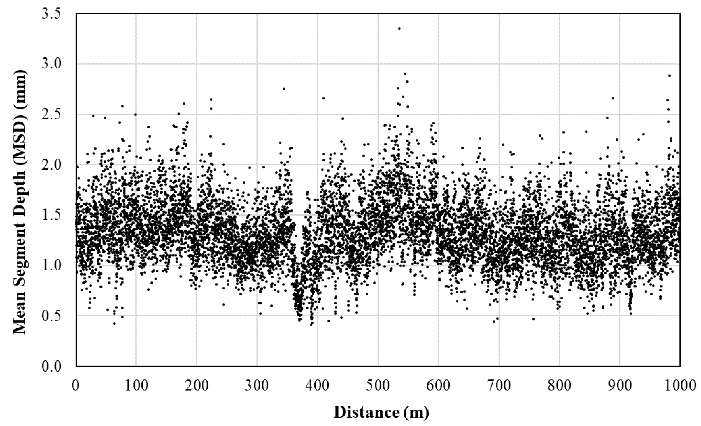
Notice that an actual chip seal project can be up to several tens of kilometers long. An acceptance test typically produces around 20,000 MSD values in each direction, totaling 40,000 MSD values for a 1.0-kilometer-long chip seal. Figure 1 displays the MSD values measured along an actual 1.0-kilometer-long chip seal with an MPD of 1.131 mm and a standard deviation of 0.337 mm. Evidently, a single MPD may fail to capture the full range of texture variations within the surface and detect localized variations that affect the chip seal’s performance. By leveraging machine learning techniques, however, it becomes feasible to address inconsistencies or outliers present in the data, extract pertinent features from the data that hold significant implications for chip seal performance, and establish a well-defined threshold for the purpose of anomaly detection.

4. Methodology

4.1. Data Preparation and Processing

To establish a rigorous quality control procedure for chip seal construction, four distinct datasets were developed: the MSD dataset, the MPD dataset, the 1-mile wheel track outlier percentage dataset, and the unqualified One-mile wheel track percentage dataset. The MPD dataset, the One-mile wheel track outlier percentage dataset, and the unqualified One-mile wheel track percentage dataset are all derived from the foundational MSD dataset. The MSD and the MPD datasets were generated prior to data analysis, whereas the other two datasets were formulated during the analysis because they relied on results from previous analyses. Each dataset contains several columns to record various details, but only one numeric column in each is utilized as input for the models. All datasets were constructed using Python 3.9.

4.1.1. MSD dataset

The MSD dataset is constructed based on macro-texture profiles measured at 100 mm intervals. These profiles are acquired using two high-speed 100 kHz point lasers, which operate simultaneously to capture macro-texture profiles in both the right and left wheel tracks, as mentioned earlier. For each chip seal project, macro-texture profiles were collected from both wheel tracks of each lane. Thus, a bidirectional roadway yielded four distinct profiles, whereas a dual carriageway generated eight. As such, the MSD dataset captured macro-texture profile data from every wheel track across all lanes and directions. This data is consolidated into a single column in the dataset, with each value corresponding to specific wheel track and direction information. In addition to the macro-texture data, the MSD dataset also includes additional relevant project details, such as road names, years of construction, and districts. Each district has millions of data entries captured within the MSD dataset.

4.1.2. MPD dataset

While the MSD dataset provides an exhaustive view of the macro-texture of the chip seal surface, its size is vast, with millions of MSD data entries for each district, as shown in Table 3. Although machine learning is inherently data-intensive, the sheer volume of this dataset can challenge even high-capacity computer hardware. Therefore, this study undertook further data refinement based on the MSD datasets. In Indiana, friction numbers are measured using the LWTS typically at the standard test speed of 40 mph, approximately equivalent to 20 m/s. Consequently, this research chose a 20 m interval for MPD calculation. Within a 20 m segment, 200 sequential MSD values are observed. For every wheel track, in each lane and direction, the average of these 200 consecutive MSD values within a 20 m segment is calculated to derive a single MPD value, which will be referred to as MPD₂₀ hereafter. The MPD dataset subsequently compiles these MPD₂₀ values, along with relevant details such as wheel track, direction, road name, chip seal project completion year, and district information. After this preprocessing, the sizable MSD dataset is reduced to tens of thousands of entries for each district, as delineated in Table 3. The MPD dataset was then used as input for the anomaly detection model. For consistency, all data points in the MPD dataset underwent a standardization procedure, ensuring the values were normalized to a consistent scale.

4.1.3. One-mile wheel track outlier percentage dataset

Utilizing the MPD dataset, the anomaly detection model enabled the generation of a distinct range of normal values for each district. This range facilitates a preliminary assessment of chip seal projects’ quality by discerning between typical values and outliers within the vast MSD dataset. However, a straightforward calculation of the outlier percentage for an entire district or an individual chip seal project is overly generalized. Hence, this research emphasizes the significance of more granular evaluations and chooses to calculate outlier percentages over one-mile stretches using the MSD dataset. Over a segment of 1 mile, an estimated 16,093 MSD values are recorded. With the predefined range of normal values in hand, these data can be systematically categorized into either ‘normal’ or ‘anomaly’ groups. This categorization then aids in the precise computation of the outlier percentage. Marrying these outlier percentages with supplemental details—such as wheel track, direction, road number, chip seal project completion year, and district data—culminates in the formation of the ‘one-mile wheel track outlier percentage dataset’. This particular dataset serves as a cornerstone for the initial phase of chip seal projects’ quality acceptance.

4.1.4. Unqualified one-mile wheel track percentage dataset

While assessing the quality of a single one-mile wheel track provides valuable insight, it does not necessarily reflect the overall quality of the entire chip seal project. As a result, the unqualified one-mile wheel track percentage dataset was established. This dataset is derived by computing the unqualified rate for each one-mile wheel track across every lane and direction within a specific chip seal project. Given that a chip seal project usually covers several one-miles on each wheel track, it is crucial that a sufficient number of these segments meet the predefined quality acceptance standard outlined in this study. In addition to the percentages of unqualified one-mile wheel track, this dataset also includes details such as wheel tracks, directions, road names, years of chip seal construction, and districts.

4.2. DBSCAN-Isolation Forest Model

4.2.1. Density-based spatial clustering of applications with noise

The Density-Based Spatial Clustering of Applications with Noise (DBSCAN) algorithm is recognized as a prominent density-driven clustering technique, acclaimed for its ability to detect clusters of diverse geometric configurations within a dataset [25,26]. It is typically utilized in the transportation sector to interpret traffic patterns, identify congested regions, and predict potential traffic incident zones. The application of DBSCAN has recently extended to the determination of pavement friction performance ratings alongside other clustering techniques [27]. Beyond its clustering capabilities, DBSCAN is also adept at anomaly detection. Its capability to differentiate regions of typical data behavior from points that deviate from these patterns makes it particularly efficient in detecting and isolating anomalous data points. Unlike other clustering methods, DBSCAN does not necessitate a predefined number of clusters, enhancing its proficiency in detecting noise across diverse datasets.

Two critical hyperparameters, epsilon (ε) and the minimum number of points (minPts), are essential for DBSCAN algorithm’s performance in noise detection. The epsilon (ε) parameter defines the neighborhood radius of a given data point, while the minPts specifies the minimum number of data points required within this radius (ε) for the designated point to be characterized as a core point. Data points that do not reside within the ε radius of a core point and do not satisfy the minPts criterion are typically classified as outliers. For evaluation the performance of the DBSCAN’s outcome, the silhouette score can be employed. The score is a metric to gauges the efficacy of the clustering algorithm and is given by the following formula:

s = \frac{b - a}{\max (a, b)}

(5)

where s = silhouette score; a = the mean distance between an item and all other items in its cluster; b = the mean distance between an item and all other items in the next nearest cluster. The silhouette score ranges between -1 and 1. A score closer to -1 indicates inadequate clustering separation, implying that the clusters are not distinct. On the other hand, a score nearer to 1 suggests that the data points are well-clustered and have a strong cohesion within clusters. A score hovering around 0 indicates ambiguous clustering, meaning that data points might be close to the boundaries of their clusters [25,26].

4.2.2. Isolation Forest algorithm

The Isolation Forest is primarily employed for anomaly detection and operates as an unsupervised machine learning algorithm [28]. It functions on the principle of 'isolation', aiming to isolate specific instances rather than group conventional data points. At its core, the algorithm involves creating individual isolation trees, which together form an ensemble known as the Isolation Forest. The construction of the tree hinges on decisions influenced by the dataset’s structure. In every iteration of the iterative process, a feature is chosen at random. A split criterion is then determined by selecting a random value between that attribute’s minimum and maximum values. This inherent randomness ensures variability within the trees, thereby aiding in distinguishing anomalies from normal data points. As the process of random feature selection and splitting continues, new tree nodes emerge with each division. The recursion terminates in two cases:

when a node contains only a single data instance, rendering further splits redundant
when the tree reaches a predetermined maximum height, a measure to prevent overfitting.

Once constructed, these individual trees are combined to form an Isolation Forest, enhancing the accuracy of anomaly detection and ensuring a more comprehensive scope of application.

In determining the potential anomaly of a specific data instance, it is paramount to compute the path length that’s essential for isolating the sample. The path length is defined as the number of edges a sample traverses within the hierarchical tree, starting from the root node and ending at its terminal counterpart. Typically, anomalies are associated with shorter path lengths in the tree, whereas normal data points tend to have longer paths. To evaluate the distinctiveness of an instance compared to others, based on their respective path lengths, the computation of an anomaly score becomes indispensable. Mathematically, the anomaly score can be formulated as follows:

s (x, n) = 2^{- \frac{E (h (x))}{c (n)}}

(6)

where s(x,n) = anomaly score; n = the size of the dataset; E(h(x)) = the average path length of instance x over a collection of trees; c(n) = the average path length of unsuccessful search in a binary search tree given n samples, defined as:

c (n) = 2 H (n - 1) - \frac{2 (n - 1)}{n}

(7)

where H(i) = the harmonic number and can be approximated by ln(i) + 0.5772156649 (Euler's constant). The anomaly score ranges between [0,1]. A score close to 1 indicates an anomaly; scores below 0.5 points to normality; and scores nearing 0.5 imply that the dataset might not have clear anomalies [28].

4.2.2. DBSCAN-Isolation Forest model

Both the DBSCAN and Isolation Forest algorithms offer powerful tools for outlier detection, yet each comes with its unique set of challenges. For example, the results of DBSCAN might not always align with domain-specific criteria, as points accessible from multiple clusters could belong to any one of those clusters. On the other hand, the Isolation Forest tends to be sensitive to certain hyperparameters, such as the number of trees. Recognizing the strengths and limitations of both, integrating DBSCAN and Isolation Forest yields a harmonized model that fuses density-based clustering with random forest-based anomaly detection. Termed ‘DBSCAN-Isolation Forest’ in this context, this hybrid approach is especially adept at handling datasets marked by density variations and a spectrum of anomalies. Given the unique traits of the MPD dataset, particularly its density fluctuations and anomaly features, this study employed the DBSCAN-Isolation Forest hybrid for identifying irregularities in macro-texture profiles.

In implementing the DBSCAN-Isolation Forest model on the MPD dataset, the process started with an initial clustering stage using DBSCAN. This step leverages the density-centric capability of DBSCAN to outline regions of high data concentration, identifying both points of interest and potential zones containing noise or outliers. Points flagged by DBSCAN as potential outliers are subsequently fine-tuned using the Isolation Forest. The secondary step uses the Isolation Forest algorithm to verify the outlier status of these points, providing a confirmation of their anomalous nature. Moreover, the extent of their deviation can be quantified based on the resultant anomaly score. The synergy between DBSCAN and Isolation Forest becomes evident, especially when dealing with data exhibiting significant density variations. This is a scenario where relying solely on DBSCAN could prove inadequate. The hybrid model enhances the identification process by examining points initially marked as potential outliers by DBSCAN and further refining their status with the Isolation Forest.

The DBSCAN-Isolation Forest model was instantiated using Python 3.9 and employed the scikit-learn (sklearn) library [26]. The refinement of the DBSCAN model is achieved by assessing the silhouette coefficient. The hyperparameter associated with a silhouette coefficient approaching 1 is chosen. When implementing the Isolation Forest model using the scikit-learn library, two essential hyperparameters must be specified: "contamination" and the number of trees. The term "contamination" specifies the proportion of outliers in the dataset. It sets a threshold for designating observations as outliers. For example, when contamination is set to 0.1, the algorithm assumes that 10% of the data consists of outliers. While this hyperparameter did not exist in the original model, its introduction aimed to enhance user-friendliness and practicality. Given that the Isolation Forest is based on an ensemble of randomized decision trees, the number of trees is another pivotal hyperparameter. In this study, the optimum Isolation Forest hyperparameters were identified by computing the cumulative anomaly score. The dataset was split into two subsets, a training set and a validation set, for hyperparameter fine-tuning. The parameter configuration that produced the lowest overall anomaly score for the validation set was regarded as optimal and was selected for anomaly detection.

4.3. Statistical Methods for Quality Control

4.3.1. Analysis of variance

Macro-texture profiles were obtained using two high-speed 100 kHz point lasers operating in tandem, systematically recording the macro-texture in both the right and left wheel tracks. As a result, all datasets sourced from these initial profiles incorporate information gathered simultaneously from both tracks. A one-way analysis of variance (ANOVA) was employed to ascertain if there were significant disparities in outlier percentages between 1-mile road segments of the right wheel track and its counterpart on the left. If no prominent differences emerge, the outlier percentages from both tracks will be amalgamated, forming the input for ensuing analyses.

In a one-way ANOVA, the null hypothesis (H0) posits that there is no significant difference between the means of the groups under comparison. Conversely, the alternative hypothesis (H1) asserts that a significant difference exists between the means of at least two of the groups. The F-test, used in the ANOVA, contrasts the ratio of variation between groups to the variation within groups [29]. Equations 8-12 illustrate the procedures to calculate F-statistics for ANOVA.

S S R = \sum n_{i} {(\bar{Y_{i}} - \bar{Y})}^{2}

(8)

S S E = \sum \sum {(Y - \bar{Y_{i}})}^{2}

(9)

d f_{1} = k - 1

(10)

d f_{2} = N - k

(11)

F = \frac{S S R / d f_{1}}{S S E / d f_{2}}

(12)

where

n_{i}

= the sample size in the ith group; (

\bar{Y_{i}}

) = the sample mean in the i^th group;

\bar{Y}

= the overall mean; Y = an observed data; k = the number of independent groups; N = the total number of observations in the analysis; SSR = regression sum of squares; SSE = sum of squares of errors. The F-statistics can be used to calculate the associated p-value, which is then compared to the predetermined significance level, typically set at 0.05. If the p-value obtained from the test is less than this significance level (e.g., p < 0.05), the null hypothesis is rejected in favor of the alternative hypothesis, suggesting a statistically significant difference between the group means. Conversely, if the p-value exceeds this critical threshold, the null hypothesis is retained, signifying no significant differences between the groups under examination [29].

4.3.2. Proportion control chart

The proportion control chart (P-chart) is a statistical tool utilized for monitoring the proportion of nonconforming items (e.g., defects or failures) within a predefined sample [30]. In this study, the P-chart framework is harnessed to establish threshold criteria that demarcate the quantification status of a chip seal project.

In the implementation of the P-chart method, the initial step involves ascertaining the proportion of defects. In this study, this is represented as the percentage of anomalies over a 1-mile long wheel track or unqualified 1-mile wheel track rate in a chip seal project. The proportion can be determined through the following formula:

p = \frac{N u m b e r o f o u t l i e r}{T o t a l s a m p l e n u m b e r}

(13)

In this formula, p = the proportion of anomalies. Throughout the analytical process, the calculated p values are employed to derive the center line (CL), upper control limit (UCL), and lower control limit (LCL) for the chart, as shown in Equations 14-16.

C L = \bar{p}

(14)

U C L = \bar{p} + 3 \sqrt{\frac{\bar{p} (1 - \bar{p})}{n}}

(15)

L C L = \bar{p} - 3 \sqrt{\frac{\bar{p} (1 - \bar{p})}{n}}

(16)

where n = the sample size, which is the aggregate count of outlier percentages in the dataset;

\bar{p}

= the average value of p [30].

5. Results and Analysis

5.1. Anomaly Detection

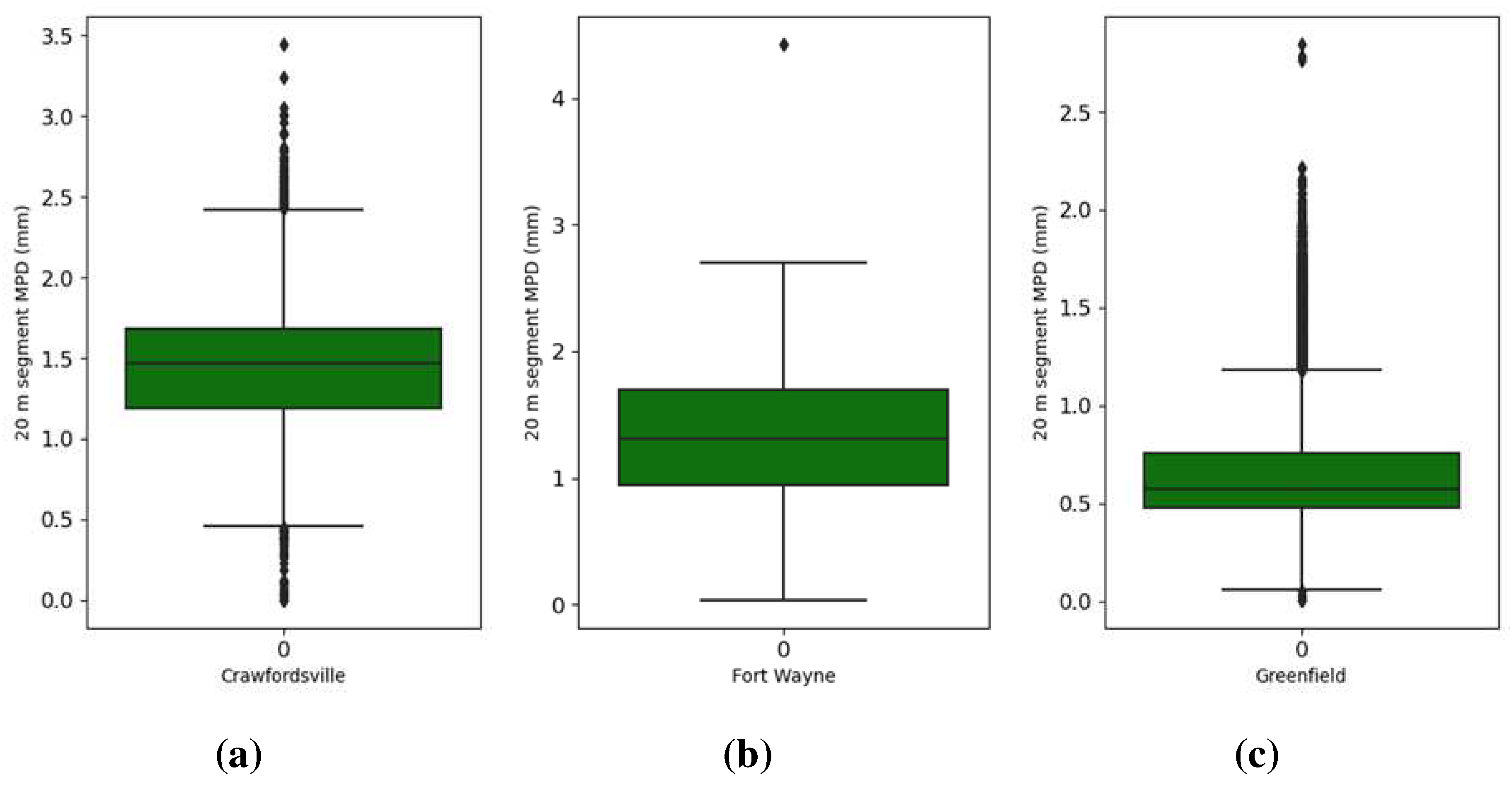
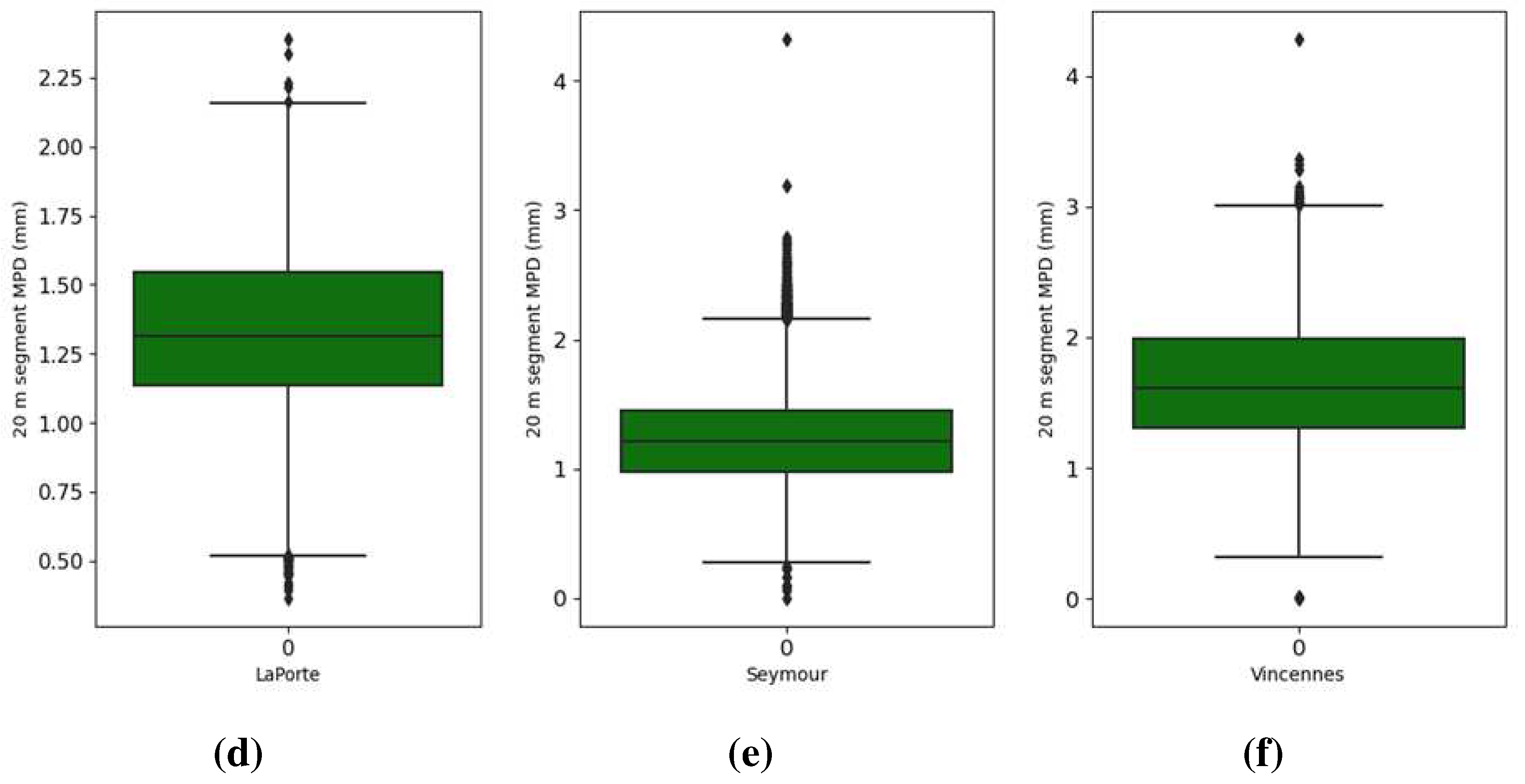
Due to the regional variations in the utilization of aggregates and asphalt emulsions, the detected anomalies across these regions exhibit significant disparities. Figure 2 presents the Box-whisker plots delineating the MPD₂₀ values across various districts. The Box-whisker plot is a conventional method of visually representing data distribution based on a five-number summary: the minimum, first quartile, median, third quartile, and the maximum values. As shown in Figure 2, barring Greenfield and Vincennes, the quartiles at 25th, 50th, and 75th percentiles for the MPD₂₀ across the other four districts predominantly lie within the values of 1 mm, 1.3 mm, and 1.5 mm, respectively. In stark contrast, Greenfield exhibits a reduced range with its 75th percentile of MPD₂₀ being less than 0.76 mm, while Vincennes presents relatively elevated MPD₂₀ values, where 97.5% exceed 0.77 mm. The observed variability in the MPD₂₀ distribution across districts underscores the imperative to conduct distinct anomaly detections tailored to each region.

In the construction of the DBSCAN-Isolation Forest model tailored for the six specific districts?Crawfordsville, Fort Wayne, Greenfield, Laporte, Seymour, Vincennes?the hyperparameters ε and minPts within the DBSCAN component were fine-tuned. The resultant parameters for each district are as follows: Crawfordsville (0.1, 5), Fort Wayne (0.1, 2), Greenfield (0.3, 2), Laporte (0.3, 2), Seymour (0.1, 10), and Vincennes (0.3, 2). For the Isolation Forests across all districts, the parameters for ‘contamination’ and ‘number of trees’ were set to: Crawfordsville (0.1, 150), Fort Wayne (0.15, 150), Greenfield (0.1, 100), Laporte (0.15, 150), Seymour (0.1, 100), and Vincennes (0.15, 150), respectively. 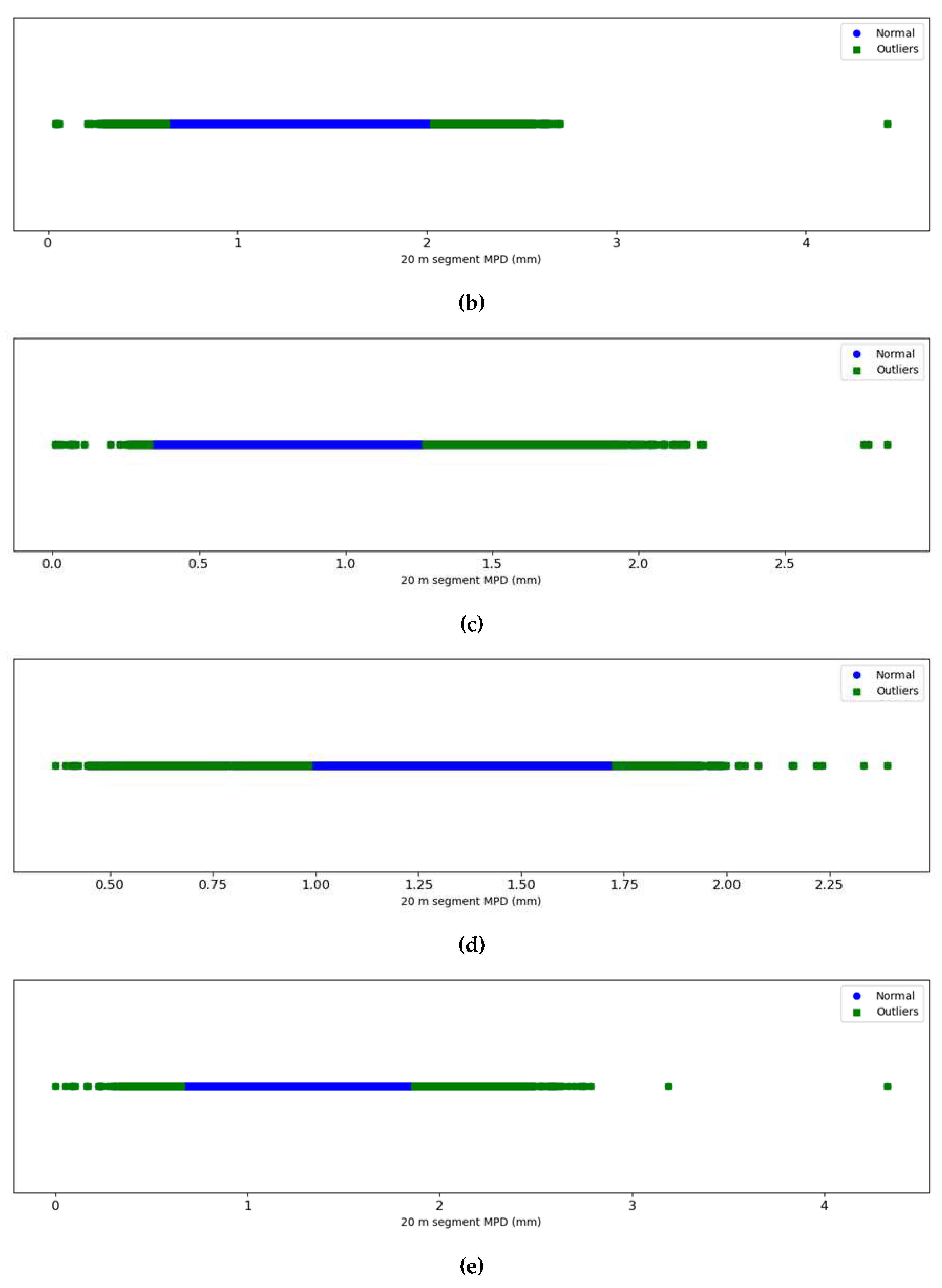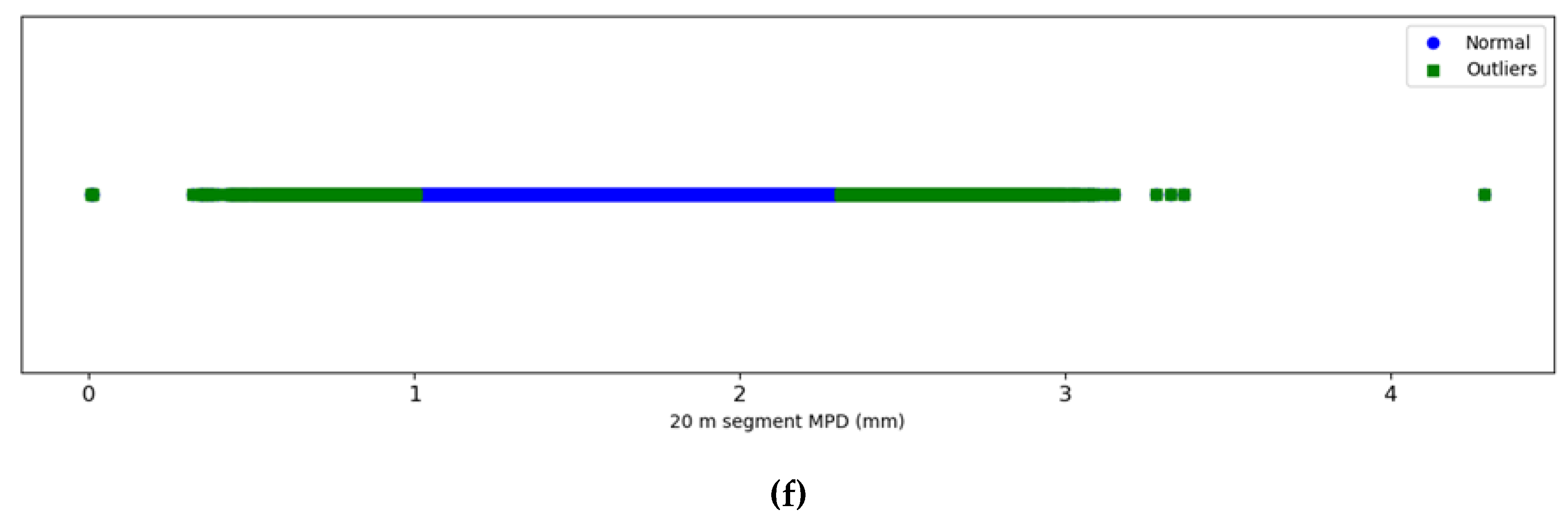Figure 3 portrays the distribution of both normal data and outliers of each district. On the horizontal axis, MPD₂₀ values are represented. Outliers are marked in green, while normal data points are in blue. This visualization underscores the capability of the utilized algorithm to discern extremely high or low MPD₂₀ values as outliers, contingent on each district's unique data characteristics. Practically, excessively high or low MPD₂₀ values can either influence ride quality or result in decreased friction. The typical MPD₂₀ values for each district, rounded to one decimal place, are showcased in Table 4. An MPD₂₀ or MSD value that deviates from its district's typical range suggests that it's an outlier.

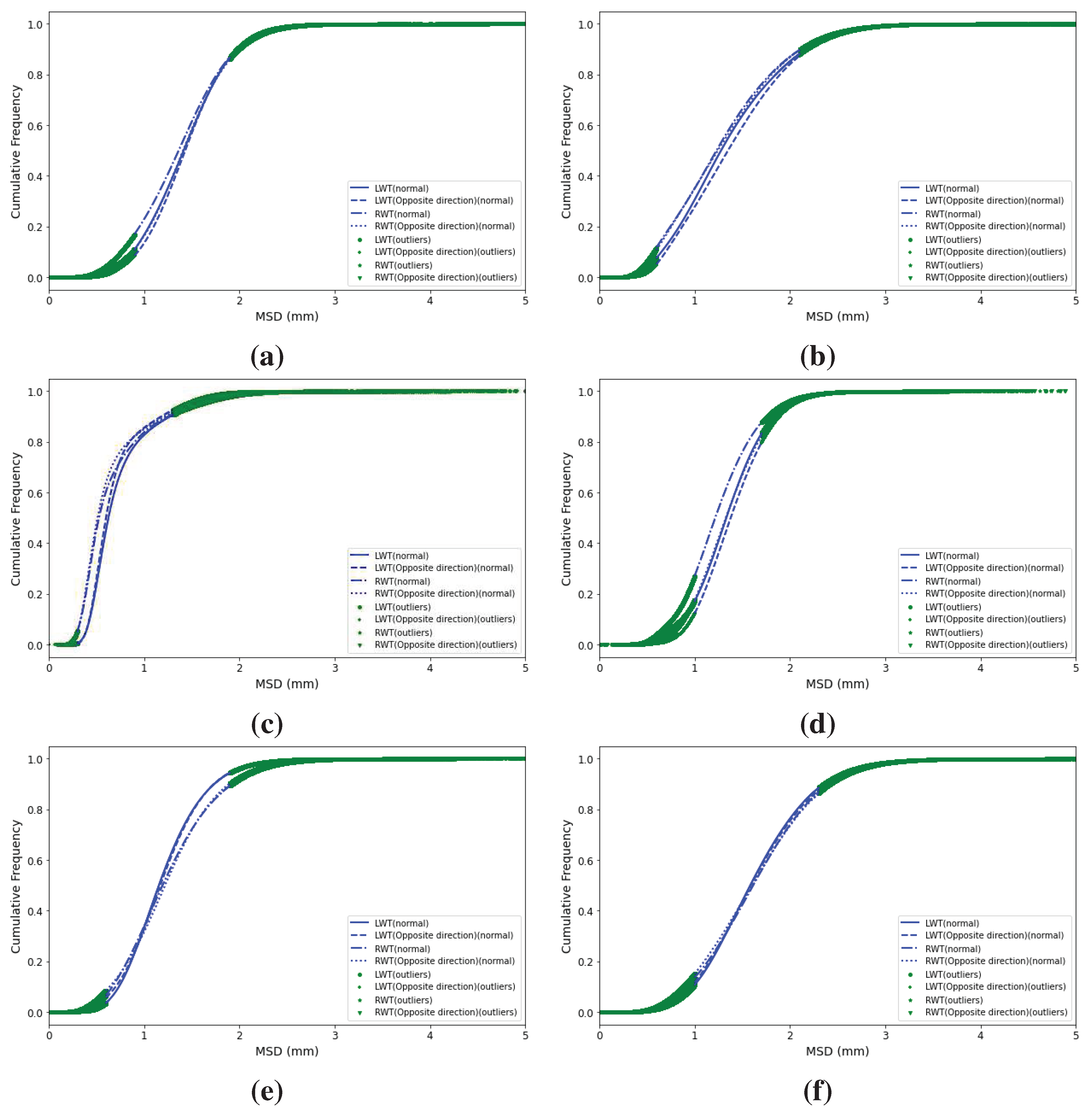
In Figure 4, the cumulative frequency distribution (CFD) is depicted, showcasing both the normal and outlier values of each district. This distribution is further stratified by wheel tracks and directions. The CFD provides a cumulative frequency for each category within a dataset. This approach offers a simplified visualization for large texture datasets, making it easier to identify subtle variations in the texture measurement distribution. In this study, CFDs were utilized to analyze variations between MSD values in the right and left wheel paths in both directions. On the CFD graph, the horizontal axis denotes MSD (mm), while the vertical axis showcases the cumulative frequency. A shift to the right on this graph indicates an increase in texture depth. Post anomaly detection, the CFDs of each region revealed data retention between 60% and 90%. Excluding the Crawfordsville and LaPorte districts, the CFDs from other regions demonstrated consistent patterns between the left wheel tracks in both directions and the right wheel tracks in both directions. However, a slight divergence was observed between the CFDs of the left and right wheel tracks. In the case of the Crawfordsville and LaPorte districts, a distinct disparity was noted in the CFD of the opposing right wheel tracks. Notably, the CFDs of different wheel tracks largely overlapped in the same district across varying directions, suggesting analogous patterns in data distribution. As a result, subsequent analyses in this study will separately address the quality control of the chip seal project from the perspective of the left and right wheel tracks.

5.2. Quality Control

The quality control process consists of two steps. First, establish the outlier percentage threshold for each 1-mile road segment per wheel track. Second, determine the maximum acceptable proportion of unqualified 1-mile wheel track segments within the overall scope of the chip seal project’s quality acceptance.

For the first stage of quality control, a dataset detailing the outlier percentage of each one-mile segment was constructed from anomaly detection results. The dataset comprises 2,059 data entries, with 1037 representing outlier percentages for left wheel tracks and 1,022 for right wheel tracks. According to the previous analysis, a one-way ANOVA test was employed to determine whether there exists a significant difference between the left and right wheel track data. If the analysis yields no statistically significant differentiation between the two datasets, they will be consolidated for subsequent evaluation; otherwise, they shall remain segregated. At a significance level of 0.05 for the ANOVA test, the resulting p-value is 3.27 × 10-9, considerably below the stipulated threshold. This underscores a pronounced difference between the outlier percentages of the right and left wheel tracks. As such, combining the two groups of data is inadvisable. Each of the two data groups was analyzed separately in the preliminary quality control procedure. 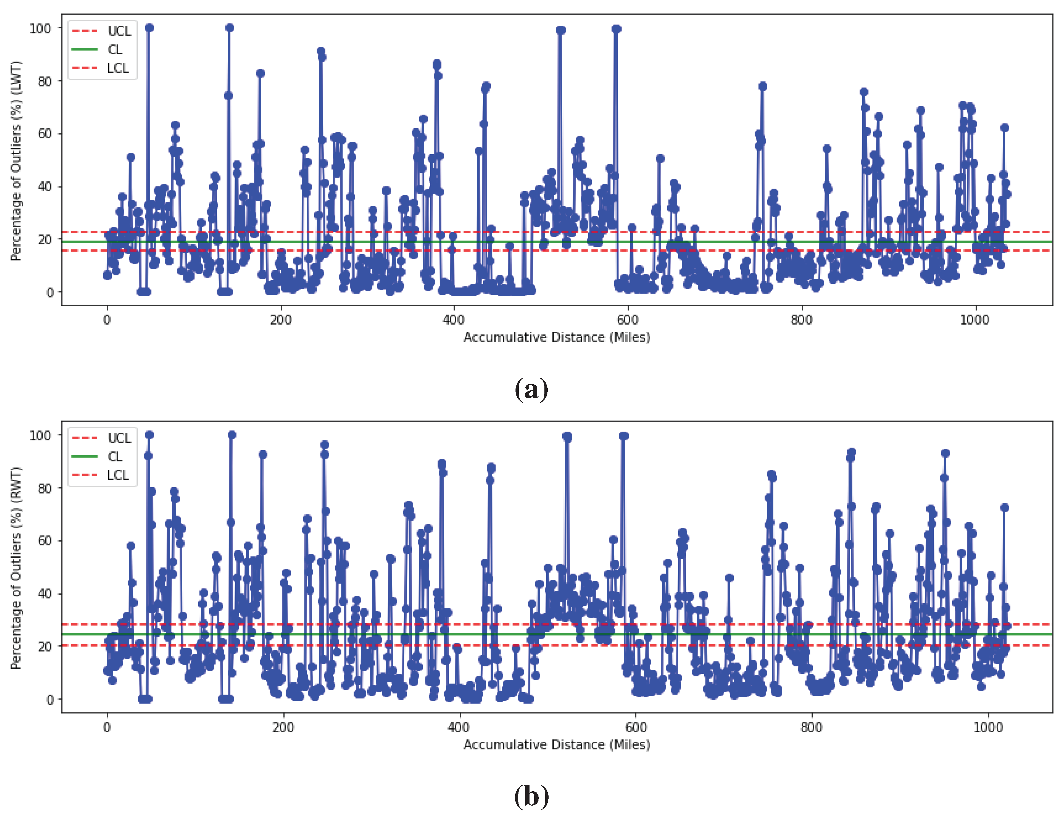Figure 5 depicts the P-charts for both the left and right wheel tracks. The horizontal axis denotes the cumulative distance, derived from the aggregated distances of individual projects. The vertical axis signifies the percentage of outliers. In both Figure 5a,b, three distinct lines are present. The red dashed lines represent the upper and lower control limits. These demarcations aid in assessing the process variability. Data points lying beyond these boundaries indicate potential deviations from the expected process control. The solid green line delineates the center line, signifying the mean value of the entire dataset under examination. Despite the ANOVA results indicating significant differences between the outlier percentages of the left and right wheel tracks, both Figure 5a,b reveal that upper control limit approximates 25%, while the lower control limit is around 18%. The results can be interpreted as follows: For both the 1-mile segment of the left and right wheel tracks, an outlier percentage below 18% represents exceptional chip seal performance on the designated road section. A value between 18% and 25% signifies that the chip seal quality on the segment is within acceptable limits. However, an outlier percentage that exceeds 25% points to a subpar chip seal quality for that specific road segment. Therefore, the threshold for the outlier percentage of 1-mile wheel track is firmly established at 25%.

The subsequent stage in the quality control process is determining the acceptable upper limit for the unqualified 1-mile wheel track rate within a chip seal project. The dataset for this was formed by calculating unqualified rate for 1-mile wheel tracks across all lanes and directions within a chip seal project. A "qualified" wheel track is one with a 1-mile outlier percentage below 25%. In total, 350 sets of data were collected. This dataset encompassed percentages of unqualified 1-mile wheel tracks, derived from 1-mile outlier percentages for wheel tracks in both directions. Additional data points included road names, the year of chip seal project completion, and districts. Figure 6 presents the P-chart displaying the proportion of unqualified 1-mile wheel tracks for individual chip seal projects. The lower control limit is set as approximately 30%, indicating that projects under this line have fewer than 30% of their 1-mile wheel tracks deemed unqualified. Conversely, the upper control limit, established at 50%, signifies that projects exceeding this benchmark have more than 50% of their 1-mile wheel tracks deemed unqualified. In evaluating the quality acceptance of a project, the performance of each wheel track must be considered. From the result, it can be deduced that a project in which fewer than 30% of its 1-mile wheel tracks are deemed unqualified is of good quality. Projects with an unqualified rate between 30% and 50% for their wheel tracks are deemed acceptable, with the upper threshold of acceptability set at 50%. Any project with a 1-mile wheel track unqualified rate exceeding this limit is categorized as unsatisfactory, necessitating additional assessment and scrutiny.

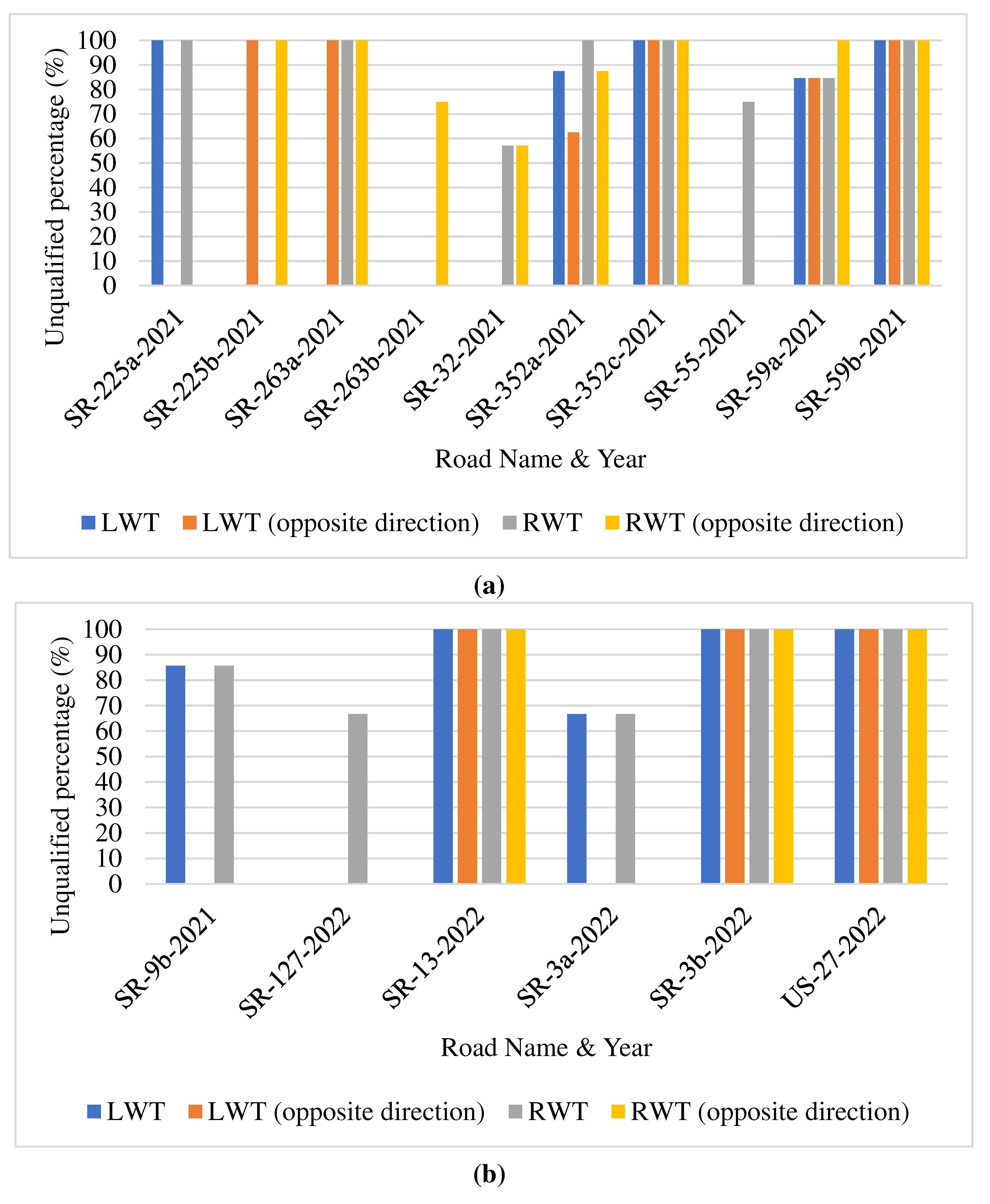
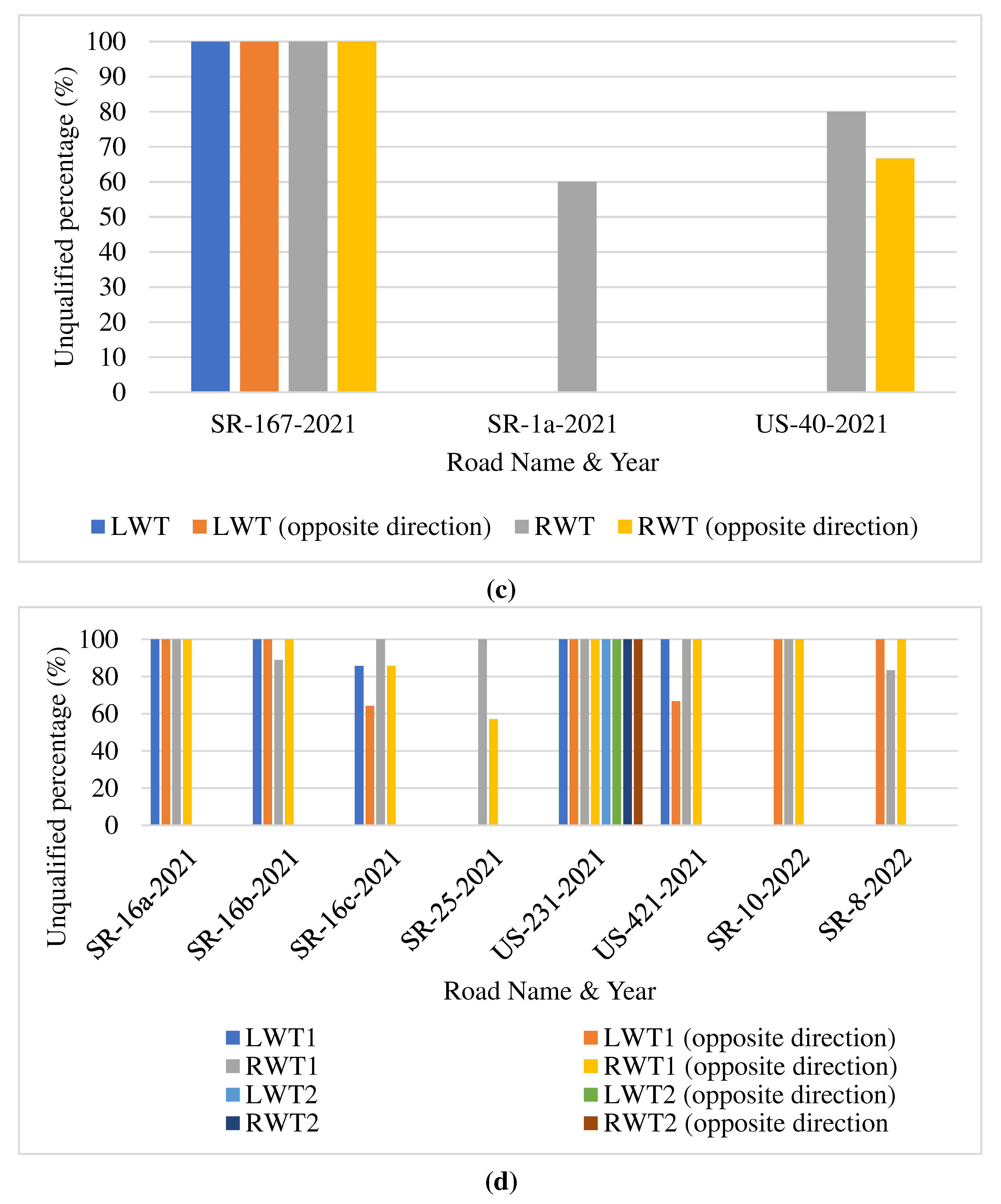
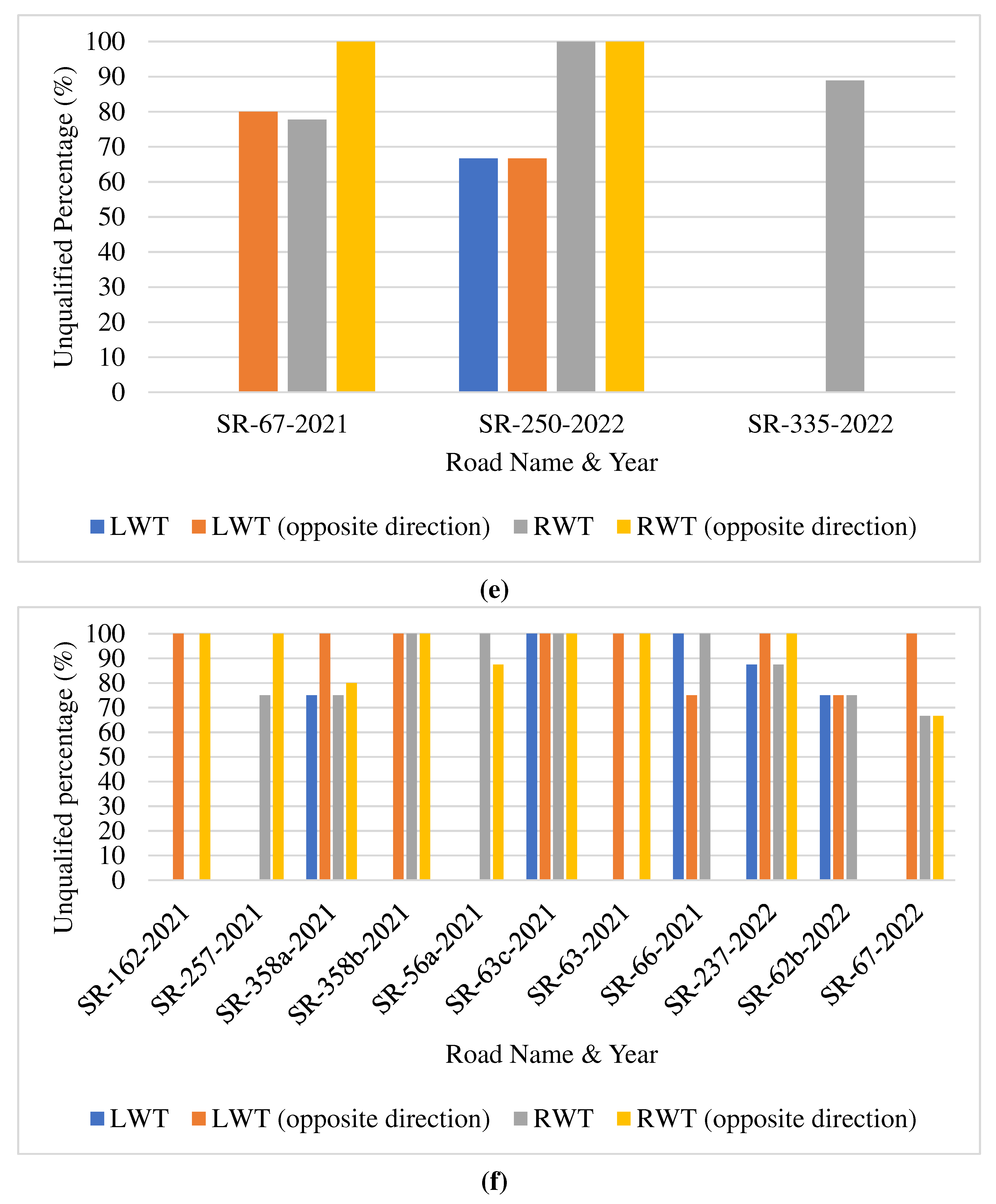
Figure 7 depicts projects of each district with an unqualified 1-mile wheel track rate greater than 50%. Referring to Figure 7a, between 2021 and 2022, ten chip seal projects in Crawfordsville failed to meet the quality acceptance criteria proposed by this study. Of these, SR-263, SR-352, and SR-59 are of particular concern, having a 100% unqualified 1-mile wheel track rate for both right and left wheel tracks in both directions. In Fort Wayne, as illustrated in Figure 7b, six projects fell short of the standards. SR-13, SR-3, and US-27 are especially concerning due to their performance metrics. In Greenfield (Figure 7c), three projects did not conform. Notably, SR-167 exhibited a 100% unqualified rate for both tracks in both directions. LaPorte had seven projects that fell below the criteria, with SR-16, SR-231, SR-421, SR-10, and SR-8 deserving special attention, as presented in Figure 7d. In Seymour (Figure 7e), roads SR-67 and SR-250 warrant immediate inspection out of the three projects. In Vincennes, SR-358, SR-63, and SR-237 call for further scrutiny out of the 11 projects, as shown in Figure 7f. While these conclusions are based on specific data attributes, the proposed quality control criteria offer engineers a foundational benchmark for evaluating chip seal projects.

5.3. Validations

To validate the efficacy of the proposed anomaly detection and quality control methodologies, four chip seal sections (see Table 5) from three different districts were selected for field inspection and friction testing. These chip seals were identified as problematic in the preceding section. Examination of each wheel track’s characteristics in the projects revealed the following:

In Section 1, a predominant portion of MSD outliers exceed Fort Wayne’s 2.1 mm threshold. Notably, 97.5% of outliers in the northbound lane surpass this limit across all wheel tracks. In the southbound lane, approximately 97.5% of outliers in the left wheel track and 95% in the right wheel track exceed the 2.1 mm threshold. The above suggests that the surface texture may be very rough.
In Section 2, over 95% of MSD outliers fall below the 0.6 mm threshold, encompassing all directions and tracks, which indicates a possible slippery surface.
In Section 3, the 97.5th percentile of outliers for each wheel track falls below Seymour’s 0.6 mm mark, implying a potential slippery surface.
In Section 4, the 2.5th percentile of MSD outliers for each wheel track exceeds 2.3 mm, indicating a surface with a rough texture.

Despite unique outlier distributions across different chip seal projects, wheel tracks in the same direction within a single project exhibit uniform characteristics. Subsequent analyses combined outliers from all the four wheel tracks, focusing on the associated road section's friction. This process aims to further validate the proposed quality control methodology's efficacy. Table 5 displays the percentages of outliers (larger than the maximum threshold values and lower than the minimum threshold values of a specific district) and friction measurements of the 4 sections. Based on the table, Section 1, Section 3, and Section 4 exhibit substantial outlier proportions, predominantly over 40%. Among them, Section 1 and Section 4 notably surpass the upper 20 m MPD threshold of the corresponding districts. On the other hand, Section 2 and Section 3 exhibited a pronounced percentage of outliers below the minimum 20 m MPD threshold of their districts. The friction numbers measured using the LWST are also presented in Table 5. The chip seals in Section 1 and Section 4 demonstrated remarkably high friction. 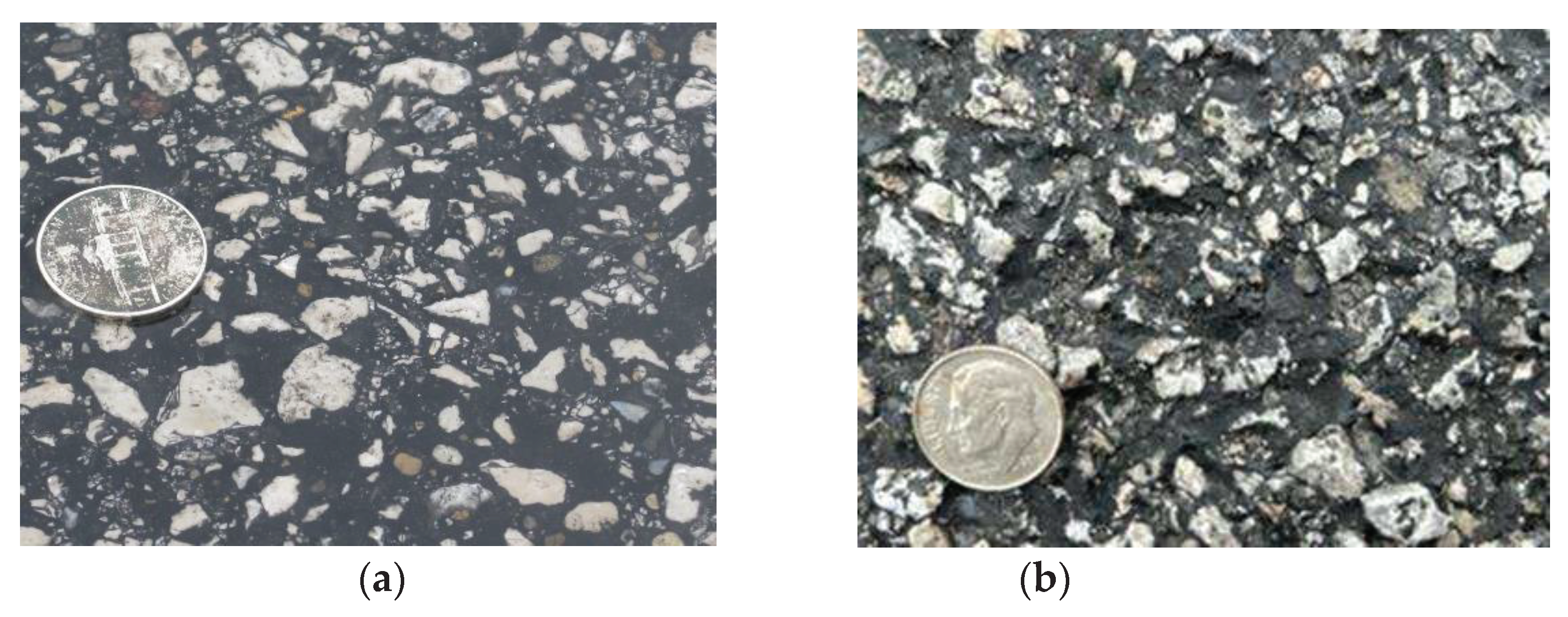In contrast, the chip seals in Section 2 and Section 3 experienced very low friction. Further field visual inspection revealed chip seal surfaces with both very low and very high friction, as depicted in Figure 8. Evidently, both field inspections and friction measurements align closely with the results generated by the proposed methodologies.

6. Conclusion

To address the challenges associated using MPD measurements for the quality control of chip seal construction, this study employs a hybrid machine learning model, the DBSCAN-Isolation Forest model, to conduct anomaly detection on a dataset of 183,794 values spanning six districts in Indiana. This innovative model adeptly pinpoints MPD values that significantly diverge from the expected range, delivering invaluable insights in an unsupervised context. The typical MPD ranges of the six districts are as follows: Crawfordsville [0.9, 1.9], Fort Wayne [0.6, 2.1], Greenfield [0.3, 1.3], LaPorte [1.0, 1.7], Seymour [0.6, 1.9], and Vincennes [1.0, 2.3].

Subsequently, this research introduces a two-step quality control procedure tailored for chip seal evaluation. In its preliminary stage, the analysis involves computing the outlier percentage across each 1-mile segment for all wheel tracks. Leveraging proportion control chart methodologies, this investigation concludes that within a 1-mile stretch, the outlier percentage for any wheel track should not surpass the 25% mark. In the subsequent stage, the research gauges the unqualified rate of 1-mile wheel track segments throughout various projects. By harnessing the proportion control chart technique once more, a decisive threshold of 50% was derived. This signifies that for any wheel track segment, the 1-mile unqualified rate should not breach the 50% threshold. Surpassing this delineated boundary calls for an intensified, detailed assessment. Both field inspections and friction measurements align closely with the results generated by the proposed methodologies.

While the findings of this study are intrinsically anchored to particular data characteristics, it is contended that the presented quality control framework equips pavement construction practitioners with a preliminary evaluative standard for chip seal undertakings.

Author Contributions

Conceptualization, Shuo Li and Jieyi Bao; methodology, Jieyi Bao, Joseph Adcock, and Shuo Li; software, Jieyi Bao and Joseph Adcock; validation, Jieyi Bao, Joseph Adcock, and Shuo Li; formal analysis, Jieyi Bao, Joseph Adcock, and Shuo Li; investigation, Jieyi Bao, Joseph Adcock, and Shuo Li; resources, Yi Jiang and Shuo Li; data curation, Joseph Adcock, Jieyi Bao, and Shuo Li; writing—original draft preparation, Jieyi Bao and Shuo Li; writing—review and editing, Yi Jiang and Shuo Li; visualization, Jieyi Bao and Shuo Li; supervision, Yi Jiang and Shuo Li; funding acquisition, Shuo Li and Yi Jiang. All authors have read and agreed to the published version of the manuscript.

Funding

This research was supported in part by Joint Transportation Research Program between Purdue University and Indiana Department of Transportation, grant number SPR-4646.

Data Availability Statement

Data used in this paper is available upon request.

Conflicts of Interest

The authors declare no conflict of interest. The funders had no role in the design of the study; in the collection, analyses, or interpretation of data; in the writing of the manuscript; or in the decision to publish the results.

References

Shuler, S. , Lord, A., Epps-Martin, A., and Hoyt, D. Manual for Emulsion-Based Chip Seals for Pavement Preservation. NCHRP Report 680, Transportation Research Board, Washington, DC, USA, 2011. [CrossRef]
INDOT. Chip Sealing. Indiana Department of Transportation: Indianapolis, IN, USA. https://www.in.gov/indot/maintenance-operations/. Accessed 08/09/2023.
Gransberg, D. , and James, D. Chip Seal Best Practices. NCHRP Synthesis 342, Transportation Research Board, Washington, DC, USA, 2005. [CrossRef]
Chipsealing in New Zealand. Transit New Zealand, Wellington, New Zealand, 2005.
Pavement Preservation Checklist Series 2: Chip Seal. Publication No. FHWA-HIF-19-02, Federal Highway Administration, 2019.
Li, S. , Shields, T. ( 2295(1), 11–18. [CrossRef]
Zhao, G. , Li, S., Jiang, Y., & Lee, J. Quality assurance procedures for chip seal operations using macrotexture metrics (Joint Transportation Research Program Publication No. FHWA/IN/JTRP2018/12). Purdue University: West Lafayette, IN, USA, 2018. [CrossRef]
Henry, J.J. Evaluation of Pavement Friction Characteristics. NCHRP Synthesis 291, Transportation Research Board, Washington, DC, USA, 2000.
Tobias, P. , de León Izeppi, E., Flintsch, G., Katicha, S., and McCarthy, R. Pavement Friction for Road Safety: Primer on Friction Measurement and Management Methods. FHWA-SA-23-007. Federal Highway Administration, Office of Safety, Washington, DC 20590, USA, 2023.
ASTM. ASTM E274/E274M-15. Standard Test Method for Skid Resistance of Paved Surfaces Using a Full-Scale Tire. ASTM: West Conshohocken, PA, USA, 2020.
ASTM. ASTM E303. Standard Test Method for Measuring Surface Frictional Properties Using the British Pendulum Tester. ASTM: West Conshohocken, PA, USA, 2022.
ASTM. ASTM E1911. Standard Test Method for Measuring Surface Frictional Properties Using the Dynamic Friction Tester. ASTM: West Conshohocken, PA, USA, 2019.
Kummer, H.W. , and Meyer, W.E. Tentative Skid-resistance Requirements for Main Rural Highways. NCHRP Report 37, Highway Research Board, Washington, DC, USA, 1967.
Li, S. , Zhu, K. Q., Noureldin, S., and Kim, D. Pavement surface friction test using standard smooth tire: The Indiana experience. In Transportation Research Board 83rd Annual Meeting Compendium of Papers (CD-ROM). Transportation Research Board, Washington, DC, USA, 2004.
Li, S. , Noureldin, S., and Zhu K. Q. Characterization of Microtexture on Typical Pavement Surfaces: A Pilot Study. Presented at 90th Annual Meeting of the Transportation Research Board, Washington, DC, USA, 2011.
ASTM. ASTM E965-15. Standard Test Method for Measuring Pavement Macrotexture Depth Using a Volumetric Technique. ASTM: West Conshohocken, PA, USA, 2019.
ASTM. ASTM E2157-15. Standard Test Method for Measuring Pavement Macrotexture Properties Using the Circular Track Meter. ASTM: West Conshohocken, PA, USA, 2019.
Zhao, H.; Wei, F.; Wang, C.; Li, S.; Shan, J. Determination of Friction Performance of High Friction Surface Treatment Based on Alternative Macrotexture Metric. Materials 2021, 14, 6895. [Google Scholar] [CrossRef] [PubMed]
Notes for the Specification of Bituminous Reseals, TNZ P17. Transit New Zealand: Wellington, New Zealand, 2002.
Adams, J. , Castorena, C, and Kim, Y.R. Construction quality acceptance performance-related specifications for chip seals. Journal of Traffic and Transportation Engineering (English Edition), Vol. 6, Iss. 4, 2019, 337-348, 2019. [CrossRef]
INDOT. Standard Specifications. Indiana Department of Transportation: Indianapolis, USA, 2020.
S. Li, K. S. Li, K. Zhu, S. Noureldin. Evaluation of friction performance of coarse aggregates and hot-mix asphalt pavements. Journal of Testing and Evaluation, 2007, 35(6), 571-577. [CrossRef]
Li, S. , Noureldin, S., and Zhu, Z. Upgrading the INDOT Pavement Friction Testing Program. Publication FHWA/IN/JTRP-2003/23. Joint Transportation Research Program, Indiana Department of Transportation and Purdue University, West Lafayette, Indiana, USA, 2004. [CrossRef]
ASTM. ASTM E1845-01. Standard Practice for Calculating Pavement Macrotexture Mean Profile Depth. ASTM: West Conshohocken, PA, USA, 2017.
Ester, M. , Kriegel, H.P., Sander, J., and Xu, X. A density-based algorithm for discovering clusters in large spatial databases with noise. Proceedings of 2nd International Conference on Knowledge Discovery and Data Mining. 1996, vol. 96(34), pp. 226-231.
Pedregosa, F. , Varoquaux, G., Gramfort, A., Michel, V., Thirion, B., Grisel, O., Blondel, M., Prettenhofer, P., Weiss, R., Dubourg, V., Vanderplas, J., Passos, A., Cournapeau, D., Brucher, M., Perrot, M., & Duchesnay, E. Scikit-learn: machine learning on Python. Journal of Machine Learning Research, 2011, vol. 12, pp. 2825-2830.
Bao, J. , Jiang, J., Li, S. Determination of Safety-Oriented Pavement-Friction Performance Ratings at Network Level Using a Hybird Clustering Algorithm. Lubricants, 2023, vol. 11(7). [CrossRef]
Liu, F.T. , Ting, K.M., and Zhou, Z.H. Isolation Forest. In 2008 Eighth IEEE International Conference on Data Mining. [CrossRef]
Kutner, M. H., C. J. Nachtsheim, J. Neter, W. Li. Applied Linear Statistical Models, Fifth Edition. McGraw Hill Education Private Limited, New York, 2013.
Montgomery, D.C. Introduction to Statistical Quality Control, Sixth Edition. John Wiley & Sons, Hoboken, New Jersey, 2009.

Figure 1. Mean segment depth (MSD) measurements on an actual chip seal.

Figure 2. Box-whisker plots of MPD₂₀ values. (a) MPD₂₀ distribution of Crawfordsville; (b) MPD₂₀ distribution of Fort Wayne; (c) MPD₂₀ distribution of Greenfield; (d) MPD₂₀ distribution of LaPorte; (e) MPD₂₀ distribution of Seymour; (f) MPD₂₀ distribution of Vincennes.

Figure 3. Distribution of both normal data and outliers of each district. (a) Distribution of both normal data and outliers of Crawfordsville; (b) Distribution of both normal data and outliers of Fort Wayne; (c) Distribution of both normal data and outliers of Greenfield; (d) Distribution of both normal data and outliers of LaPorte; (e) Distribution of both normal data and outliers of Seymour; (f) Distribution of both normal data and outliers of Vincennes.

Figure 4. CFDs of each district. (a) CFDs of Crawfordsville; (b) CFDs of Fort Wayne; (c) CFDs of Greenfield; (d) CFDs of LaPorte; (e) CFD of Seymour; (f) CFD of Vincennes.

Figure 5. P-charts for 1-mile outlier percentage threshold determination. (a) P-chart for left wheel track outlier percentage determination; (b) P-chart for right wheel track outlier percentage determination. Note: LWT means left wheel track; RWT denotes right wheel track; UCL is the upper control limit; CL is the center line; LCL is the lower control limit.

Figure 6. P-charts for unqualified project threshold determination.

Figure 7. Unqualified chip seal projects in each district generated by the quality control procedure. (a) Crawfordsville; (b) Fort Wayne; (c) Greenfield; (d) LaPorte; (e) Seymour; (f) Vincennes. Note: LWT and RWT denote the left wheel path and right wheel path; there are two lanes one direction on US-231, whereas one lane one direction on other roadways.

Figure 8. Close-ups of chip seal surfaces. (a) Slippery surface; (b) Rough surface.

Table 1. Materials used for chip seal by district.

District	No. of Projects	Total Length (km)	Asphalt Emulsion	Aggregate
District	No. of Projects	Total Length (km)	Asphalt Emulsion	Type	Class	Grade
Crawfordsville	23	186	AE-90S	Crushed gravel	A or B	SC16
Fort Wayne	16	186	RS-2	Crushed stone	A or B	SC11
Greenfield	10	110	AE-90S	Crushed stone	A or B	SC11
LaPorte	8	89	AE-90S	Crushed stone	A or B	SC16
Seymour	14	206	CRS-2P	Crushed stone	A or B	SC11
Vincennes	21	212	AE-90S	Crushed stone	A or B	SC11

Table 2. Sizes of aggregates for chip seal by INDOT.

Grade	Percent Passing
Grade	12.5 mm	9.5 mm	4.75 mm	2.36 mm	1.18 mm	0.6 mm	75 um
SC 11	100	75 - 95	10 - 30	0 - 10	-	-	0 - 1.5
SC 12	100	95 - 100	50 - 80	0 - 35	-	0 - 4	0 - 1.5
SC 16	100	94 - 100	15 - 45	-	0 - 4	-	0 - 1.5

Table 3. Quantities of MSD and MPD data entries by district.

District	MSD Quantity	MPD₂₀ Quantity
Crawfordsville	6,274,362	37,259
Fort Wayne	6,750,670	33,752
Greenfield	3,838,720	19,186
LaPorte	3,407,900	17,040
Seymour	7,950,646	39,754
Vincennes	7,359,219	36,803

Table 4. The Span of acceptable MPD₂₀ values of each district.

District	Min. MPD₂₀ value (mm)	Max. MPD₂₀ value (mm)
Crawfordsville	0.9	1.9
Fort Wayne	0.6	2.1
Greenfield	0.3	1.3
LaPorte	1.0	1.7
Seymour	0.6	1.9
Vincennes	1.0	2.3

Table 5. Percentages of outliers and corresponding friction numbers of designated roadways.

District	Validation Section	% of MSD<the min. MPD₂₀ threshold	% of MSD>the max. MPD₂₀ threshold	Friction Number*
Fort Wayne	Section 1	0.4%	41.3%	59.0/61.0
Fort Wayne	Section 2	25.4%	0.3%	12.3/19.1
Seymour	Section 3	41.8%	0.1%	12.8/11.0
Vincennes	Section 4	1.4%	46.3%	60.3/58.4

*Northbound/Southbound.

Disclaimer/Publisher’s Note: The statements, opinions and data contained in all publications are solely those of the individual author(s) and contributor(s) and not of MDPI and/or the editor(s). MDPI and/or the editor(s) disclaim responsibility for any injury to people or property resulting from any ideas, methods, instructions or products referred to in the content.

© 2023 by the authors. Licensee MDPI, Basel, Switzerland. This article is an open access article distributed under the terms and conditions of the Creative Commons Attribution (CC BY) license (http://creativecommons.org/licenses/by/4.0/).

Copyright: This open access article is published under a Creative Commons CC BY 4.0 license, which permit the free download, distribution, and reuse, provided that the author and preprint are cited in any reuse.

MDPI Initiatives

Important Links

Choose an area of interest and we will send you notifications of new preprints at your preferred frequency.

Disclaimer