Submitted:
22 August 2023
Posted:
24 August 2023
You are already at the latest version
Abstract
Two clear-air over-the-horizon propagation mechanisms affecting Automatic Identification System (AIS) detection range are considered. Comparison results are presented between the path loss due to tropospheric ducting and path loss due to tropospheric scattering (troposcatter) for the AIS frequencies. The calculations are based on the well-known parabolic equation approximation to the wave equation, in which a simple troposcatter formula is incorporated. In most studied cases the ducting assures significantly greater reduction of path loss than troposcatter even when the AIS frequencies are not well trapped in the duct. Emphasis is placed on elevated trapping layers and some features that may make ducting propagation less favorable in terms of increasing the AIS detection range are discussed.
Keywords:
automatic identification system
; anomalous propagation
; tropospheric ducting
; troposcatter
; parabolic equation
1. Introduction
The Automatic Identification System, originally designed for real-time monitoring of ships' navigation to avoid collisions, has now become part of the VHF Data Exchange System concept [1, 2] and thus acquired a much greater importance in maritime communications than was initially assumed by ship services alone. The growing number of applications such as resource management, weather forecasting, maritime traffic planning [3] has increased the requirements to the AIS performance and data reliability, [4]. At the same time, in a number of cases it is enough to detect only part of the AIS message rather than decoding the entire message. According to these requirements, the long range detection capability becomes a key AIS feature [5] which with current AIS equipment specifications cannot be achieved by conventional propagation mechanisms such as line-of-sight (LoS) and diffraction. Among the factors influencing the operation of AIS are the meteorological conditions that determine tropospheric refraction and therefore the conditions for AIS signal propagation. This attracted the attention to anomalous propagation mechanisms that assure trans-horizon radio wave propagation as tropospheric ducting and troposcatter [6-11].
The tropospheric ducting is due to deviation in tropospheric refractivity N (N=(n-1)106) from the standard conditions caused by temperature and water vapor changes. The spatial change of the refractive index of the air n is larger with height than with range and generally the horizontal variations of n can be neglected. The appearance of negative vertical gradient of the modified refractivity M (M=N+(z/ae)106, with z the height above the earth surface and ae - the Earth’s radius) indicates the presence of tropospheric duct [12]. For practical purposes the average height profile of the modified refractivity M(z) is often approximated with piecewise-linear profile, except for the evaporation duct, which is modeled by log-linear curve [13]. On Figure 1 are sketched the M(z) profiles for the four duct types with essential parameters, duct thickness zd and M-deficit, indicated. Recently considerable efforts have been made in studding the propagation characteristics of tropospheric ducts and investigating the associated over-the-horizon maritime propagation for specific regions or seas [9, 10, 14, 15, 16]. Special attention paid to the evaporation duct in those papers is due to its nearly permanent presence above the ocean at lower and even moderate latitudes [17]. Other works investigate the possibility of using the evaporation duct to maintain efficient coastal communications links and their reliability [18-21]. Since the frequencies above about 1 GHz to 20 GHz are most affected by tropospheric ducting, all of the above papers focus on microwave frequency range, while the less affected VHF band is left somewhat aside. In recent years, the ducted AIS signals propagation has been used mainly to detect anomalous propagation over the sea and estimate duct parameters [7, 22, 23, 24]. As it is shown in [7, 24], the VHF range is rather insensitive to the evaporation duct, but is influenced by surface and surface-based ducts.
Troposcatter is a mode of trans-horizon propagation of radio waves that results in random scattering from small-scale irregularities in the troposphere just before the horizon and propagating beyond the horizon. This propagation mechanism can extend coverage far beyond the diffraction zone and is applicable to a wide frequency range including VHF [5]. The prediction of troposcatter loss is largely based on empirical models as the proposed in [25, 26], latter developed in [27], and underlying the models in the recommendations of International Telecommunication Union (ITU) [28]. Nowadays widely used to predict troposcatter losses are the recommendations in [28-30]. Recommendations [29] and [30] are probability-based transmission loss prediction models, the first one mainly used for interference prediction purposes for time percentages below 50%, the second one - mainly used to predict propagation conditions for percentages greater than 50%. Recommendation [29] provides classification of the climate zones applicable to troposcatter propagation with world map defining the geographical application of those climate zones. A practical analysis and discussion on this model may be found in [11]. The troposcatter model [30] is a general purpose model that combines the two previous models. With the development of the optimization methods, recently are proposed more elaborated troposcatter models, as the one based on genetic algorithm optimization of problem parameters, [31], and an other one, based on particle swarm optimization, in [32]. A review of recent studies on tropospheric scatter models may be found in [33].
This work deals with tropospheric ducting and troposcattering mechanisms that provide beyond LoS propagation of AIS frequencies and thus lead to increase of the AIS detection range. The complicated maritime conditions require sophisticated propagation models. Hence, the AIS signals propagation under ducting is modeled by the paraxial approximation to the wave equation known as the parabolic equation (PE). The PE approximation combines accuracy and efficiency, accounting simultaneously for the refraction, diffraction, reflection and scattering mechanisms, and includes the antenna pattern [34-37]; at the same time it is easy to solve numerically. A simple troposcatter formula [25, 26] is incorporated in the PE model.
The rest of the paper is organized as follows: in Section 2, sub-Section 2.1, is given a brief description of the PE method used for ducting propagation simulations, sub-Section 2.2 describes the troposcatter model, in Section 3 are reported and discussed the results obtained by the two methods from Section 2, and the final Section is the Conclusion.
2. Theoretical background
2.1. Description of the PE Method
The PE-based numerical solution to various radio wave propagation problems is very well documented in the literature in different aspects: derivation [34, 35] (a historical overview is given in [38]), verification [39], validation by comparisons with measured data [40-42], and nowadays is widely used to predict anomalous propagation in inhomogeneous environments, including coastal and maritime, and a broad range of frequencies [23, 37, 43]. Here is reported a brief description of the most widely used standard form of the 2D narrow-angle forward-scatter scalar PE, which accounts simultaneously for radio wave diffraction, refraction and forward scattering, given by (1):
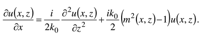
In equation (1) k0 is the free-space wave number, m=M10-6+1 is the modified refractive index, u(x,z) is the reduced function [34], obtained by factoring out the rapid fluctuations of the electromagnetic (EM) field component, x and z stay for range and altitude. This parabolic approximation of the wave equation is easily solved numerically by means of marching algorithms provided the electromagnetic field is known on an initial plane and respective boundary conditions are available. The limitations of the 2D PE and its numerical solutions are discussed in [37, 44, 45]. In this study (1) is solved using the split-step Fourier-transform (SSF) solution as described and implemented in "Advanced propagation model (APM) version 1.3.1 Computer software configuration item (CSCI) documents", Tech. Doc. 3145, see [45]. The output of the PE model is obtained in terms of path loss (PL, PL in dB) or propagation factor (PF, PF in dB) calculated following (2):
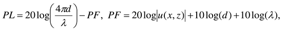 where λ is the free-space wavelength, d is the distance between the corresponding points and the first term in the right-hand side of the expression for the PL is the free-space loss. Here the PF is defined as PF=|E/E0|2, where E is the electric field amplitude received at a given point under specific conditions and E0 is the electric field amplitude received in the same point under free-space conditions [12]. This definition of the PF accounts for all propagation effects, including multipath and diffraction, between the two corresponding points as well as the transmitter antenna pattern.
In this study the initial field needed to start the calculations is provided by an omni directional antenna. A trans-horizon path supposes multiple reflections from the sea surface; therefore the sea surface roughness should be accounted for. A good indicator of the surface roughness is the Rayleigh roughness parameter 2k0σhsin(α) [34], where σh is the standard deviation of the sea surface height and α is the grazing incidence angle to the surface; i.e. the degree of roughness is determined not only by σh but also by the radio frequency and angle of incidence α. Two international channels in the VHF maritime mobile band centered at 161.975 MHz and 162.025 MHz are allocated to the AIS which correspond to wavelength of about 1.85 m, i.e. it is of the same order as sea height variations in high sea states. On the other hand, the ducting propagation and ship-to-ship communication imply small grazing angles which reduce the influence of roughness. The significance of sea surface roughness for AIS frequencies is still an open issue that is beyond the scope of this work. In this study the sea surface is considered as smooth and Fresnel reflection coefficient from smooth surface is applied to account for the sea surface reflection. The dielectric characteristics of the sea water are calculated as functions of frequency following [27]. The environmental input to the PE is provided by M profiles taken from [46], see Figures 2, 3, and 5 of the Results and Discussion section below.
2.2. Troposcatter model
At ranges sufficiently greater than the radio horizon when there are no trapping layers and ducting, the scattering from irregularities in the troposphere becomes the dominant propagation mechanism. The troposcatter model used in this work follows that described in [25]. The median path loss in the troposcattering region, with the free-space loss included, is given by:
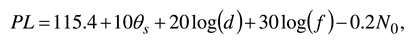
where θs is the scattering angle in degrees, see Figure 2, d is the ground range between the transmitter and receiver in km, f is the frequency in MHz, and N0 (N-units), the sea-level surface refractivity, which is a measure of location variability of the troposcatter mechanism. For a smooth earth the scattering angle is:
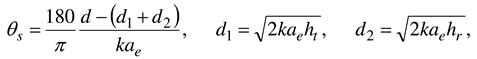
where ht, hr, are the transmitter and receiver heights, ae=6370 km is the Earth radius, k is the effective earth radius factor. For standard refractivity conditions where dN/dz = -39 N-units per kilometer (dM/dz = 118 M-units per kilometer), k = 1.3333 or four-thirds.
It is difficult to strictly distinguish the range of application between the diffraction propagation mechanism, calculated by PE, and troposcatter mechanism where (3) applies. Here as a criterion is used the minimum range rd at which the diffraction solution is applicable [47]:
where rhor is the horizon range, rhor is in km, ht, hr are in meters, f in MHz. The troposcatter model (3) is used for all range-height combinations beyond rd in parallel with the PE model which provides the losses from the other propagation mechanisms (standard troposphere, diffraction, reflection). It should be noted that another approach, aimed at modeling turbulence effects from higher altitudes again using PE, is implemented in [48] where a semi-empirical scatter model adds a random fluctuation to the mean refractive-index value at each height considered by the parabolic equation method. This approach is attractive, but a number of concerns associated with it that may affect the general application of the PE are also discussed in [48].
It is to note that in (3) is missing the aperture-to-medium coupling loss factor which accounts for the common volume variation with antenna gain and has been added later to the troposcatter loss model [5, 27, 29]. Since the present study uses omni directional antenna the aperture-to-medium coupling loss factor is effectively zero. Contrary, because the frequency is relatively low and lower antenna heights are used, the original formula (3) is complemented by the frequency-gain function H0 as described and derived in [26]. For lower frequencies the effective antenna heights ht/λ and hr/λ in wavelengths become smaller, and ground-reflected energy tends to cancel direct-ray energy at the lower part of the common volume, where scattering efficiency is greatest.
3. Results and discussion
The examples of M profiles, used as environmental input to the PE in this study, are shown in Figures 3, 4, and 5. They are selected from among the profiles obtained in [46] where the M profiles are calculated from meteorological parameters provided by ECMWF for the Bulgarian Black sea shore for a period of two years. The number and heights of the linear segments that approximate the M profiles correspond to the levels at which the meteorological parameters were available. The exact latitude and longitude are indicated inside the pictures with the date to which the profiles refer. In Figure 3 and Figure 4 profiles named as “first” are at a distance of about 25 km from the shore, profiles said “second” are at a distance of about 50 km going far out to the sea. Figure 3 presents increase of the thickness of a surface-based duct (SBD) from the shore to the open sea; Figure 4 shows evolution of profiles from the shore to the open sea leading to formation of an elevated duct. On Figure 5 is shown the averaged surface duct profile for summer months at the shore (43°N–28°E) from the above study as well as a log-linear evaporation duct profile with zd=40 m following [13] (evaporation ducts are not included in [46]):
 where z0 is the aerodynamic roughness parameter assumed to be 1.5x10⁻⁴ m [13, 34].
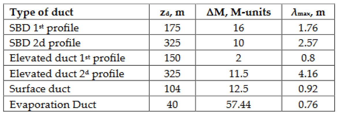
In order to preliminary assess the trapping of the AIS frequencies, well known formula for maximum wave length, λmax, trapped in a duct is often used [49]:
where zd is the duct thickness, ∆M is the M-deficit, see Figure 1, and C=3.77x10⁻³ for surface and surface-based ducts and C =5.66 x 10⁻³ for elevated ducts. It indicates that the evaporation duct is not able to trap the AIS frequencies with its maximal height of 40 m and M-deficit determined by the most widely used log-linear approximation of its average M profile, (6), see Table 1. Indeed, as it is seen from Table 1, only the second SBD and second elevated duct profiles assure, according to (7), the full trapping of AIS frequencies. It is to note that the transition from ducting to non-ducting conditions (and vice versa) for frequencies with λ around λmax is gradual and those frequencies can be affected by the duct even though not (fully) trapped. In all subsequent calculations the frequency F=161.975 MHz is used. If not indicated, horizontal polarization is applied.
In Figure 6 and Figure 7 are compared the PL curves vs range for the two SBDs from Figure 3 and the respective troposcatter curves, (3), calculated for the values of M0 corresponding to those of the SBDs. The troposcatter curves are complemented by the standard troposphere and diffraction PL. Figure 8 and Figure 9 show analogous results but for the two elevated ducts from Figure 4. The other parameters are: ht=25 m, hr=30 m for Figure 6 and Figure 8; ht=55 m, hr=30 m for Figure 7 and Figure 9. As expected, the ducting assures less PL than troposcatter, especially for beyond 100 km region, even when λmax is less then 1.85 m. Beyond-the-horizon regions (rhor= 43 km for Figure 6 and Figure 8; rhor= 53 km for Figure 7 and Figure 9) are characterized by smooth PL increase in the case of SBDs and PL peaks that exceed the troposcatter values (or those of standard troposphere plus diffraction, if the range is less than rd) for the elevated ducts. For the elevated ducts and used ht, for lower (receive) antennas a “skip zone” exits beyond 40 km, see Figure 10 when the PL is plotted vs range and height for ht=25 m. In this figure, the locations of the two PL peaks for the second elevated duct from Figure 8 near range=50 km and range=92 km are clearly visible. Figure 11 shows PL vs range and height for the second SBD and ht=25 m. The SBDs are formed with the participation of elevated trapping layers; those layers “pull” the energy upwards and a skip zone is formed close to the earth surface; see also [10, 50]. In comparison to the elevated duct, in the case of SBD the skip zone does not show PL peaks, they are “diffused”, but in the first 30-40 m (for this specific case) the loss is higher than the above. In Figure 6 (ht=25 m) the weaker SBD has less PL than the stronger one, but in Figure 7 where ht=55 m the situation is as expected: the stronger duct leads to less PL than the weaker duct. In the maritime communications, the elevated ducts have been considered to have weak influence due to there relatively great height above the sea surface [51]. Indeed, the elevated ducts from Figure 4 result in higher PL than the SBDs from Figure 3, but more importantly, the presence of elevated trapping layers forming elevated ducts perturbs the propagation "pattern" in the lower tens of meters above the sea. Note also that the two ducts from the SBD pair coexisted separated by a distance of 25 km; the same applies to the pair of elevated ducts. The range-dependent ducting for AIS frequencies is studied in [52]; here results are given for only the four characteristic duct types. In Figure 8 and Figure 9 the different values of M0 lead to a slight difference in troposcatter, whereas in Figure 6 and Figure 7 the two troposcatter curves overlap because the two M0 value are too close.
In Figure 12 are compared the PL curves vs range for the surface duct from Figure 5 for two transmitter heights, ht=25 m and ht=55 m, and the respective troposcatter curves, (3). The receiver height is hr=30 m; in this figure is seen the influence of the ht on the troposcatter which is rather negligible, see also [5]. Here again, although the AIS frequency is not well trapped, the ducting assures significantly less PL than troposcatter. Figure 13 shows PL vs range and height for the surface duct and ht=25 m; the PL increases smoothly with height and range. In the case of surface duct it seems that the general rule “the higher the antenna the lower the PL” is still valid.
Figure 14 shows the PL curves for evaporation duct (with parameters from Table 1), troposcatter, and standard troposphere for ht=55 m, hr=30 m. Compared to the standard troposphere, in the region beyond the horizon the PL is reduced by about 10 dB due to the evaporation duct. Note that after about 140 km, the troposcatter PL is less than that of evaporation duct.
Figure 15 compares the troposcatter for AIS from [5] for ht=10 m, hr=50 m, and that calculated by (3) with the same ht, hr. Two curves are generated by (3): one applies the maximum M0=383 M-units, the other the minimum M0=333 M-units used in this study. The troposcatter PL calculated by (3) falls between losses not exceeded for 50% of time and those not exceeded for 99% of time. The difference in PL determined by the two M0 values can reach 10 dB with troposcatter model (3).
4. Conclusion
This work presents results on the comparison between the PL due to troposphere ducting and PL due to troposcatter for the AIS frequencies. These two beyond LoS propagation mechanisms are assessed using the PE method in which a simple troposcatter formula is incorporated. The simulations have shown that the ducting assures significantly greater reduction of PL than troposcatter and this is valid even when the AIS frequencies are not well trapped in the duct; the evaporation duct is an exception of this “rule”. Although they are located high above the area of interest, the elevated trapping layers should not be underestimated; it appears that the elevated ducts formed by those layers create more inhomogeneous propagation environment in the first tens meters (and beyond) above the sea surface. Special attention should be paid to the skip zones; in their presence the ducting propagation can lose its advantage. Among the different duct types, surface and surface-based ducts appear as the major candidate to contribute to the increase of the AIS detection range. Those ducts provide a smooth increase in PL with range and height; in addition, they are less sensitive to frequency than evaporation ducts, can extend over the ocean for several hundreds of kilometers, and last for multiple days.
This duct-troposcatter comparison can be seen as a preliminary estimate that should be further improved by a more complex troposcatter formulation and the introduction of sea surface roughness for both propagation mechanisms. It should be emphasized that whatever complex radio wave propagation method is used, it is based on the environmental data that serve as its input. Thus the good knowledge of (local and not only) environmental characteristics as availability of irregularities in the troposphere, duct types and their statistics, presence of M profiles with multiple inversions or range-dependency (not included in this study), will make the prediction of the possible increase of the AIS detection range more reliable and of practical use. Also, this means that the coastal equipment must be able to evaluate both of these and, possibly, others beyond LoS propagation mechanisms.
Funding
This research was funded by the Ministry of Education and Science of Bulgaria (support for ACTRIS BG, part of the Bulgarian National Roadmap for Research Infrastructure).
Conflicts of Interest
The author declare no conflict of interest.
References
- International Telecommunication Union. R-REC-M.2092-1: Technical characteristics for a VHF data exchange system in the VHF maritime mobile band; Electronic Publication: Geneva, Switzerland, 2022.
- Jiang, S. Networking in ocean: a survey. ACM Computing Surveys 2022, 54, 13:1-13:33.
- Wright, D.; Janzen, C.; Bochenek, R.; Austin, J.; Page, E. Marine Observing applications using AIS: Automatic Identification System. Front. Mar. Sci. 2019, 6. [CrossRef]
- Emmens, T.; Amrit, C.; Abdi, A.; Ghosh, M. The promises and perils of Automatic Identification System data. Expert Sys. Appl. 2021, 178. [CrossRef]
- International Telecommunication Union. ITU-R M.2123: Long range detection of automatic identification system (AIS) messages under various tropospheric propagation conditions; ITU: Geneva, Switzerland, 2007.
- Dinc, E.; Akan, O. B. Beyond-line-of-sight communications with ducting layer. IEEE Commun. Mag. 2014, 52, 37–43. [CrossRef]
- Tang, W.; Cha, H.; Wei, M.; Tian. B. Estimation of surface-based duct parameters from automatic identification system using the Levy flight quantum-behaved particle swarm optimization algorithm. JEWA 2019, 33, 827-837. [CrossRef]
- Tang, W.; Cha, H.; Wei, M.; Tian, B.; Li, Y. A Study on the Propagation Characteristics of AIS Signals in the Evaporation Duct Environment. ACES Journal 2019, 34, 996-1001.
- Robinson, L.; Newe, T.; Burke, J.; Toal, D. A simulated and experimental analysis of evaporation duct effects on microwave communications in the Irish Sea. IEEE Trans. on AP 2022, 70, 4728–4737. [CrossRef]
- Shi, Y.; Wang, S.; Yang, F.; Yang, K. Statistical analysis of hybrid atmospheric ducts over the Northern South China sea and their influence on over-the-horizon electromagnetic wave propagation. J. Mar. Sci. Eng. 2023, 11, 669. [CrossRef]
- Bastos, L.; Wietgrefe, H. A Geographical analysis of highly deployable troposcatter systems performance. In Proceeding of the 2013 IEEE Military Communications Conference, San Diego, CA, USA, 18-20 November 2013; pp. 661-667. [CrossRef]
- Propagation of Short Radio Waves, 2nd ed.; Kerr, D.E., Ed.; Peter Peregrinus: London, UK, 1987.
- Paulus, R.A. Practical application of an evaporation duct model. Radio Sci. 1985, 20, 887–896. [CrossRef]
- Yang, C.; Shi, Y.; Wang J.; Feng, F. Regional spatiotemporal statistical database of evaporation ducts over the South China Sea for future long-range radio application. IEEE J. Sel. Top. Appl. Earth Obs. Remote Sens. 2022, 15, 6432-6444. [CrossRef]
- Yang, N.; Su, D.; Wang, T. Atmospheric ducts and their electromagnetic propagation characteristics in the Northwestern South China Sea. Remote Sens. 2023, 15, 3317. [CrossRef]
- Rautiainen, L.; Tyynelä, J.; Lensu, M.; Siiriä, S.; Vakkari, V.; O’Connor, E.; Hämäläinen, K.; Lonka, H.; Stenbäck, K.; Koistinen, J.; et al. Utö observatory for analysing atmospheric ducting events over Baltic coastal and marine waters. Remote Sens. 2023, 15, 2989. [CrossRef]
- von Engeln A.; Teixeira J., A ducting climatology derived from ECMWF global analysis fields. J Geophys. Res. 2004, 109. doi:10.1029/2003JD004380.
- Yang, C.; Wang, J. The investigation of cooperation diversity for communication exploiting evaporation ducts in the South China Sea. IEEE Trans. on AP 2022, 70, 8337-8347. [CrossRef]
- Zaidi, K.S.; Hina, S.; Jawad M.; Khan, A.N.; Khan, M.U.S.; Pervaiz, H.B.; Nawaz, R. Beyond the horizon, backhaul connectivity for offshore IoT devices. Energies 2021, 14, 6918. [CrossRef]
- Ma, J; Wang, J.; Yang, C. Long-range microwave links guided by evaporation ducts. IEEE Commun. Mag. 2022, 60, 68-72. [CrossRef]
- Sirkova, I. Anomalous tropospheric propagation: usage possibilities and limitations in radar and wireless communications systems. In: Proceedings of the 10th Jubilee International Conference of the Balkan Physical Union, Sofia, Bulgaria, 26-30 August, 2018. [CrossRef]
- Valčić, S.; Brčić, D. On detection of anomalous VHF propagation over the Adriatic Sea utilizing a software-defined Automatic Identification System receiver. J. Mar. Sci. Eng. 2023, 11, 1170. [CrossRef]
- Huang, L.-F.; Liu, C.-G.; Wu, Z.-P.; Zhang, L.-J.; Wang, H.-G.; Zhu, Q.-L.; Han, J.; Sun, M.-C. Comparative analysis of intelligent optimization algorithms for atmospheric duct inversion using Automatic Identification System signals", Remote Sens. 2023, 15, 3577. [CrossRef]
- Han, J.; Wu, J.; Zhang, L.; Wang, H.; Zhu, Q.; Zhang, C.; Zhao, H.; Zhang, S. A Classifying-inversion method of offshore atmospheric duct parameters using AIS data based on artificial intelligence. Remote Sens. 2022, 14, 3197. [CrossRef]
- Yeh, L. Simple methods for designing troposcatter circuits. IRE Trans. Commun. Syst. 1960, 8, 193-198. [CrossRef]
- Rice, P.L.; Longley, A.G.; Norton, K.A.; Barsis, A.P. Transmission Loss Predictions for Tropospheric Communication Circuits; Department of Commerce, National Bureau of Standards: Maryland, US, 1965.
- International Radio Consultative Committee. Recommendations and Reports of the CCIR: Propagation in non-ionized media; CCIR: Geneva, Switzerland, 1986.
- International Telecommunication Union. Recommendation ITU-R P.452-16: Prediction procedure for the evaluation of interference between stations on the surface of the Earth at frequencies above about 0.1 GHz; Electronic Publication: Geneva, Switzerland, 2015.
- International Telecommunication Union. Recommendation ITU-R P.617-2: Propagation prediction techniques and data required for the design of trans-horizon radio-relay systems; Electronic Publication: Geneva, Switzerland, 2012.
- International Telecommunication Union. Recommendation ITU-R P.2001-3: A general purpose wide-range terrestrial propagation model in the frequency range 30 MHz to 50 GHz; Electronic Publication: Geneva, Switzerland, 2019.
- Li, L.; Wu, Z.-S.; Lin, L.-K.; Zhang, R.; Zhao, Z.-W. Study on the prediction of troposcatter transmission loss. IEEE Trans. on AP 2016, 64, 1071-1079. [CrossRef]
- Yuan, D.; Chen, X. Troposcatter transmission loss prediction based on particle swarm optimization. IET Microw. 2021, 15, 332-341. [CrossRef]
- Lee, I.-S.; Noh, J.-H.; Oh, S.-J. A Survey and analysis on a troposcatter propagation model based on ITU-R recommendations. ICT Express 2023, 9, 507-516. [CrossRef]
- Levy, M. Parabolic Equation Methods for Electromagnetic Wave Propagation; IEE: London, UK, 2000.
- Kuttler, J.R.; Dockery, G.D. Theoretical description of the parabolic approximation Fourier split-step method of representing electromagnetic propagation in the troposphere. Radio Sci. 1991, 26, 381–393. [CrossRef]
- Apaydin, G.; Sevgi, L. Radio Wave Propagation and Parabolic Equation Modeling; Wiley-IEEE Press: Hoboken, New Jersey, US, 2017.
- Sirkova, I. Brief review on PE method application to propagation channel modeling in sea environment. CEJE 2012, 2, 19-38. [CrossRef]
- Zhang, P.; Bai, L.; Wu, Z.; Guo, L. Applying the parabolic equation to tropospheric groundwave propagation: a review of recent achievements and significant milestones. IEEE Antennas Propag. Mag. 2016, 58, 31–44. [CrossRef]
- Apaydin, G.; Sevgi, L. The split-step-Fourier and finite-element based parabolic-equation propagation prediction tools: canonical tests, systematic comparisons, and calibration. IEEE Antennas Propag. Mag. 2010, 52, 66–79. [CrossRef]
- Barrios, A.E.; Anderson, K.; Lindem, G. Low altitude propagation effects - a validation study of the Advanced Propagation Model (APM) for mobile radio applications. IEEE Trans. on AP 2006, 54, 2869-2877. [CrossRef]
- Gunashekar, S.D.; Warrington, E.M.; Siddle D.R.; Valtr P. Signal strength variations at 2 GHz for three sea paths in the British Channel islands: detailed discussion and propagation modeling. Radio Sci. 2007, 42, doi:10.1029/2006RS003617.
- Heemskerk, E. RF propagation measurement and model validation during RF/IR synergy trial VAMPIRA. In: Proceedings of SPIE Remote Sensing: Optics in atmospheric propagation and adaptive systems VIII, Bruges, Belgium, 20-21 September 2005; pp. 598107.1-598107.12. [CrossRef]
- Wang, Q.; Alappattu, D.P.; Billingsley, S.; Blomquist, B.; Burkholder, R.J. et al. CASPER: coupled air-sea process and electromagnetic wave ducting research. Bull. Amer. Meteor. Soc. 2018, 99, 1449–1471. [CrossRef]
- Wang, J.; Zhou, H.; Li, Y.; Sun, Q.; Wu, Y.; Jin, S.; Quek, T.Q.S.; Xu, C. Wireless channel models for maritime communications. IEEE Access 2018, 6, 68070-68088. [CrossRef]
- Barrios, A. E. Considerations in the development of the advanced propagation model (APM) for U.S. navy applications. In Proceedings of the International Conference on Radar (IEEE Cat. No.03EX695), Adelaide, SA, Australia, 3-5 September 2003; pp. 77-82. [CrossRef]
- Sirkova, I. Duct occurrence and characteristics for Bulgarian Black sea shore derived from ECMWF data. J. Atmos. Sol-Terr. PHy. 2015, 135, 107-117. [CrossRef]
- Reed, H.R.; Russell, C.M. Ultra high frequency propagation; Boston Technical Publishers: Cambridge, US, 1966.
- Hitney, H.V. A practical tropospheric scatter model using the parabolic equation. IEEE Trans. on AP 1993, 41, 905-909. [CrossRef]
- Turton, J.D.; Bennetts, D.A.; Farmer, S.F.G. An introduction to radio ducting. Meterorolog. Mag. 1988, 117, 245-254.
- Rol, M.; Nijboer, R.; Yarovoy, A. Radio wave blind zone in a duct: an analytical approach. In Proceeding of the 24th International Microwave and Radar Conference (MIKON), Gdansk, Poland, 12-14 September, 2022; pp. 1-6. [CrossRef]
- D. Couillard, G. Dahman, M. GrandMaison, G. Poitau and F. Gagnon, Robust broadband maritime communications: theoretical and experimental validation. Radio Sci. 2018, 53, 749-760. [CrossRef]
- Sirkova, I. Automatic Identification System Signals propagation in troposphere ducting conditions. In Proceedings of the 10th IEEE International Black Sea Conference on Communications and Networking (BlackSeaCom), 6-9 June 2022, Sofia, Bulgaria; pp. 331-335. [CrossRef]
Figure 1.
M(z) profiles for: (a) evaporation duct; (b) surface duct; (c) surface-based duct; (d) elevated duct.
Figure 1.
M(z) profiles for: (a) evaporation duct; (b) surface duct; (c) surface-based duct; (d) elevated duct.
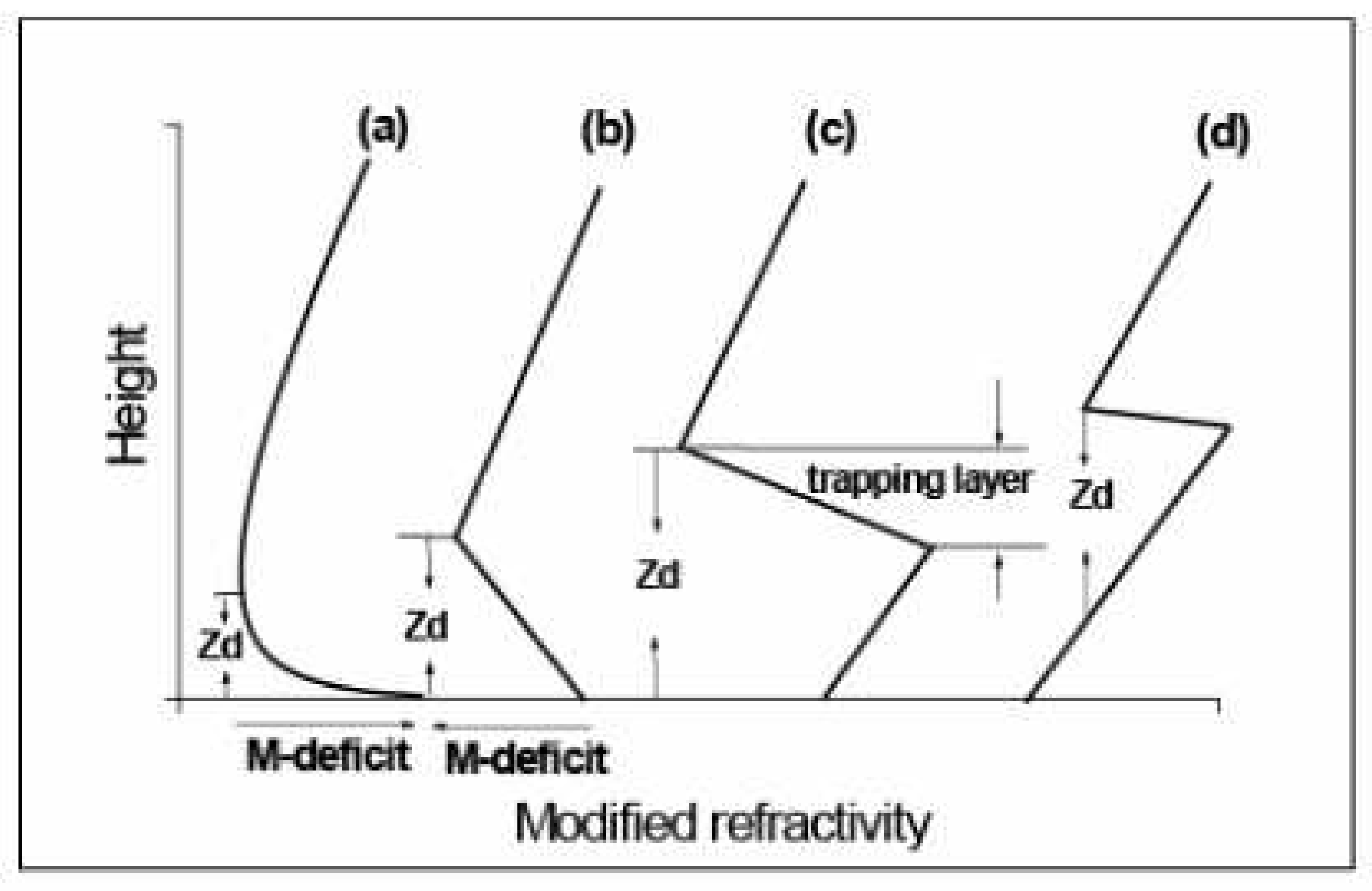
Figure 2.
The geometry of the troposcatter model.
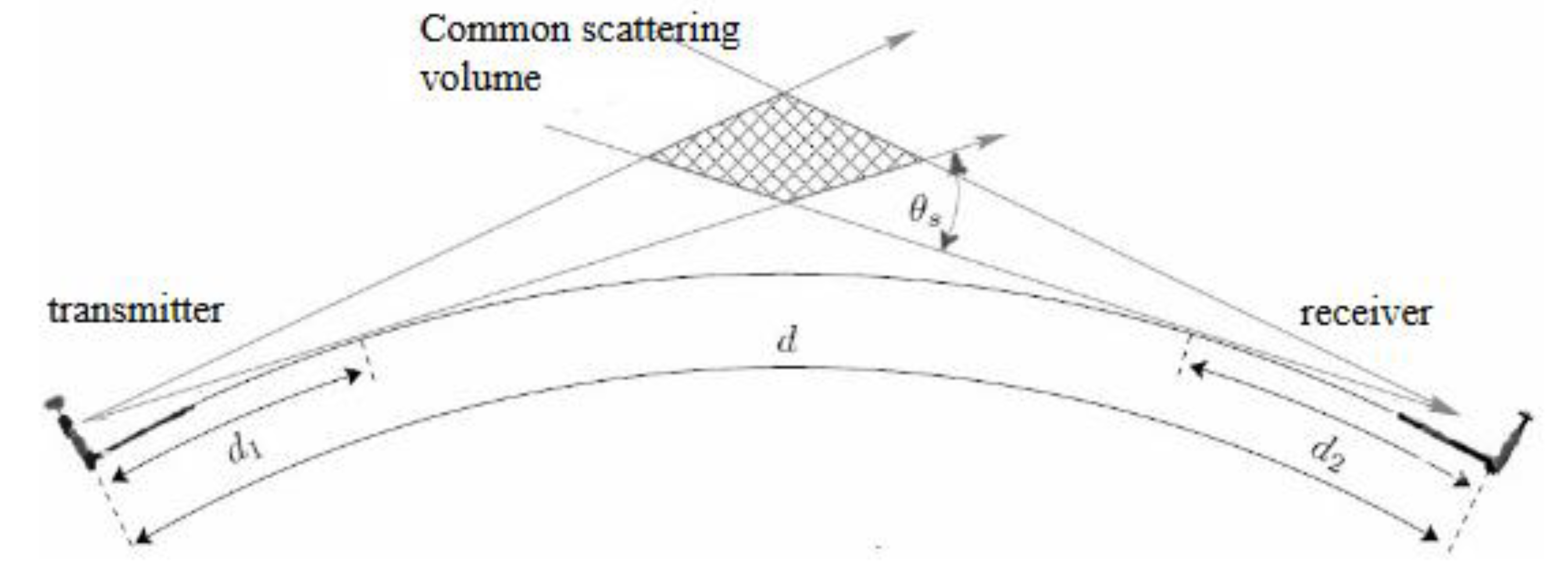
Figure 3.
Surface-based ducts profiles.
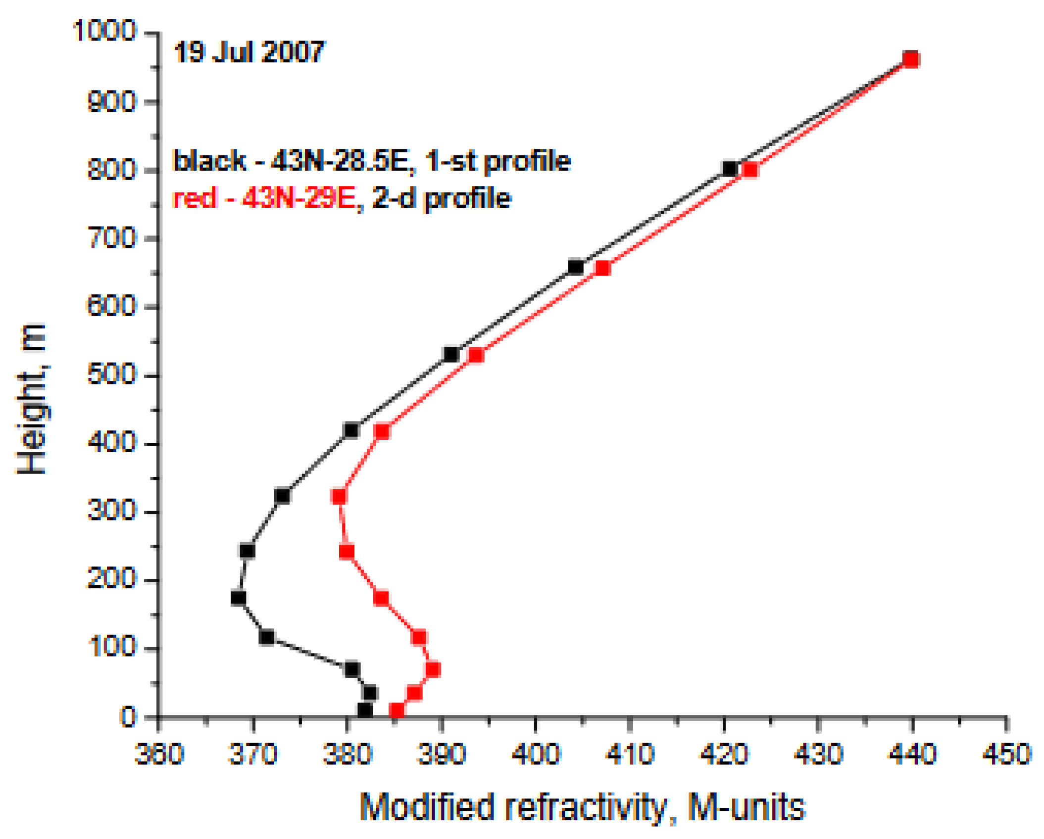
Figure 4.
Elevated ducts profiles.
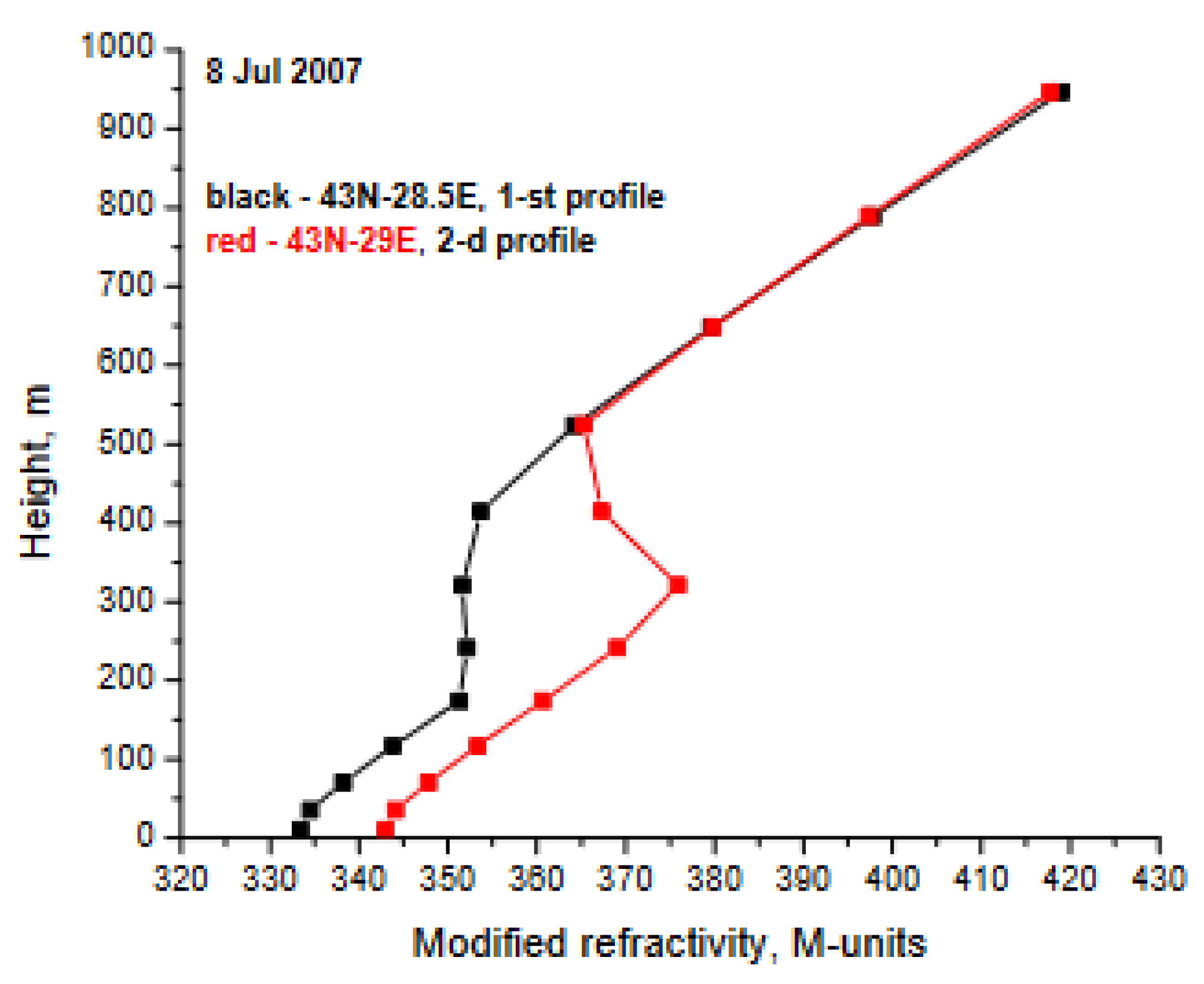
Figure 5.
Evaporation duct profile (a), surface duct profile (b).
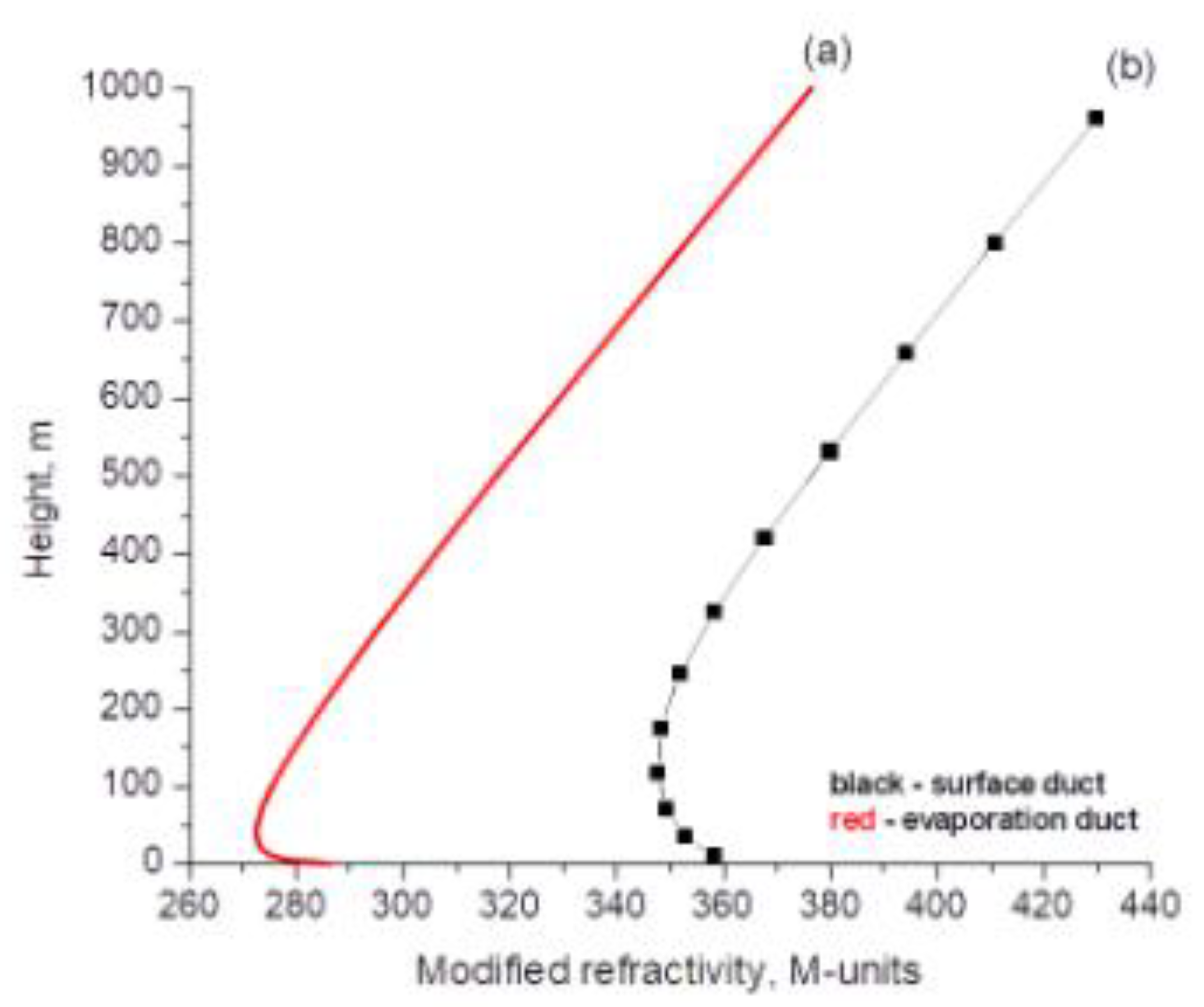
Figure 6.
PL for SBDs and troposcatter,ht=25 m, hr=30 m.
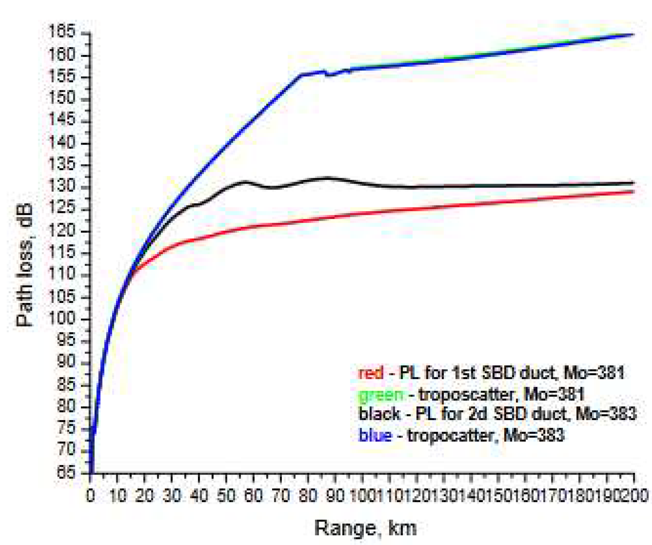
Figure 7.
PL for SBDs and troposcatter, ht=55 m, hr=30 m
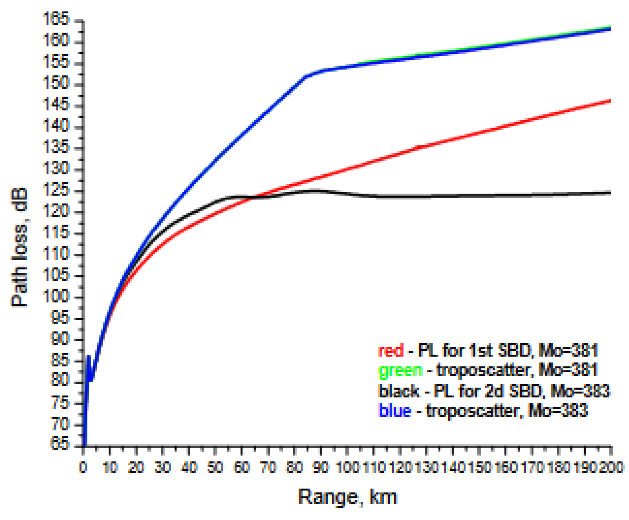
Figure 8.
PL for elevated ducts and troposcatter, 25 m, .hr=30 m.
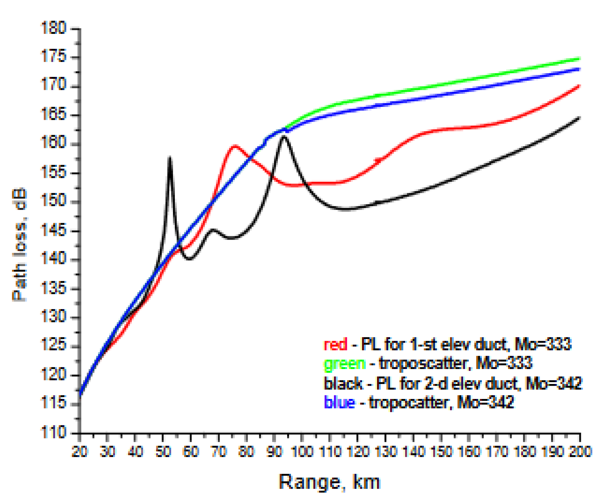
Figure 9.
PL for elevated ducts and ht=55 m, hr=30 m.
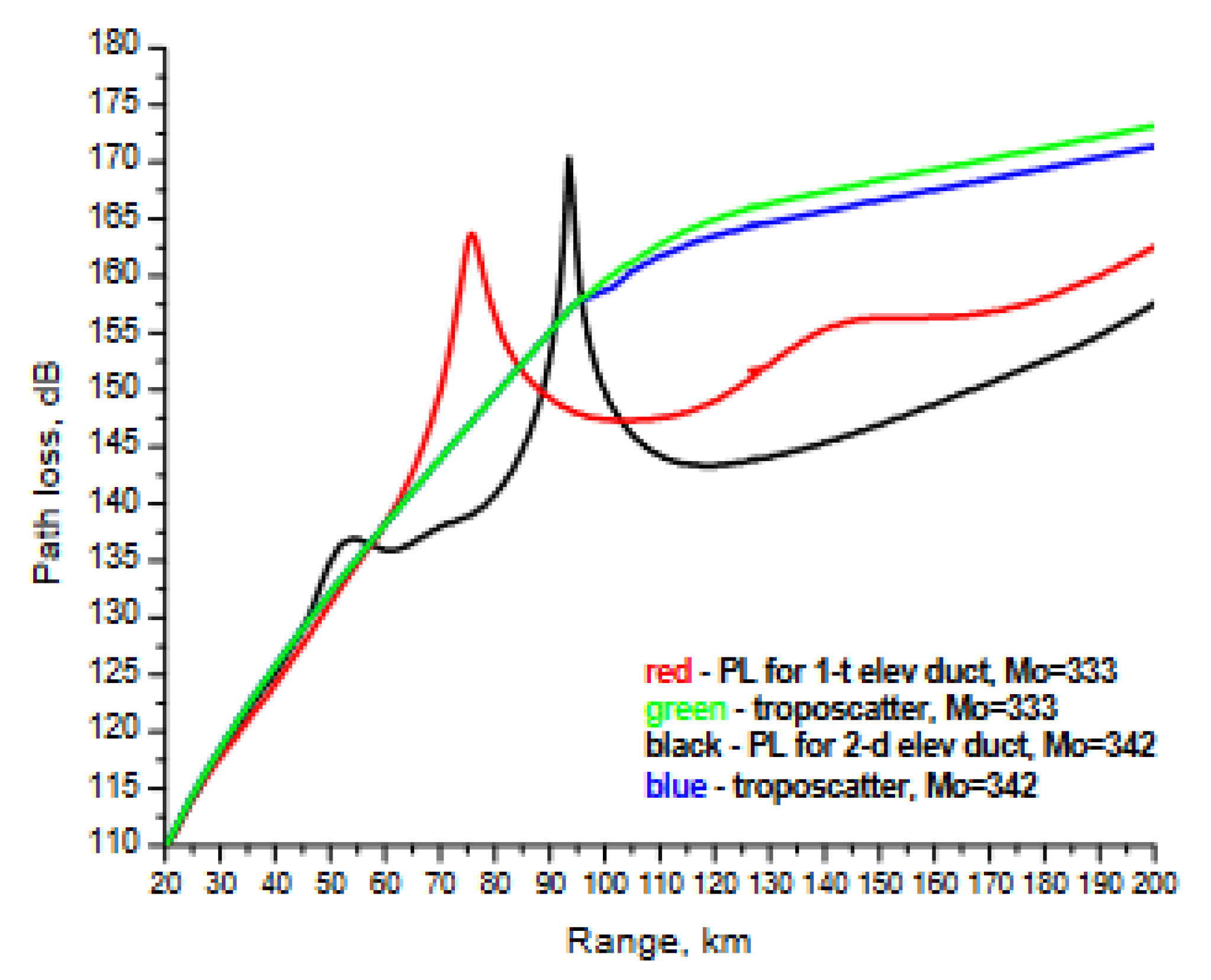
Figure 10.
Coverage diagram for the second elevated duct, ht=25 m.
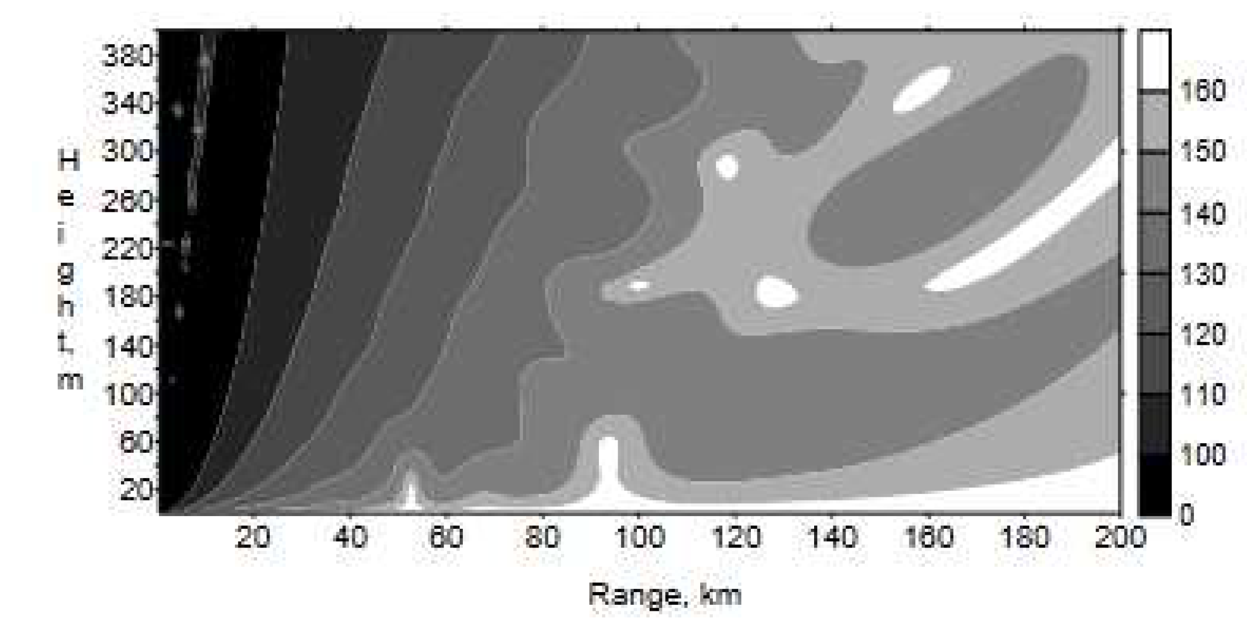
Figure 11.
Coverage diagram for the second surface-based duct, ht=25 m.
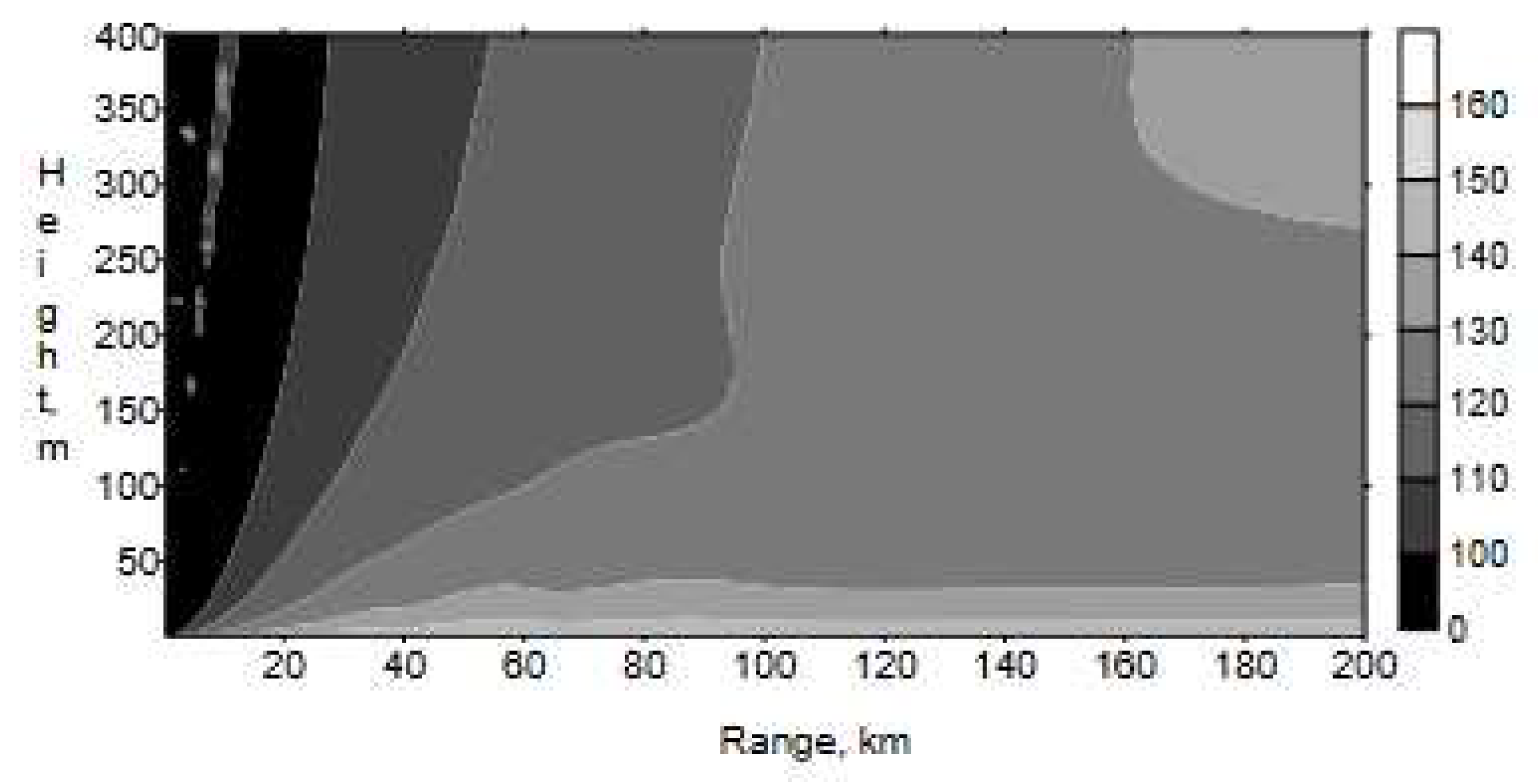
Figure 12.
PL for surface duct and troposcatter for ht=25 m and ht =55 m.
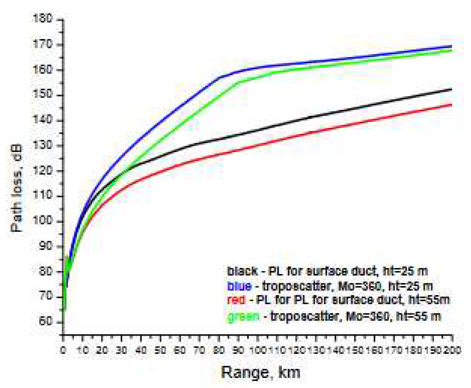
Figure 13.
Coverage diagram for the surface duct, ht =25 m.
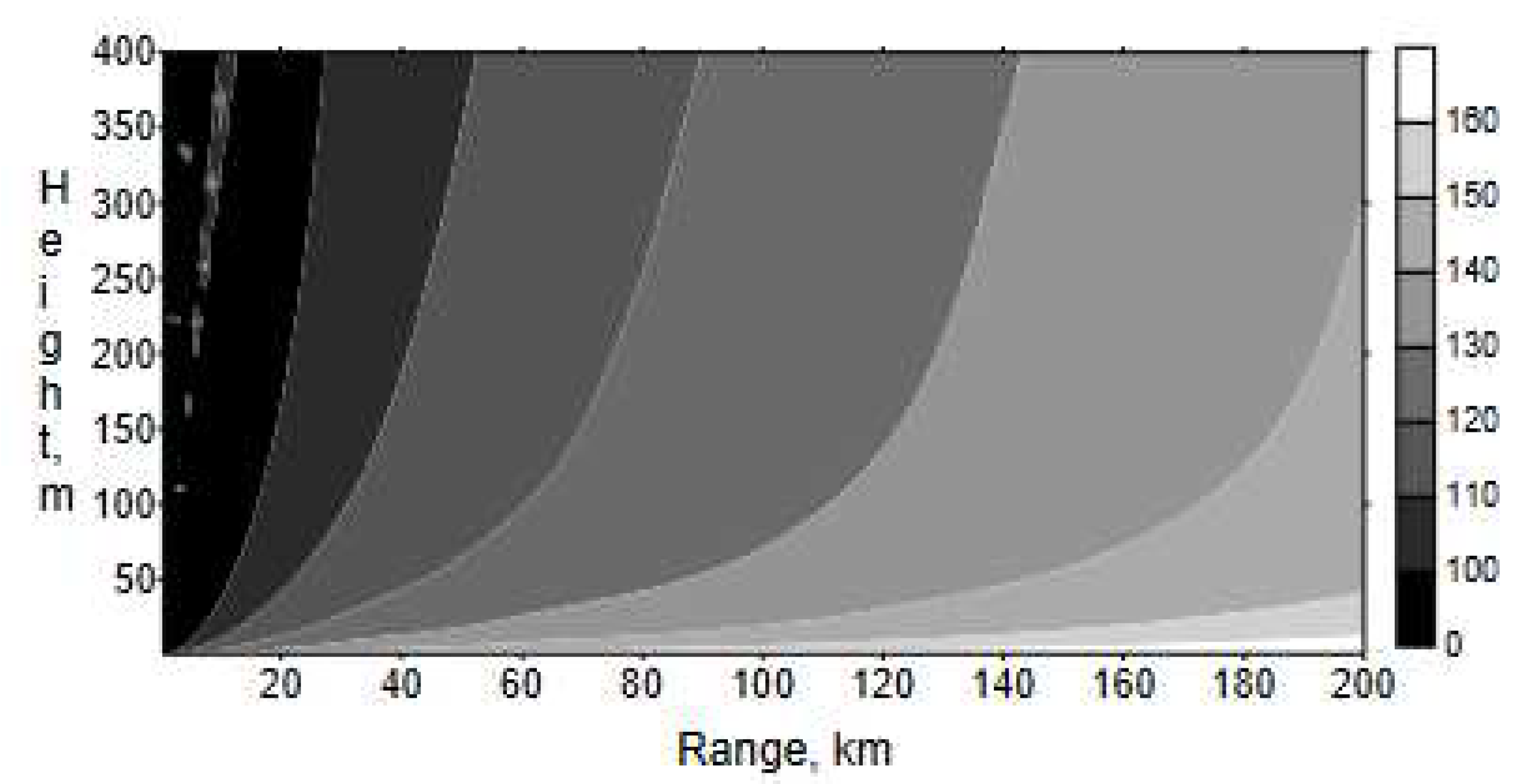
Figure 14.
PL for evaporation duct, standard troposphere and troposcatter, ht =55 m.
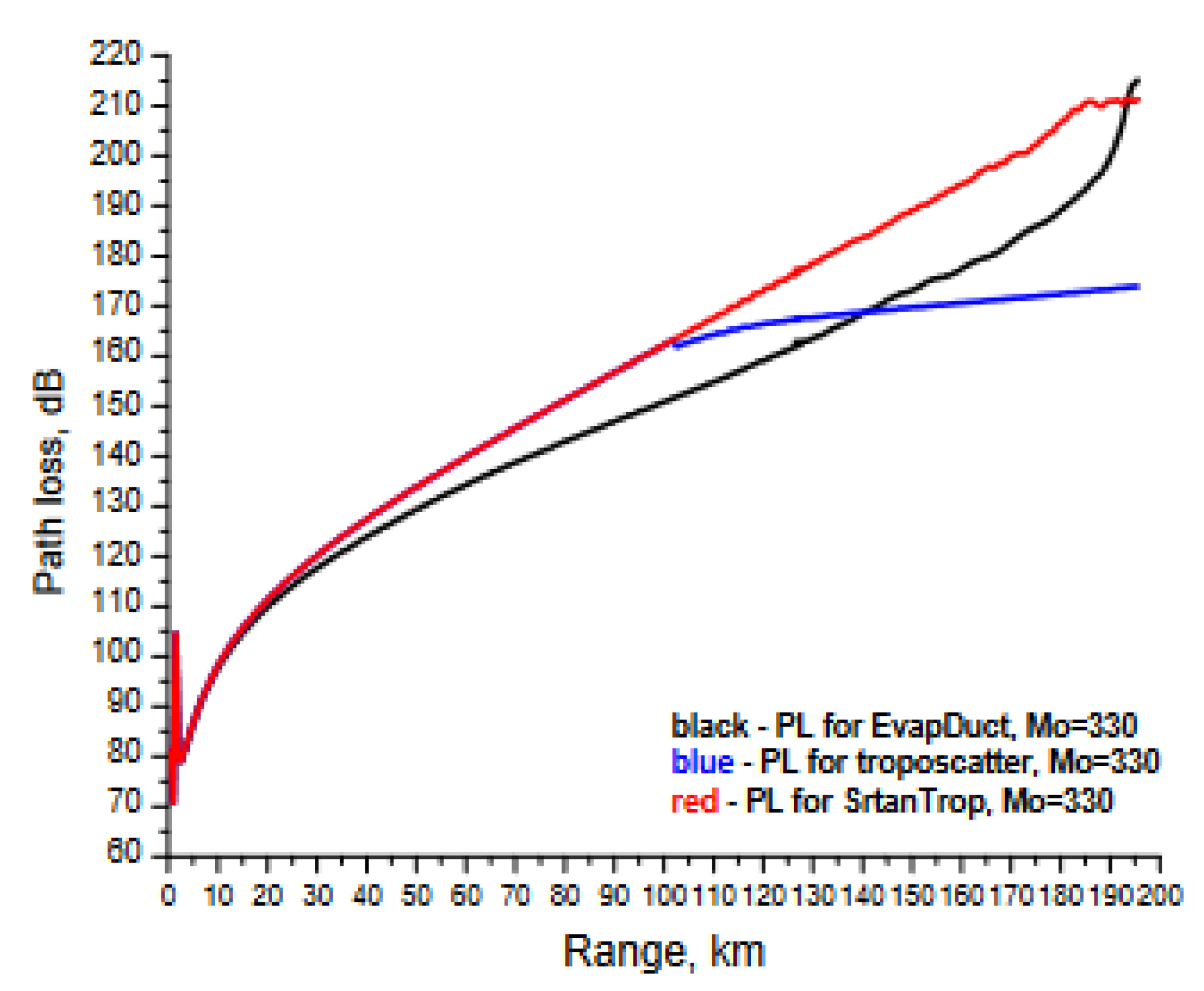
Figure 15.
Comparison between troposcatter from (3) and [5].
Figure 15.
Comparison between troposcatter from (3) and [5].
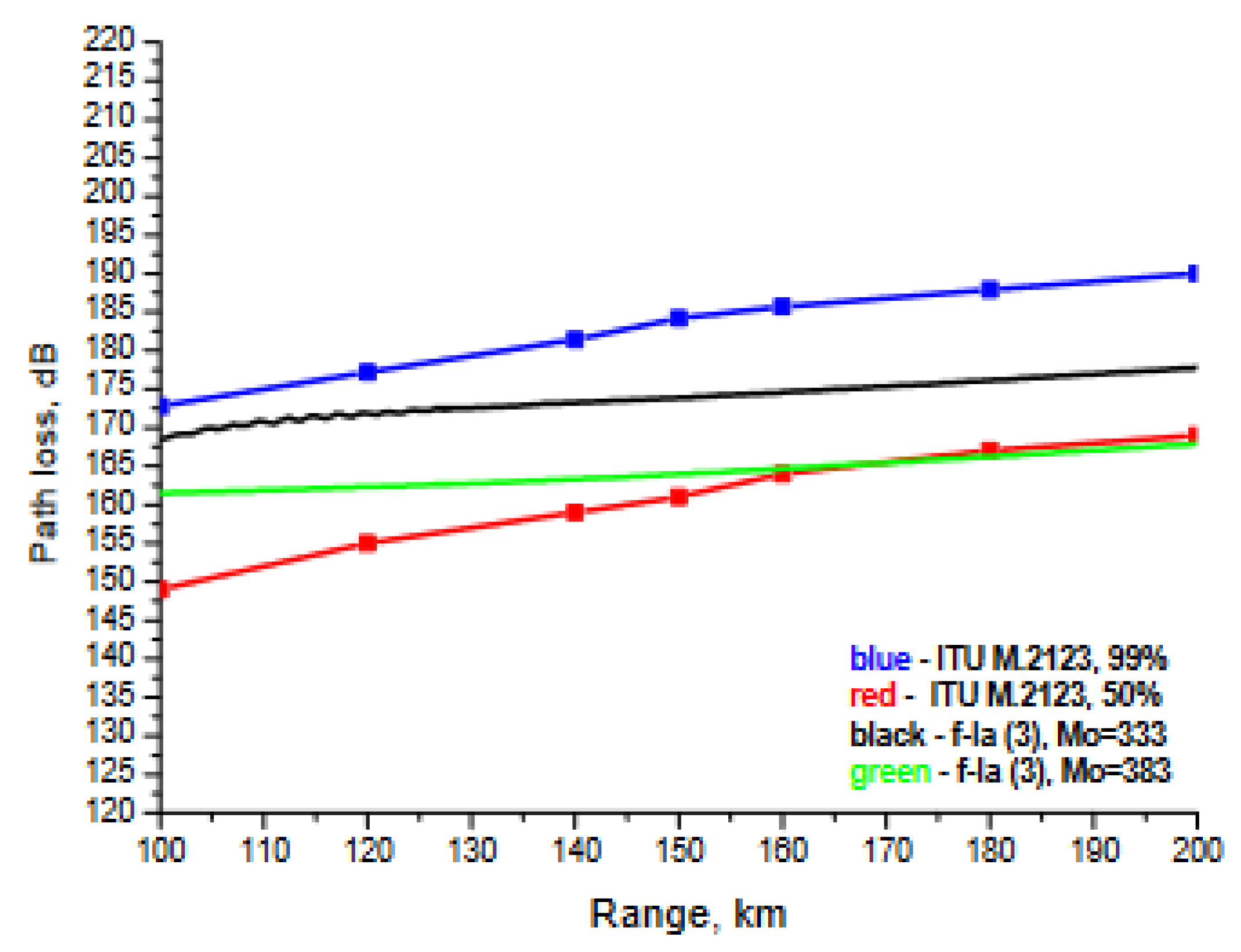

Table 1.
Essential duct parameters for ducts in Figures 3, 4, and 5.
 |
Disclaimer/Publisher’s Note: The statements, opinions and data contained in all publications are solely those of the individual author(s) and contributor(s) and not of MDPI and/or the editor(s). MDPI and/or the editor(s) disclaim responsibility for any injury to people or property resulting from any ideas, methods, instructions or products referred to in the content. |
© 2023 by the authors. Licensee MDPI, Basel, Switzerland. This article is an open access article distributed under the terms and conditions of the Creative Commons Attribution (CC BY) license (http://creativecommons.org/licenses/by/4.0/).
Copyright: This open access article is published under a Creative Commons CC BY 4.0 license, which permit the free download, distribution, and reuse, provided that the author and preprint are cited in any reuse.


