Submitted:
22 August 2023
Posted:
24 August 2023
You are already at the latest version
Abstract
The study presented here, through the use of GIS and physical variables, generate a new meth-odology for the calculation of erosivity (Factor R) for the qualitative evaluation of soil loss po-tential (laminar erosion) in the Northwest margin of the municipality of São Francisco, mostly located in the Pardo-MG river basin. The results obtained were statistically correct when com-pared to the traditional R calculation and the laminar erosion methodology. It is worth noting that the new proposal presented here indicated sites of qualitative loss of soil in the same places where there are closed-loop satellite signals of degraded Cerrado, something not identified in the traditional model. As conclusion it can be said that the obtained results were extremely sat-isfactory, being advised more studies to verify this new method proposed here in more places beyond the study area elaborated here
Keywords:
Universal Soil Loss Equation
; erosivity
; Pardo river basin (tributary of the São Francisco river)
1. Introduction
Mathematical modeling has contributed in the field of environmental monitoring technologies, and in the case of erosion processes this is not different, there are several models developed or in development that seek to predict a given situation by joining variables of the most diverse types, for example , topography and rainfall (STEIN et al., 1987; BERTONI and LOMBARDI NETO 1990) [18, 1]. These models can basically be of two types: those based on physical laws and their interspecific relations and empirical models (and their relations).
Among the various environmental conservation instruments based on physical laws, those that work with soil loss, especially those capable of quantifying areas of possible erosion risk, deserve special mention (MELLO et al., 2005) [11]. So-called "direct methods" for determining soil loss are often considered slow compared to proposals that predict erosion risks, which helps to explain their growing interest in the choice of environmental management plans and proposals (FOSTER et al., 1985) [5].
Due to the ease of use of data and, mainly, financial expenses, empirical models are the most used in soil studies. Among the models, the Universal Soil Loss Equation (EUPS) is the most used, mainly due to its low cost and simple management (SILVA et al., 2004) [16]. This formula, created and developed by Wischmeier and Smith (1978) [19] can be defined according to equation 1:
A = R.K.L.S.C.P
Being:
A - average annual loss of soil per unit area, t/ha/year; R - rainfall erosivity, mj/ ha/mm/h /year; K - soil erodibility (t/ h/mj.mm); L - strand length; S - declivity of the slope; C - land use and management; P - conservation practices.
The EUPS, as well as other soil loss calculation tools, allows, when spatialized along with the GIS, to qualitatively evaluate soil loss by laminar erosion, however, through this formula, it is possible to seek other physical relationships between its main variables in order to obtain results statistically similar, which is the major challenge of this paper.
Thus, through the use of GIS and physical variables, a new proposal for the calculation of erosivity (Factor R) for the qualitative evaluation of the potential loss of soil (laminar erosion calculated using the EUPS) in the Northwest margin (hereinafter referred to as the B margin) of the municipality of São Francisco, mostly located in the Pardo river basin, northern region of Minas Gerais (Figure 1).
The reason for choosing this place of study was the need to compare the results obtained in the new methodology proposed here with some classic study that used the EUPS in the place, and this was done by Teixeira et. al (2017) [15].
2. Materials and Methods
The methodology used in this work, for the calculation of the parameters necessary for the use of the EUPS, was given in a unique and differentiated way, both by the contempt of two unknowns (L and S), and by the way of finding R, thus characterizing a new way of using this equation. For better explanation, this section is divided into subparts related to the calculation of each of the unknowns:
2.1. R-Factor or Erosivity
According to Wischmeier and Smith (1962) [19], this R factor can be defined as the ability of rain to cause soil erosion in an area without adequate protection. For its numerical calculation, it is necessary to use the equation of Precipitation (Equation 2), by Lombardi Neto and Moldenhauer (1980), since there is a relation between the R, the monthly average and the annual rainfall average of the place of study.
Being:
EI x - mean monthly erosivity index (MJ.mm/ha.h); r - average monthly precipitation (mm); P - average of the total annual rainfall (mm).
For the calculation of rainfall erosivity, the monthly values of the erosivity index in each rainfall station are added according to equation 3:
Being:
R – rain erosivity; ∑ EI x – Sum of the monthly values of the erosivity index in each rainy season available for the study.
However, in this study this calculation occurs in an innovative way, because instead of the classical methodology based only on the product of the kinetic energy of the rain by the maximum intensity during 30 minutes (WISCHMEIER and SMITH, 1978) [19], a new proposal was developed with the use of GIS to solve the problem then created that was to obtain the data on the intensity of the rain in the place for 30 consecutive minutes.
To do so, the first observation was made when studying the formula for calculating the physical energy of rainfall in upland lands proposed by Odum (1996) [14], here called Equation 4.
Being:
Ecte – Physical energy from rain on high ground; Cmst – World rainfall constant over land (they have a value of 105,000 km3 / year according to Ryabchikov, 1975); Mav – Mass of water per km3 of precipitation volume = 1.10 12 kg/km3; Vf – Ultimate speed, in practice, is the force of gravity (9,8 m/seg2); Am – Average land elevation.
With the equation of Odum (1996) [14], it is possible to substitute in this formula the incognito Am by the hypsometric values of the place since instead of calculating the average altitude of the whole planet, one can calculate only for the study area. Thus, with the use of GIS tools, it is possible, with all hypsometric variables, to generate a map with the physical energy of the rain.
The map generated, still using the GIS, can be divided by the rainfall map (or average rainfall), generating the value of erosivity, R (Equation 5).
Being:
R – Rain Erosivity; Ecte – Physical energy from rain on elevated lands; P - Pluviometric Average in the last decade.
That is, it proposes here a new form of calculation of this incognito, present in the EUPS.
2.2. Factor K or Erodibility
The verification of the factor K was based on the studies of the Exploration Survey - Solos do Norte de Minas Gerais (SUDENE Practice Area), by Jacomine et. al. (1979) [8], in a soil mapping agreement between EMBRAPA/SNLCS and SUDENE/DRN. Based on these data, based on the studies of Borges (2009)[2] in the semi-arid region of the Carinhanha basin, whose minimum and maximum distances vary from about 20 km to 200 km, the area of the São Francisco the average granulometric classification of the North of Minas Gerais, where the municipality of São Francisco is included, as well as the K values in the area. Thus, with these values associated with the GIS functions, the values used for the identification of soil erodibility factors were generated.
2.3. Factor C or Land Use and Management
For the identification of C, the supervised image digital classification, or simply MaxVer Maximum Likelihood Method, contained in the SPRING/INPE software, was applied to the Landsat 5-TM image, dated 6/24/2016. Bands 3, 4 and 7 corresponding to the bands of the visible and near infrared of the electromagnetic spectrum of satellite L5, at orbit 219 and point 71.
Based on this, as well as on literature observation, especially Wischmeier and Smith (1978), and the software ArcGIS 10.21 it was possible to generate Table 1 with values corresponding to the vegetation cover patterns, which, together with the GIS, allowed the verification of the values of Factor C in the place.
2.4. Soil Use and Management
In the case of this paper, once the area chosen was the most degraded from the point of view of loss of the original vegetation (TEIXEIRA et al, 2017) [15] - Cerrado - the value of P was considered as 1, this being the corresponding value to the lack of erosion control practices, according to Fujihara (2002)[6].
2.5. Topographic factor L and S and the new EUPS adaptation proposal for the study in question
Since the equation of Odum (1996)[14], which works with the hypsometric values of the region, was used to calculate the R, the values L and S were neglected because they were considered irrelevant for the study in question. In the case of the calculation of laminar soil loss, this may be the major innovative proposal compared to the original EUPS formula.
Thus, the following equation is proposed for the calculation in question:
Being:
A - average annual loss of soil per unit area, t/ ha/year; R - rainfall erosivity, mj/ ha/mm/h/year; K - soil erodibility (t/h/mj.mm); C - land use and management; P - conservation practices.
Based on the results found, it was compared with those obtained in the conventional manner by Teixeira et. al. (2017) [15] and consequently the statistical comparisons were made to verify the comparative veracity of the values found.
3. Results and Discussions
3.1. Qualitative Erosivity Calculation
The first proposed value to be found was R. Thus, according to the methodology in question, using GIS and secondary data (JACOMINE et al., 1979) [8], the Hypsometric Map of the municipality was generated in question (Figure 2).
With the hypsometric map ready, we turned to the equation of Odum (1996) [14] for the generation of the model regarding the physical energy of rain in the study area (Figure 3), as described in the methodology section.
The formula IV that allowed us to calculate the physical energy of the rain is of great value, since it allows us to verify, as shown in Figure 3, the places where the rain reaches the highest kinetic velocity. These values obtained, therefore, can contribute to verify the erosivity (R) of the study area if it is properly related to the rainfall in the same place, that is, the values of the rain energy divided by the most recent rainfall tend to present then R, a relatively simple deduction based on Newtonian physics.
With this reasoning, we then proceeded to prepare the map for local pluviometry in the last decade (Figure 4). For this, a database was used of the rainfall stations available in the Northern region of MG.
Based on the values of the physical energy of the rain (Figure 3) generated and divided by the pluviometric chart (according to equation V), it was possible to obtain the erosivity map (R) described in Figure 5, the value found, the greater the erosive tendency in the locality.
3.2. Statistical tests to verify correlation between both R calculation methodologies
Pearson's correlation coefficient, or simply R test, seeks to measure the degree of relationship between two different variables (GARSON, 2009) [7] in order to obtain the "degree of the linear relationship between two quantitative variables" (MOORE, 2007, p.100) [13]. In this way, the resulting values in the range between 0.10 and 0.29 can be understood as having a small relation between the variables; those between 0.30 and 0.49 can be seen as having a mean relation between variables; and the scores between 0.50 and 1 can be considered as of great relation (COHEN, 1988) [3].
In the case of erosivity, we used the results obtained in the two methodologies discussed here, the classical and the here. Pearson's correlation coefficient, or simply R test, seeks to measure the degree of relationship between two different variables (GARSON, 2009) [7]. To obtain the "degree of linear relationship between two quantitative variables" (MOORE, 2007, p.100) [13]. In this way, the resulting values in the range between 0.10 and 0.29 can be understood as having a small relation between the variables; those between 0.30 and 0.49 can be seen as having a mean relation between variables; and the scores between 0.50 and 1 can be considered as being of great relation developed for the same place (margin B of the municipality of São Francisco) in order to perform the R test with both and thus obtain the degree of similarity between both. Since the purpose here is to test the degree of similarity between both methods, the R test is most appropriate, as shown by Dancey and Reidy (2006) [4].
As can be seen in Figure 7, the result showed an extremely high correlation degree of more than 80% (0.8278), which means that both have highly similar qualitative results for the study area, showing that both the form as the methodology developed here can be used for the qualitative perception of erosivity at the site.
3.3. Understanding the results obtained
The new methodological proposal for the evaluation of R was statistically correct when compared to the traditional erosivity tool. Obviously, this does not mean that everywhere will happen this way. It is of utmost importance to carry out more studies of this type in other areas to understand if this proposal can be used in any place or if only for the B margin of the municipality of São Francisco.
Considering the variables used for the calculation carried out using GIS, it is pertinent to evaluate the possibility of this new proposal being universal, since the variables used here dialogues directly with unknowns commonly used in soil and erosion studies.
The use of indirect forms to calculate R in addition to the classical methodology is not new. The most usual, undoubtedly, is that of Bertoni and Lombardi Neto (1990) [1], who as well as the proposal presented here also uses as general idea the rainfall.
The difference, however, between the two, is in the use of unknowns. If in the equation V was used the rainfall average of the last decade and the physical energy of the rain in raised lands, the authors used only the monthly and annual rainfall indices.
Thus, as noted above, the form proposed by Bertoni and Lombardi Neto (1990) [1] is not the same as the method suggested here for calculating R, and it is important to emphasize that the idea presented here needs testing in other places, besides the area of this study.
It should also be noted that the technique proposed here seeks the qualitative calculation of erosivity, therefore quantitative comparative data were not addressed, since the proposal presented was not this one.
3.4. Qualitative Calculation of Soil Loss Potential (Laminar Soil Loss)
According to the idea presented in equation VI, in order to verify the value of A, it is necessary to multiply, using the SIGs, the values obtained in the map referring to the R of the municipality with the remaining unknowns, these being C and K.
The values of C, present in Table 1 were multiplied in the ArcGiz software database in order to generate the map capable of representing the soil loss potential due to accumulated erosion (Figure 8), which are the values of erosivity by the management of the ground.
In order to obtain the data of K, considering that this parameter is a characteristic of each soil class (Silva et al., 2007) [16], it was observed in the pedological studies performed there (JACOMINE et al., 1979) [8] the presence the majority of sandy soils with average erodibility varying from approximately 0,015 t h MJ-1 mm-1 to 0,065 t h MJ-1 mm-1. These data allowed the calculation of K in the study area (Figure 9).
Thus, by multiplying the data that generated Figure 8 and Figure 9 with the help of ArcGis, it was possible to obtain the final map capable of pointing the qualitative potential of soil loss to the B margin of the municipality of São Francisco (Figure 12).
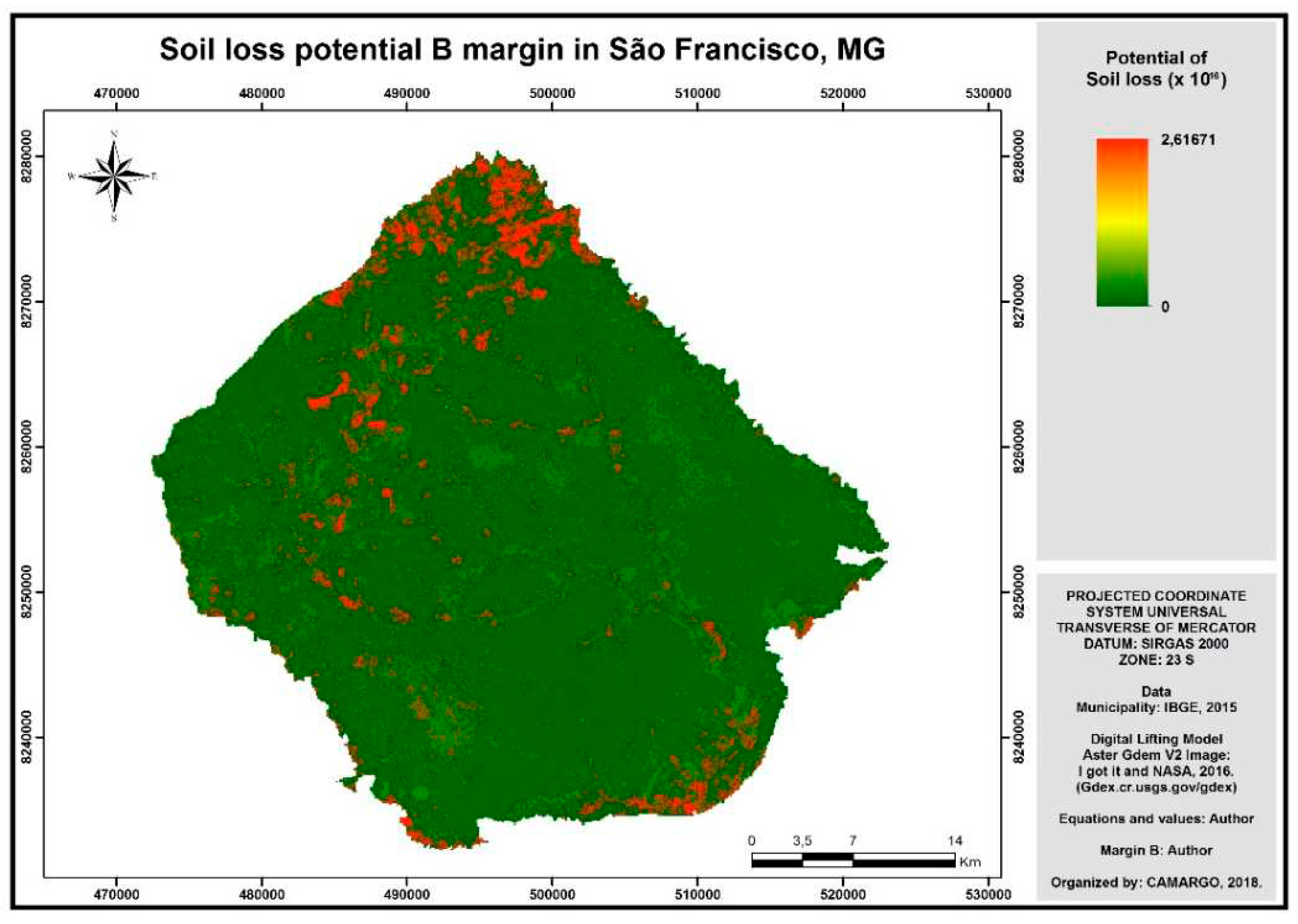
Figure 10.
Qualitative potential of soil loss in margin B in the municipality of San Francisco according to the new methodology used here.
Figure 10.
Qualitative potential of soil loss in margin B in the municipality of San Francisco according to the new methodology used here.
Comparing the final map obtained here with the representative map of the same site using the traditional methodology (Figure 11), it is possible to observe a great qualitative similarity between both, and therefore, as in the case of R calculation, indicated the use of statistical tools to verify whether the present similarity is in fact mathematically thalking.
Statistical tests to verify correlation between both methodologies of calculation of laminar soil loss
As with erosivity, the results obtained in both forms were compared with the use of Excel basic statistical programs, in order to obtain the degree of similarity between both forms (using the Pearson correlation test), the classic and the developed here, generating in this way the Figure 12.
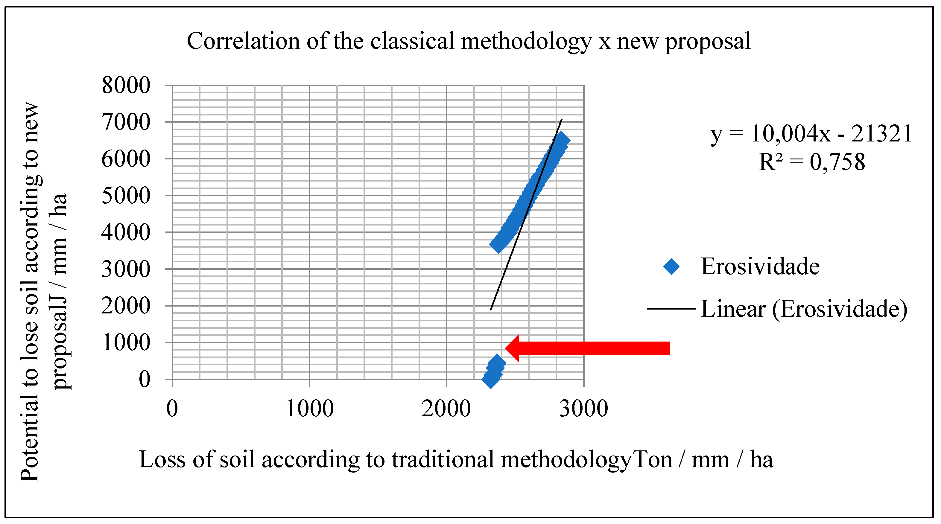
Figure 12.
Correlation test between both qualitative methodologies of laminar soil loss.
According to Figure 12, a degree of correlation higher than 75% (0.758) can be noticed between both forms. According to Cohen (1988) [3] and corroborated by Dancey and Reidy (2006) [4], this result can be characterized as having a high statistical affinity, which proves that both methodologies present similar results, mathematically recommending the new proposal developed here for the qualitative verification of the laminar soil loss.
3.5. Understanding the results obtained 2
The new form for qualitative calculation of A was statistically correct when compared to the conventional model, which shows great success in the methodology proposed here. However, as in the case of erosivity, there is no guarantee that this is a universal truth, only for the case of margin B of the municipality of São Francisco, which in itself already shows a great novelty in the study of soils taking into account view that this form of qualitative measurement is unprecedented.
Again, more studies are indicated in different areas to make sure that this new tool serves any type of site, but it is undeniable to think that, just as in the case of R calculation, such statistical similarity is very surprising.
Silva and Machado (2014) [17] used the GIS for erosive verification in Nova Lima (MG) and had satisfactory results in their research. The use of indirect forms and consequent calculation of laminar soil loss is not something new. Likewise, Lopes et. al. (2011) [10] also made use of geoprocessing to identify soil loss in the semi-arid region of Ceará, showing that the use of GIS in Geosciences becomes more and more usual. Mendonça et. al. (2014) [12] were other authors who worked with the use of EUPS for indirect estimation of soil loss in the municipality of Iconha (ES), obtaining also good results.
However none of these works or others in the literature dialogue with the method proposed here. The most similar is that of Lima et. al. (2007) [9], who as well as this study sought to develop new indirect techniques in pedological calculations in the Alto Jardim (DF) basin. The difference, in the case of the work of these authors with what is developed in this chapter is that Lima et. al. (2007) [9] worked with Factor K (erodibility) while studying R and EUPS.
It is also worth mentioning a curious difference when observing the correlation test (red arrow present in Figure 12) between both methodologies. A small part of the sampling points is shown outside the line corresponding to the similarity. These points correspond exactly to the North end of margin B, where there is a greater indication of laminar loss in Figure 11 (new form) than in Figure 10 (traditional).
The impacted Cerrado is the type of land use and occupation predominant in this range of the map (Figure 13). This helps to understand why this potential increase of laminar loss is present, because where the soil is more exposed, obviously more susceptible to erosion, it becomes.
Surprisingly, even the traditional method has not pointed out this important detail with so much emphasis on its final map, which further corroborates the importance of this new methodology proposed when compared to the classic model.
Thus, at least in the case of the study area that competes with this article, it can be concluded that the proposals presented here, both for the calculation of erosivity and the laminar loss of soil, both in a qualitative way, present results statistically similar to the methods traditional commonly used.
5. Conclusions
The paper in question was proposed to generate new forms of qualitative calculation of erosivity and laminar soil loss with the use of physical variables and GIS. Both proposals were carried out and proved to be successful when compared statistically with the traditional calculation methods, especially the EUPS.
Obviously, it is too early to say if this new indirect form used here constitutes a new universal proposal for calculating R and A, but for the study area of this paper, the proposal developed here can be used quietly, as it shows statistically similar results, from the qualitative point, to the traditional model.
When analyzing soil loss, especially laminar erosion, quantitative calculations do not serve in practice as environmental management tools, since the most important is to know where the soil presents loss potential to undergo some kind of corrective intervention. In this way, the results obtained here are extremely satisfactory considering the proposed method, which is only qualitative.
New studies are advised in different regions in order to verify if the new tool developed in this research can be used in any area beyond the research region.
Acknowledgments
The authors are grateful to the Department of Geology of the Federal University of Ouro Preto (UFOP) for the approval of the research project under the Postgraduate Program in Crustal Evolution and Natural Resources (PHD), as well as the Coordination of Improvement of Personnel (CAPES) for students' research grants.
References
- Bertoni, J.; Lombardi Neto, F. Conservação do solo. São Paulo. Editora Ícone 1990, 355p. [Google Scholar]
- Borges, K.M.R. Avaliação da susceptibilidade erosiva da Bacia do Rio Carinhanha (MG/BA) por meio da EUPS - Equação Universal de Perda de Solos. MS Dissertation. Departamento de Geografia, Universidade de Brasília, Brasília 2009, 68p. [Google Scholar]
- Cohen, J. Statistical power analysis for the behavioral sciences. Hillsdale, NJ, Erlbaum 1988, 487 p. [Google Scholar]
- Dancey, C.; Reidy, J. Estatística Sem Matemática para Psicologia: Usando SPSS para Windows. Porto Alegre, Artmed 2006, 608p. [Google Scholar]
- Foster, G.R.; Young, R.A.; Römkens MJ, M.; Onstad, C.A. Processes of soil erosion by water. In: Follet R.F., Stewart B.A. (eds.) Soil erosion and crop productivity. Madison, Soil Science Society of America 1985, 137–158. [Google Scholar]
- Fujihara, A.K. Predição de erosão e capacidade de uso do solo numa microbacia do Oeste Paulista com suporte em geoprocessamento. MS Dissertation, Escola Superior de Agricultura Luiz de Queiroz (ESALQ), Universidade de São Paulo, Piracicaba 2002, 118 p. [Google Scholar]
- Garson, G.D. Statnotes: Topics in Multivariate Analysis. 2009. Disponível em: http://faculty.chass.ncsu.edu/garson/PA765/statnote.htm (Acesso em Março de 2017).. [Google Scholar]
- Jacomine, P.K.T.; Cavalcanti, A.C.; Formiga, R.A.; Silva, F.B.R.; Burgos, N.; Medeiros, L.A.R.; Lopes, O.P.; Meio Filho, H.F.R.; Pessoa, S.G.P.; Lima, P.C. Levantamento exploratório - reconhecimento de solos do Norte de Minas Gerais; área de atuação da SUDENE. Recife, EMBRAPA/SN LCS—SUDENE/DRN, Boletim Técnico 60, 1979, 408p. [Google Scholar]
- Lima, J.E.F.W.; Silva, E.M.; Eid, N.J.; Martins, E.S. Desenvolvimento e verificação de métodos indiretos para a estimativa da erodibilidade dos solos da bacia experimental do Alto Rio Jardim – DF. Revista Brasileira de Geomorfologia 2007, 8, 23–36. [Google Scholar] [CrossRef]
- Lopes, F.B.; Andrade, E.M.; Teixeira, A.S.; Caitano, R.F.; Chaves, L.C.G. Uso de geoprocessamento na estimativa da perda de solo em microbacia hidrográfica do semiárido brasileiro. Revista Agro@mbiente On-line 2011, 5, 88–96. [Google Scholar] [CrossRef]
- Mello, G.; Bueno CR, P.; Pereira, G.T. Variabilidade espacial de perdas de solo, do potencial natural e risco de erosão em áreas intensamente cultivadas. Revista Brasileira de Engenharia Agrícola e Ambiental 2005, 10, 315–322. [Google Scholar] [CrossRef]
- Mendonça, R.F.P.; Paterlini, E.M.; Oliveira, F.S.; Barbosa, R.P.; Santos, A.R. Estimativa de perda de solo por erosão laminar para o município de Iconha, estado do Espírito Santo. Enciclopédia Biosfera, Goiânia 2014, 10, 1027–1038. [Google Scholar]
- Moore, D.S. The Basic Practice of Statistics. New York, Freeman 2007, 654p. [Google Scholar] [CrossRef]
- Odum, H.T. Environmental Accouting. Emergy and Environmental Decision Making. New York, John Wiley & Sons, Inc. 1996, 359p. [Google Scholar]
- Teixeira., M.B.; Camargo, P.L.T.; Martins Júnior, P. Avaliação da perda universal de solos para o município de São Francisco - Minas Gerais. Revista Geografia Acadêmica 2017, 11, 67–78. [Google Scholar]
- Silva, A.M.; Schulz, H.E.; Camargo, P.B. Erosão e hidrossedimentologia em bacia hidrográficas. RIMA Editora, São Carlos 2004, 138p. [Google Scholar]
- Silva, V.C.B.; Machado, P.S. SIG na análise ambiental: susceptibilidade erosiva da bacia hidrográfica do Córrego Mutuca, Nova Lima – Minas Gerais. Revista de Geografia (UFPE) 2014, 31, 66–87. [Google Scholar]
- Stein, D.P.; Donzelli, P.; Gimenez, A.F.; Ponçano, W.L.; Lombardi Neto, F. Potencial de erosão laminar natural e antrópica na bacia do Peixe Paranapanema. In: 4º Simpósio Nacional de Controle de Erosão. Marília 1987, 105–135. [Google Scholar]
- Wischmeier, W.H.; Smith, D.D. Predicting rainfall erosion losses – a guide for conservation planning. U.S. Department of Agriculture Agriculture Handbook 1978, 537, 58 p. [Google Scholar]
| 1 | It should be noted that only this software allows the programmed use of the mapping described here. Therefore, similar and free mapping platforms are not possible to realize the methodologies described here by limitations present in their use tools. |
Figure 1.
Study area.
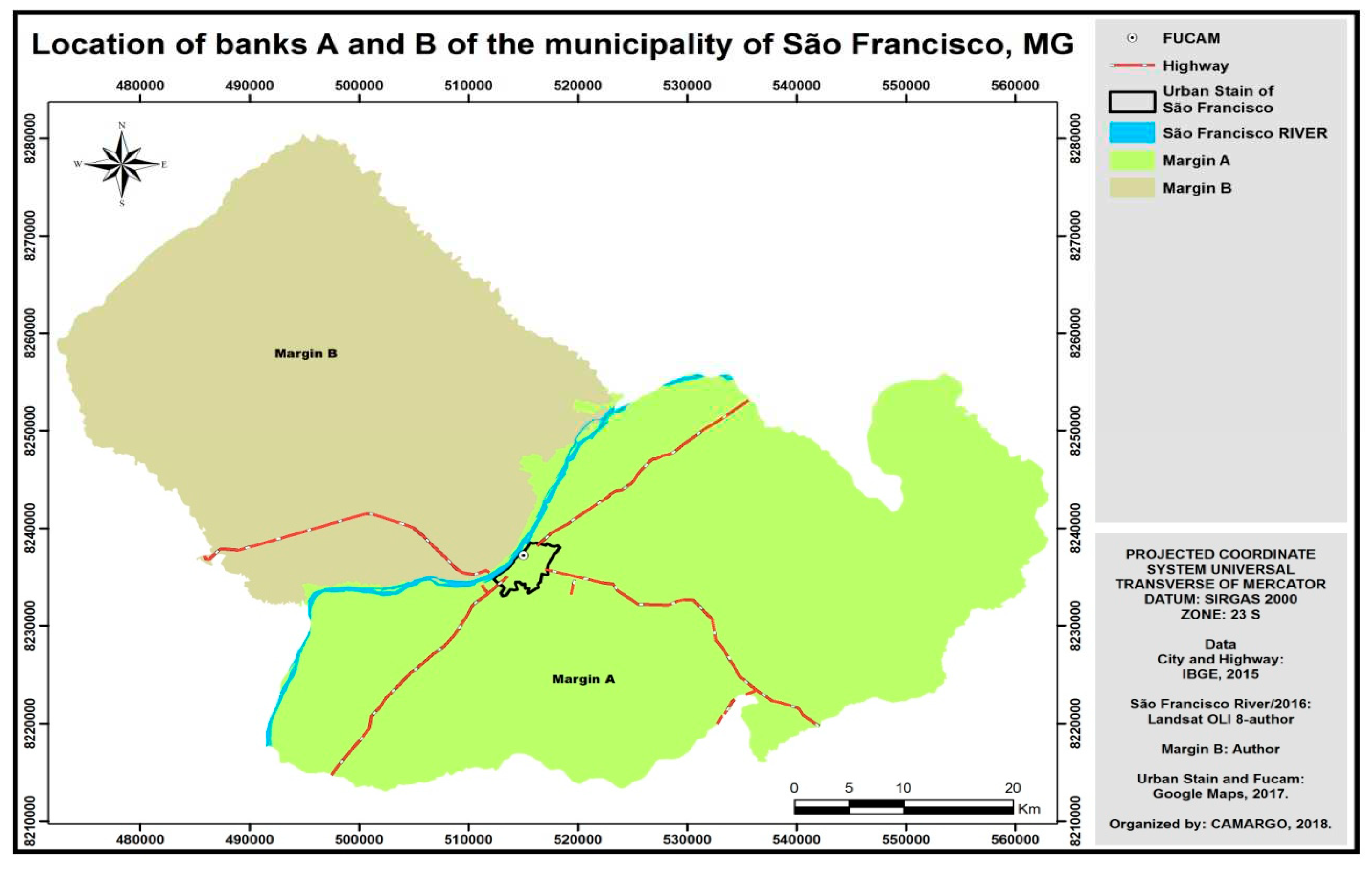
Figure 2.
Map of Hypsometry of municipality of San Francisco.
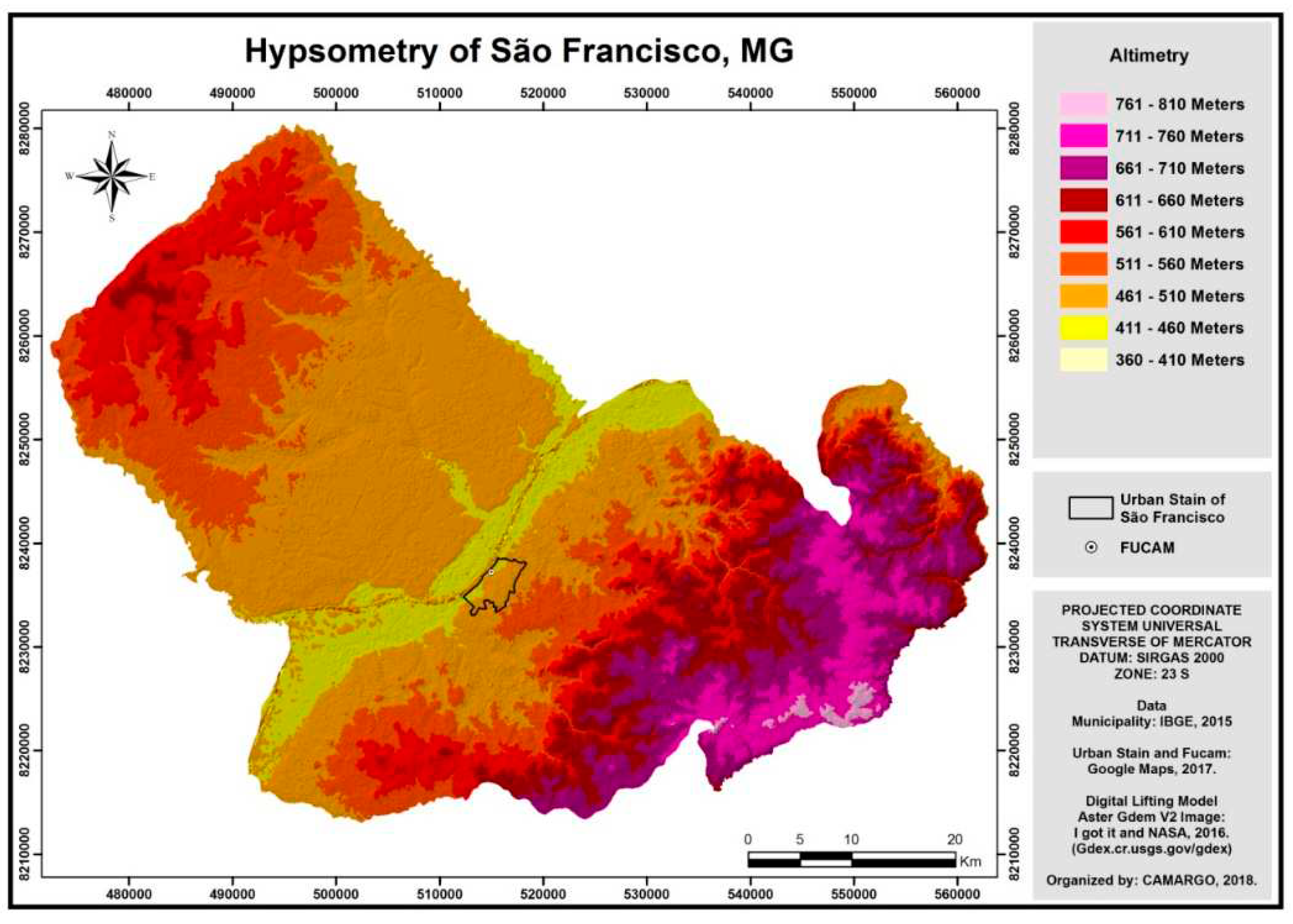
Figure 3.
Map of the physical energy of rain in the municipality of San Francisco.
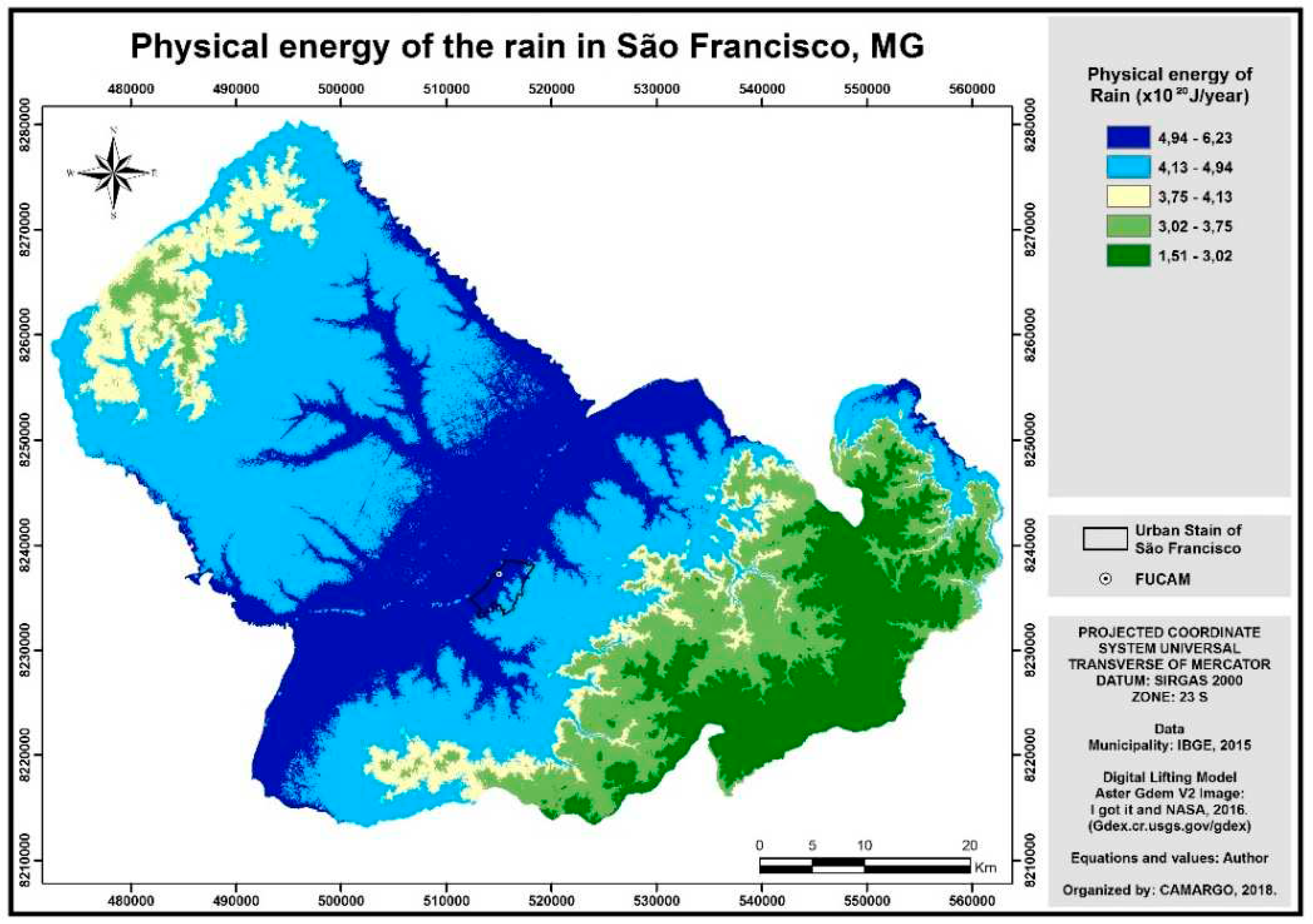
Figure 4.
Rainfall map in the municipality of San Francisco.
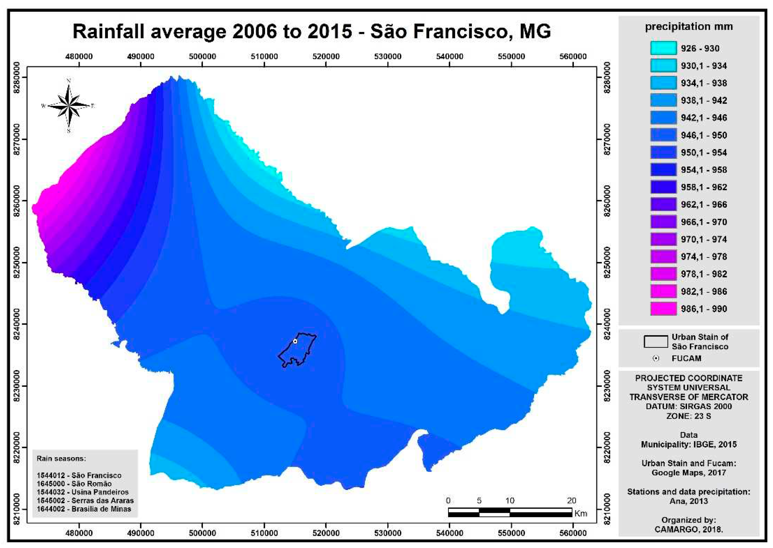
Figure 5.
Map of erosivity (R) in the municipality of San Francisco.
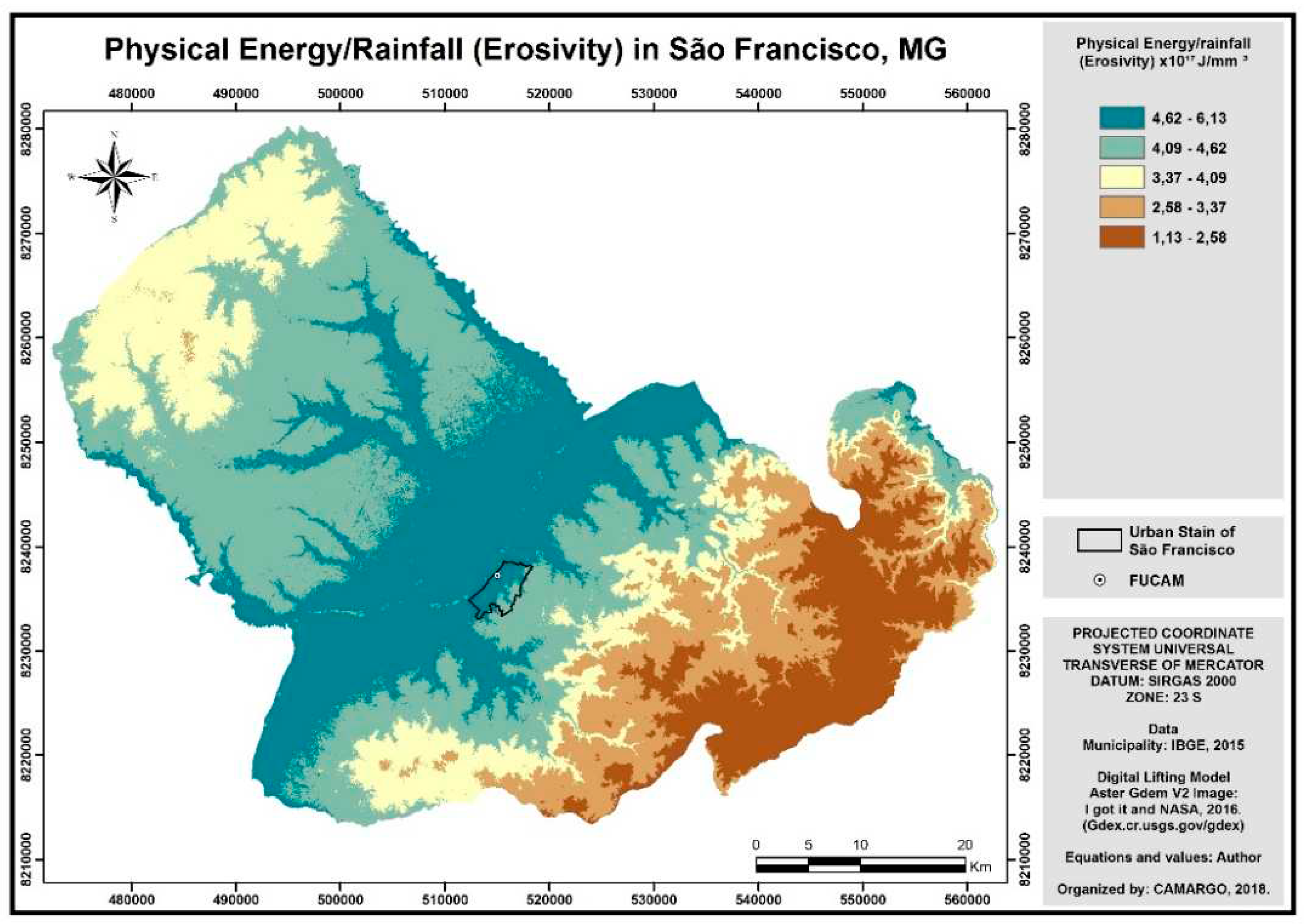
Figure 6.
Map of erosivity (R) in margin B (qualitative) in the municipality of San Francisco according to the conventional method (Teixeira et. al. (2017b, p.73)) [15].
Figure 6.
Map of erosivity (R) in margin B (qualitative) in the municipality of San Francisco according to the conventional method (Teixeira et. al. (2017b, p.73)) [15].
Figure 7.
Correlation chart between both methodologies of qualitative calculation of erosivity.

Figure 8.
Potential soil loss for erosivity in the municipality of San Francisco.
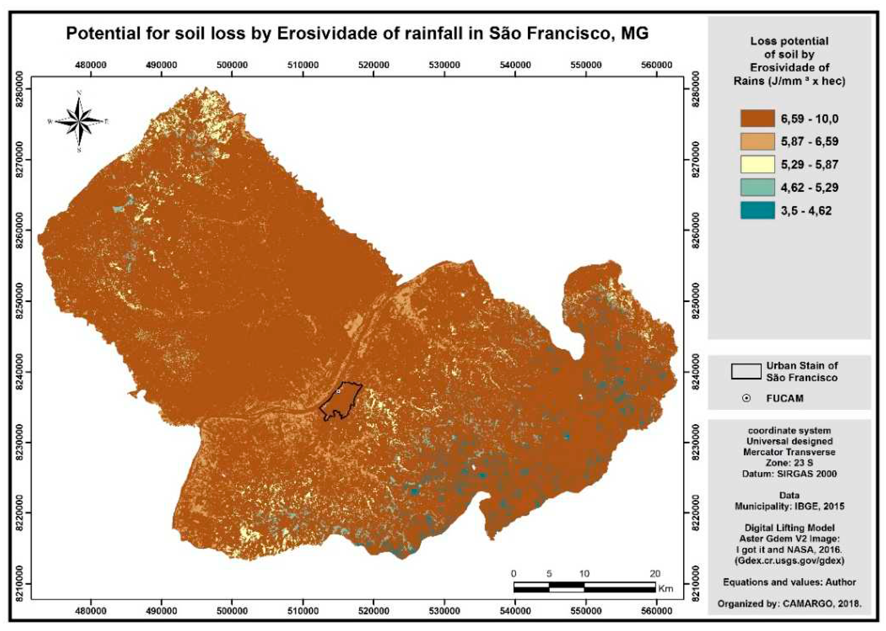
Figure 9.
Factor K present in margin B in the municipality of San Francisco (Source: Teixeira et. al. (2017b, p. 73)) [15].
Figure 9.
Factor K present in margin B in the municipality of San Francisco (Source: Teixeira et. al. (2017b, p. 73)) [15].
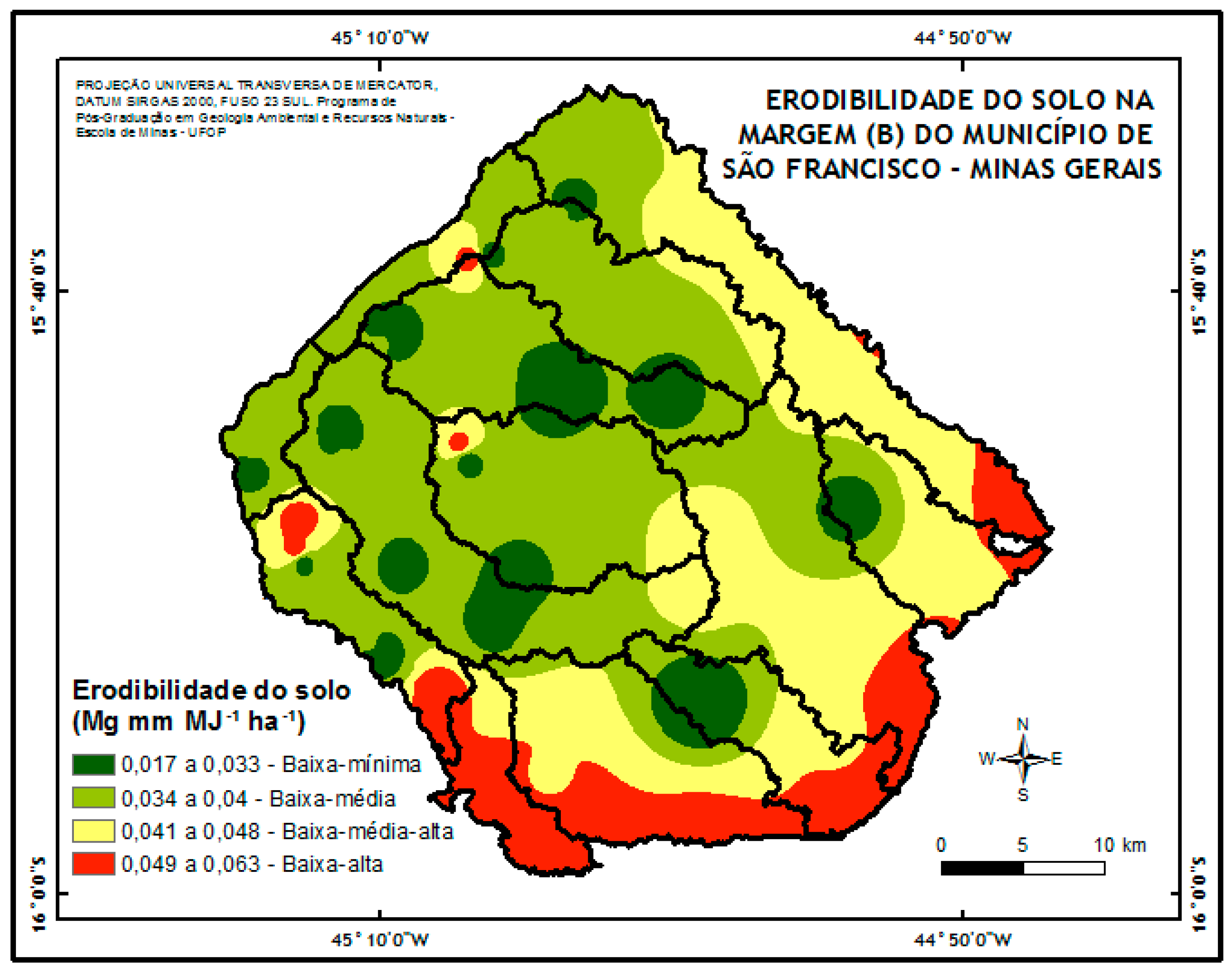
Figure 11.
Soil loss potential in the B margin in the municipality of San Francisco according to the classical methodology (Source: Teixeira et. al. (2017b, p.74)) [15].
Figure 11.
Soil loss potential in the B margin in the municipality of San Francisco according to the classical methodology (Source: Teixeira et. al. (2017b, p.74)) [15].
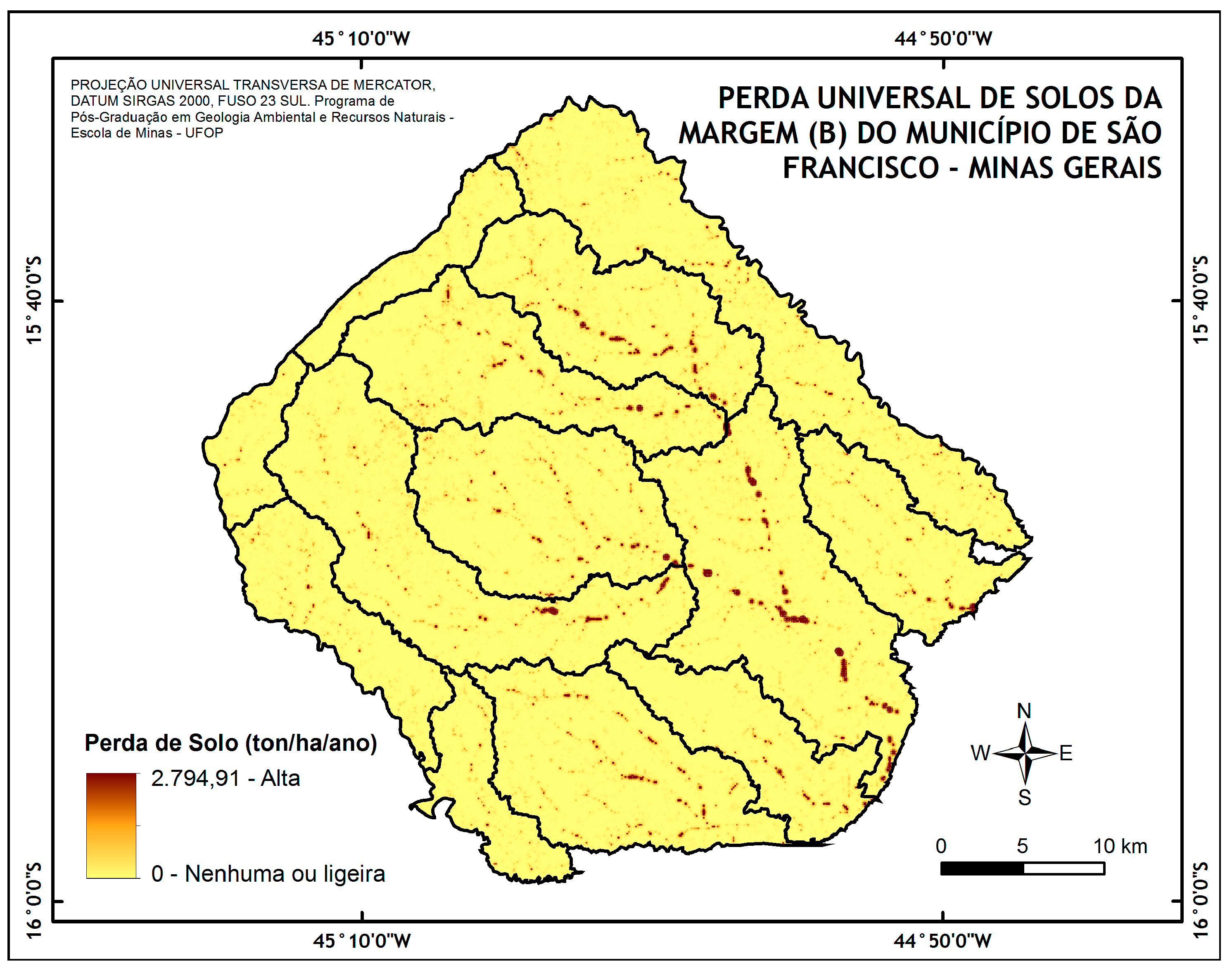
Figure 13.
Presence of Cerrado Impact in margin B in the municipality of San Francisco (Source: Teixeira et. al. (2017b)) [15].
Figure 13.
Presence of Cerrado Impact in margin B in the municipality of San Francisco (Source: Teixeira et. al. (2017b)) [15].
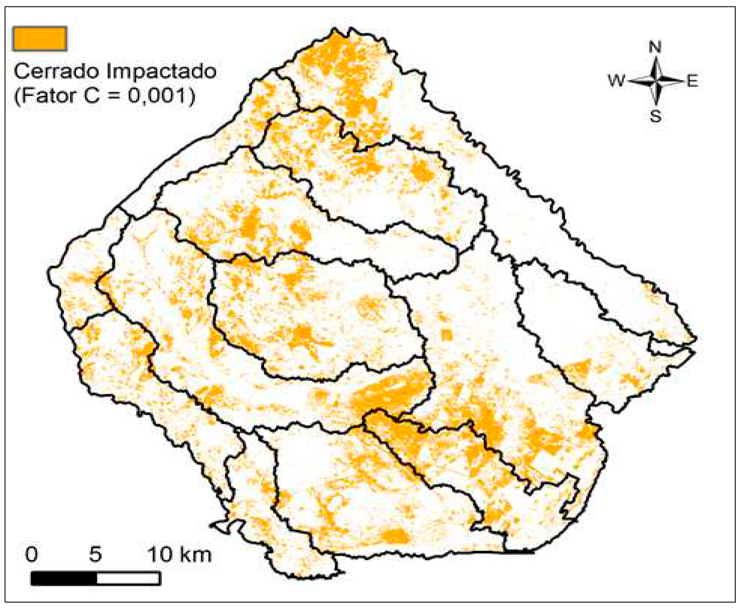

Table 1.
Soil Use x Factor C.
| Soil Use | Factor C |
|---|---|
| Water | 0 |
| Low Native Vegetation (Cerrado) | 0,001 |
| Dense Native Vegetation (Others) | 0,002 |
| Farming Activities | 0,75 |
| Soil Exposed | 1 |
| Urban Area | 0,03 |
Disclaimer/Publisher’s Note: The statements, opinions and data contained in all publications are solely those of the individual author(s) and contributor(s) and not of MDPI and/or the editor(s). MDPI and/or the editor(s) disclaim responsibility for any injury to people or property resulting from any ideas, methods, instructions or products referred to in the content. |
© 2023 by the authors. Licensee MDPI, Basel, Switzerland. This article is an open access article distributed under the terms and conditions of the Creative Commons Attribution (CC BY) license (http://creativecommons.org/licenses/by/4.0/).
Copyright: This open access article is published under a Creative Commons CC BY 4.0 license, which permit the free download, distribution, and reuse, provided that the author and preprint are cited in any reuse.


