Preprint
Article

Uncovering Top-Tier Machine Learning Classifier for Drinking Water Quality Detection

Altmetrics

Downloads

203

Views

86

Comments

0

This version is not peer-reviewed

Submitted:

22 August 2023

Posted:

24 August 2023

You are already at the latest version

Alerts
Abstract
Water quality assessments are crucial for human health and environmental safeguards. The utilization of a subset of artificial intelligence such as Machine Learning (ML) presents significant impacts to enhance the prediction and classification of water quality. In this research, a set of diverse ML algorithms was evaluated to handle a comprehensive dataset of water quality measurements over an extended period. The aim was to develop a robust approach for accurately forecasting water quality. This approach employed machine learning classifiers such as Logistic Regression (LR), Support Vector Machine (SVM), Stochastic Gradient Descent (SGD), K-Nearest Neighbors (KNN), Gaussian Process Classification (GPC), Gaussian Naive Bayes (GNB), Random Forest (RF), Decision Tree (DT), XGBoost, and Multilayer Perceptron (MLP). The water quality parameters assessed for pH, hardness, solids, chloramines, sulfate, conductivity, organic carbon, trihalomethanes and turbidity. The XGBoost model exhibited the highest accuracy of 89.47% among the classifiers and Stacked Ensemble Classifiers (SEC) improved the prediction further to 92.98%. The findings suggest that XGBoost and the SEC hold promise as reliable approaches for water quality assessments in contrast of artificial intelligence.
Keywords: 
Subject: Engineering  -   Civil Engineering

1. Introduction

Drinking water quality is one of the greatest factors affecting human health [1,2,3,4]. Drinking water quality is a paramount concern worldwide, as it directly affects human health and well-being. Access to clean and safe drinking water is vital for preventing waterborne diseases and ensuring public health [5,6,7,8]. The assessment and management of drinking water quality have emerged as crucial fields, addressing the need for continuous monitoring and maintenance of water supplies. Numerous research articles highlight the risks associated with contaminated drinking water, including the transmission of waterborne diseases, adverse health effects, and potential long-term consequences on the overall well-being of individuals and communities [9,10,11]. Consequently, the importance of maintaining high standards of drinking water quality is widely recognized in the scientific community as a fundamental necessity for safeguarding public health and promoting sustainable development. However, drinking water quality in many countries, especially in developing countries, is not desirable and poor drinking water quality has induced many waterborne diseases [12,13].
Having access to safe drinking water is a basic human right to all people, regardless of nationality, religion, color, wealth or creed. Contaminated drinking water and poor sanitation are linked to transmission of waterborne diseases and significantly affecting the health of more than 2 billion people over the world [14,15,16]. In recent years, many developing countries have set reduction of waterborne diseases and development of safe water resources as their major public health goal, and the situation has slightly improved [17]. The rigorous and systematic investigation of drinking water quality determination is essential for the protection of public health and the development of more accurate and efficient testing methods. The effective and efficient pursuit of knowledge on drinking water quality determination is critical to ensuring the safety and sustainability of our water resources [18,19,20]. Commonly, assessing WQ entails collecting water samples from various sites at different time intervals and evaluating them in laboratories. However, manual sampling and laboratory analysis of WQ for any given water body or process can be inefficient, expensive and time consuming. As a result, intelligent systems are increasingly used to monitor WQ, especially when real-time data are needed [21,22,23,24].
With the rapid increase in the volume of data on the aquatic environment, machine learning has become an important tool for data analysis, classification, and prediction [25,26,27,28,29]. Unlike traditional models used in water-related research, data-driven models based on machine learning can efficiently solve more complex nonlinear problems [30,31,32,33,34]. Machine learning models have shown great potential in the estimation and prediction of water quality parameters, offering improved accuracy and efficiency compared to traditional methods. These models have the capability to analyze large volumes of data, identify complex patterns, and provide valuable insights for water quality assessment and management, making them valuable tools in the field of water resources and environmental engineering [35,36,37,38]. Despite the significant advancements in machine learning, its adoption in predicting and automating drinking water processes has been relatively limited [39,40,41,42]. The complexity and variability of water quality parameters, coupled with the need for robust and interpretable models, present challenges in effectively implementing machine learning approaches in this domain. However, with further research and development, there is immense potential for machine learning to revolutionize the prediction and automation of drinking water systems, enhancing operational efficiency, water quality monitoring, and decision-making processes [43,44,45,46].
Water utilities are required to provide consumers with reliable access to clean and affordable drinking water. To achieve this, water must be sourced from reliable and sufficient freshwater sources and treated to meet regulatory and industry standards [47,48,49,50]. Factors such as consumer acceptance, effective treatment procedures, and efficient utility management are crucial in ensuring the quality of drinking water. High-quality water should be free from harmful organisms and biological forms, visually appealing, clear, colorless, odorless, and tasteless. It should also be free from chemicals that may pose health risks or cause aesthetic issues and should not cause corrosion or deposits in water infrastructure [51,52,53].
In previous studies, an Artificial Neural Network and time series analysis were utilized to develop a water quality prediction model. Model performance was evaluated using metrics such as Mean Squared Error (MSE), Root Mean Squared Error (RMSE), and Regression Analysis. Previous researchers employed 12 machine learning models to estimate water quality, and the models were evaluated using R2 and RMSE statistics. They utilized supervised machine learning algorithms to estimate the Water Quality Index. They applied 8 artificial intelligence algorithms to predict the Water Quality Index, and model evaluation involved statistical metrics such as correlation coefficient (R), mean absolute error (MAE), RMSE, relative absolute error (RAE), and root relative square error (RRSE) [54,55,56].
The objectives of this study are as follows: (i) Initial evaluation of the available data was conducted to filter, normalize, and implement classification algorithms for predicting drinking water quality and identifying the most suitable combination of water quality parameters. This can potentially eliminate the need for costly and time-consuming lab analyses with specific sensors in future similar investigations. (ii) Various classification techniques were selected as examples and proposed for the comprehensive analysis of numerical water quality. (iii) Multiple ML classifiers, including Logistic Regression (LR), Support Vector Machine (SVM), Stochastic Gradient Descent (SGD), K-Nearest Neighbors (KNN), Gaussian Naive Bayes (GNB), Random Forest (RF), Decision Tree (DT), XGBoost, and Multilayer Perceptron (MLP), were applied to the dataset to detect water quality [57,58,59,60,61].

2. Methods

The data for this method was sourced from Kaggle's Water Quality Dataset, which included various parameters such as hardness, sulfate, solid, trihalomethanes, pH, turbidity, solids, organic carbon, and electrical conductivity. We divided the information into features (Table 1) and the target variables because our objective was to create a model that can determine the water quality as a function of other input features.

2.1. Multivariate Exploratory Data Analysis (MEDA)

To understand the properties and characteristics of the multivariate dataset, a thorough Exploratory Data Analysis (MEDA) was carried out. The crucial stage in performing MEDA on data is to do so in order to get the ML model to operate well. All the drinking water quality variables' internal distribution was examined using a variety of visual techniques and numerical indexes. MEDA is the process of conducting an initial inquiry into the drinking water quality variables to identify any hidden patterns in the variables' distribution [62,63]. MEDA is further broken down into a variety of activities. They are known as the normality check, outliers/extreme values identification, and descriptive statistics. With the help of the number of data points, mean, standard deviation, percentiles, interquartile range, and range of the variables, descriptive statistics offer a fantastic method for illustrating the distribution of their values. displays complete multivariate descriptive statistics. Histograms with density plots are used as a visual representation to show the normality of the variables, and Pearson's coefficient of skewness (PCS) is used as a numerical measure of skewness. By substituting the Nearest Neighbors (NN) of the datapoints for missing values, numerical imputation is used to make the dataset consistent.
Table 2. Descriptive Statistics of the water quality variables.
Ph Hardness Solids Chloramines Sulfate Conductivity Organic_carbon Trihalomethanes Turbidity Potability
count 2785.00 3276.00 3276.00 3276.00 2495.00 3276.00 3276.00 3114.00 3276.00 3276.00
Mean 7.08 196.37 22014.09 7.12 333.78 426.21 14.28 66.40 3.97 0.39
Std 1.59 32.88 8768.57 1.58 41.42 80.82 3.31 16.18 0.78 0.49
Min 0.00 47.43 320.94 0.35 129.00 181.48 2.20 0.74 1.45 0.00
25% 6.09 176.85 15666.69 6.13 307.70 365.73 12.07 55.84 3.44 0.00
50% 7.04 196.97 20927.83 7.13 333.07 421.88 14.22 66.62 3.96 0.00
75% 8.06 216.67 27332.76 8.11 359.95 481.79 16.56 77.34 4.50 1.00
Max 14.00 323.12 61227.20 13.13 481.03 753.34 28.30 124.00 6.74 1.00
Figure 1's graphic representation of the distribution of the variables demonstrates the significant level of overall non-normality. When compared all the variables exhibited more non-normality. The values of -0.8 (pH), -0.04 (Hardness), 0.62 (Solids), -0.01 (Chloramines), 0.02 (Sulfate), 0.27 (Conductivity), 0.03 (Organic Carbon), 0.15 (Trihalomethanes), -0.01 (Turbidity) and 0.45 (Potability) are Pearson's Skewness Coefficient (PSC), a numerical indicator of non-normalcy/skewness, are likewise greater than the PCS values of other drinking water quality variables, indicating considerably less normality.
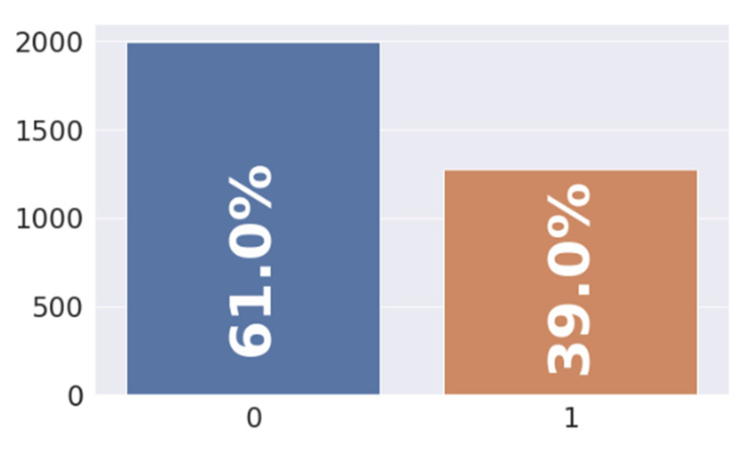
The dataset used in this study consists of various water quality variables, including pH, Hardness, Solids, Chloramines, Sulfate, Conductivity, Organic Carbon, Trihalomethanes, and Turbidity, with the target variable being Water Potability. Descriptive statistics were computed for each variable, providing insights into the distribution and variability of the data. From the statistics, it can be observed that the mean pH is 7.08, with a standard deviation of 1.59, indicating a moderately acidic to neutral range. Similarly, other variables exhibit varying means and standard deviations. The Potability variable shows that approximately 61% of the samples are classified as potable water. These descriptive statistics provide a preliminary understanding of the dataset and lay the foundation for further exploratory data analysis and modeling techniques to investigate the relationships between water quality parameters and potability status. This study aims to utilize machine learning algorithms to develop a predictive model for water potability, contributing to the field of water resource management and public health.
Figure 2. Distribution of the target variable, y in percentage for potability feature.
Preprints 83007 g002
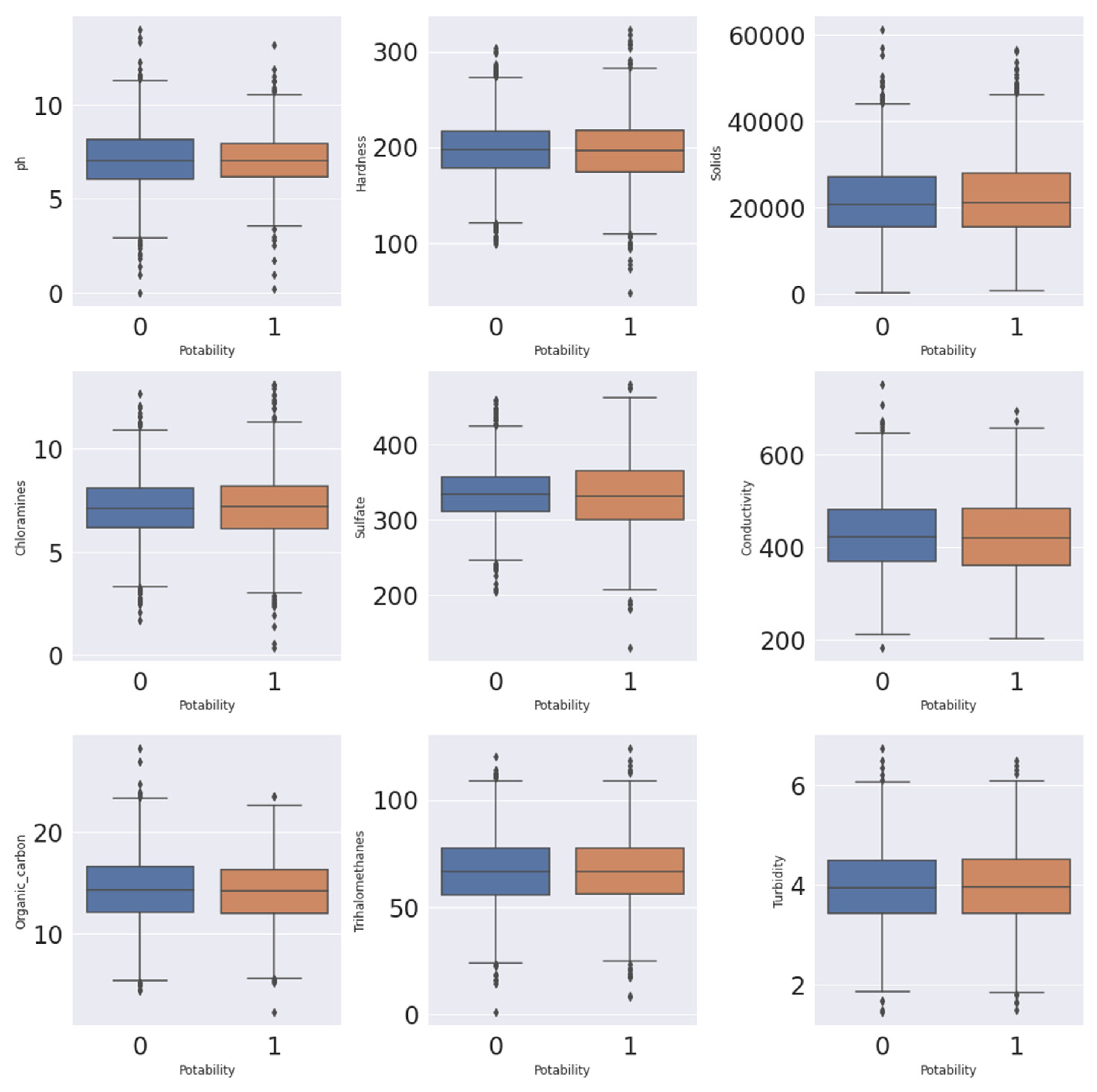
The joint distribution between each input feature (pH, Hardness, Solids, Chloramines, Sulfate, Conductivity, Organic Carbon, Trihalomethanes, Turbidity) and the target variable (Water Potability) provides valuable insights into the relationship between water quality parameters and potability status. By examining the joint distribution, we can assess the conditional probabilities and dependencies between these variables.
This analysis helps in understanding how changes in the input features impact the potability of water. Understanding the joint distribution is crucial for identifying significant patterns and correlations that may exist within the data. It enables us to uncover potential relationships between specific water quality characteristics and the likelihood of water being potable or non-potable. By exploring the joint distribution, we can gain insights into the factors that contribute to water potability and prioritize them accordingly in further analysis and modeling.
Figure 3. Joint distribution of the input (x) and target variables (y) using the boxplots.
Preprints 83007 g003

2.2. Feature Engineering

After an initial analysis of the dataset using MEDA, the next step involves conducting feature engineering (FE). The success of the ML approach greatly depends on effective FE, as it ensures accurate and satisfactory performance. To achieve optimal results using iterative gradient descent, a comprehensive examination of the dataset is crucial. Hence, a meticulous feature engineering process is employed to transform variables into forms that best suit the ML algorithms. This study incorporates techniques such as imputation, data transformation, data normalization, and the division of the dataset into training, testing, and validation sets as part of the FE process. Imputation is employed to address null values and enhance overall dataset consistency. Sensor errors resulted in certain series containing missing values or observations. In this study, the missing values were imputed with values from the nearest neighbors, as excluding these observations would reduce the dataset size and hinder implementation. After successful imputation using the median values, the distribution of the variable series is assessed visually and quantitatively to verify normality. One measure of normality is the PCS. The discharge and water level variables exhibit significantly non-normal distributions with a pronounced left skew, which poses challenges for achieving satisfactory optimization in neural network regression algorithms.
Because the variable under study in this study is a continuous independent variable, normalizing the variable is crucial for training and assessing the neural network algorithm. The normalizing technique is required for the optimization. The gradient descent method is used by the ML classification model, and the feature value affects the method's step size. Smooth progress towards minima in gradient descent requires updating the steps for all feature values at the same rate. In the gradient descent process, a normalized variable is necessary to get to the lowest point. To create the training dataset for the ML model, the values are all normalized. The normalization formula for variable series is presented in Equation (1).
X n o r m = X X m i n X m a x X m i n  
In the formula, X represents the relevant variable, and the subscripts norm, max, and min denote the maximum and minimum values of the normalized variable. The series range is divided by the difference between the variable of interest and the minimum value of the entire series, resulting in normalized data that is utilized during the training and testing stages of the ML process. The set of normalized variables is divided into two parts: a training set, utilized for model training, and a testing set, employed to assess and evaluate the model.

2.3. Machine Learning Classifiers

We established the necessary methods and tools to enable a model to make accurate forecasts. These tools and methodologies greatly enhance the confidence in the forecasts by allowing for precise evaluation of each model's performance. To assess the quality of a given model, its performance on both the training and testing sets must be quantified. Typically, performance metrics such as error computation, goodness of fit, or other relevant measurements are utilized. In this project, we will partition the drinking water quality dataset into training and testing subsets, ensuring that the data is randomly shuffled to eliminate any bias in the dataset ordering. Once trained, a model is evaluated to determine its ability to learn from the training data. There are three possible scenarios: underfitting, where the model poorly learns from the data and cannot predict even the training set results due to high bias; overfitting, where the model memorizes the training data and fails to generalize to new data due to high variance; and optimal learning, where the model accurately predicts results on new data, striking the right balance between bias and variance. In this study, we developed a robust approach for accurately forecasting water quality, employing various machine learning classifiers including LR, Support Vector Machine (SVM), SGD, KNN, Gaussian Process Classification (GPC), GNB, RF, DT, XGBoost, and MLP.

2.4. Hyperparameters Optimization

In this study, hyperparameter tuning was performed for the various machine learning classification models. For each model, a systematic approach was employed to identify the optimal combination of hyperparameters that maximized performance on the drinking water quality determination task. This involved conducting a grid search over a predefined range of hyperparameter values, considering parameters such as regularization strength, learning rate, number of neighbors, number of estimators, maximum tree depth, and hidden layer sizes. The performance of each model was evaluated using appropriate evaluation metrics such as accuracy, precision, recall, and F1-score. The hyperparameters yielding the best performance for each model were selected for the final analysis, ensuring robust and optimized classification performance for drinking water quality determination.

2.5. Error Analysis

A wide range of evaluation metrics are available in the literature to assess the accuracy of supervised classification methods. These metrics quantify the discrepancy between the anticipated values and the measured values of data points, as determined through various techniques, capturing the error in the predictions. In this study, different error matrices were utilized to assess the variability of the models. One commonly used measure is the confusion matrix, which is applicable to both binary and multiclass classification problems. The confusion matrix provides counts for predicted and actual values, with "TN" representing True Negative (accurately classified negative examples), "TP" representing True Positive (accurately classified positive examples), "FP" indicating False Positive (actual negative examples classified as positive), and "FN" representing False Negative (actual positive examples classified as negative). The F-score, or F-measure, is a statistical measure used to assess the accuracy of a binary classification test. It combines precision and recall, where precision represents the ratio of true positive results to all positive results (including false positives), and recall represents the ratio of true positive results to all actual positive samples. Precision is also referred to as positive predictive value, while recall is known as sensitivity in diagnostic binary classification.

3. Results and Discussion

3.1. Predicted and Observed Data

The machine learning (ML) models are deployed to forecast the drinking water quality for testing after a successful training using the obtained drinking water quality data. The classification model’s performance is visually represented in Figure 5 by a scatterplot that compares predicted drinking water quality values to observed drinking water quality values.
The chosen hyperparameters are used to run the RF regressor (number of trees = 100, minimum number of samples needed to divide an internal node = 10, minimum number of samples needed to be at a leaf node = 1). Maximum tree depth is 50, number of features to be considered while determining the appropriate split is "sqrt," Whether bootstrap samples are used while creating trees is set to True, and the randomness of bootstrapping samples after optimization is set to 0. The chosen hyperparameters for MLP are the size of the hidden layers (100, 50), the activation function (ReLU, Sigmoid), the solver (Adam), the alpha (0.0001), and the learning rate (constant). The Rs values for the RF and MLP algorithms' training sets are 0.734 and 0.672, respectively. In the testing phase using an unknown dataset, both models perform worse and have lower R2 values (0.698 and 0.648).
In Figure 5, the fitted regression line's (black lines) statistical distance from the expected drinking water quality values is measured statistically by R2. where the values of observed and expected drinking water quality are the same.

3.2. Model Performance Evaluation

The Jaccard score, commonly used in machine learning classification tasks, measures the similarity between two sets by calculating the ratio of the size of their intersection to the size of their union. The Jaccard score is not often applied directly in regression tasks. Instead, it is more frequently used to examine how well classification algorithms function by comparing the accuracy of predicted classes to actual classes. Metrics like Mean Squared Error (MSE), Root Mean Squared Error (RMSE), and Mean Absolute Error (MAE), which measure the accuracy of projected continuous values against actual values, are more relevant for regression employment. Tabulated results of a comparison analysis of the model's performance using the XGB and KNN (Table 3). With a F1-score score of 0.93, the RF method surpasses other methods in forecasting channel drinking water quality, while its respective Jaccard are 0.89.
The Logistic Regression model achieved an accuracy of 60.57%. It demonstrated a precision of 48.00% and a recall of 11.85%. The F1-Score was 0.19, reflecting a balance between precision and recall. The K-Nearest Neighbors model achieved an accuracy of 59.41%. It exhibited a precision of 51.10% and a recall of 47.38%. The F1-Score was 0.49, indicating a harmonious trade-off between precision and recall. The Support Vector Machine model achieved an accuracy of 49.14%. It showed a precision of 40.85% and a recall of 54.68%. The F1-Score was 0.46, suggesting a balance between precision and recall. The Decision Tree model demonstrated exceptional performance with an accuracy of 98.83%. It exhibited a precision of 97.77% and a recall of 98.95%. The F1-Score of 0.98 indicated a robust balance between precision and recall. The Gaussian Naive Bayes model achieved an accuracy of 58.43%. It had a precision of 45.78% and a recall of 25.54%. The F1-Score was 0.33, suggesting a trade-off between precision and recall. The Gaussian Process Classifier achieved an accuracy of 71.33%. It demonstrated a precision of 66.67% and a recall of 48.98%. The F1-Score of 0.56 reflected a balance between precision and recall. In summary, the Decision Tree model stood out with exceptional accuracy, precision, recall, and F1-Score. The other models showed varying levels of performance, each with distinct strengths and limitations. The selection of a suitable model should consider the specific application requirements and trade-offs.
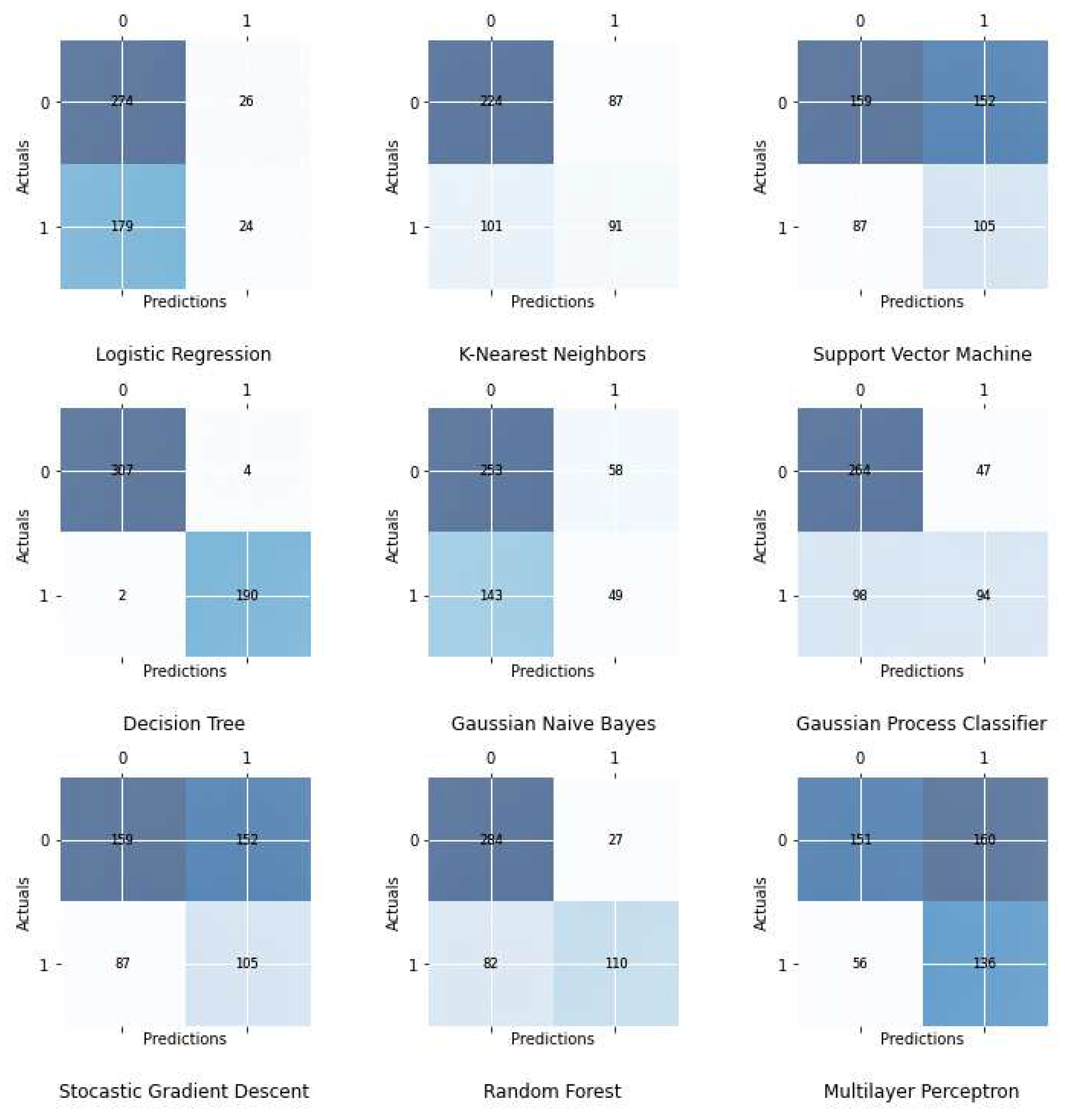
The confusion matrix analysis provides valuable insights into the classification performances of the different models. For instance, in the case of the Logistic Regression model, the confusion matrix indicates that it correctly predicted 274 instances of one class (True Negatives) and 24 instances of the other class (True Positives), but it misclassified 26 instances of the first class as the second class (False Positives) and 179 instances of the second class as the first class (False Negatives).
Similarly, the K-Nearest Neighbors model's confusion matrix shows that it accurately predicted 224 instances of one class and 91 instances of the other class, but it misclassified 87 instances of the first class and 101 instances of the second class.
The confusion matrix of the Support Vector Machine model demonstrates that it correctly classified 159 instances of one class and 105 instances of the other class, while misclassifying 152 instances of the first class and 87 instances of the second class. The Decision Tree model's confusion matrix highlights its remarkable performance, as it accurately predicted 307 instances of one class and 190 instances of the other class, with only 4 instances misclassified as the second class and 2 instances misclassified as the first class. The Gaussian Naive Bayes model's confusion matrix reveals that it correctly classified 253 instances of one class and 49 instances of the other class, but it misclassified 58 instances of the first class and 143 instances of the second class. Lastly, the Gaussian Process Classifier's confusion matrix indicates that it accurately predicted 264 instances of one class and 94 instances of the other class, with 47 instances misclassified as the second class and 98 instances misclassified as the first class. These insights from the confusion matrix analysis provide a comprehensive understanding of the strengths and weaknesses of each model's classification performance, aiding in the selection of the most suitable model for the given application.

3.3. Feature Importance

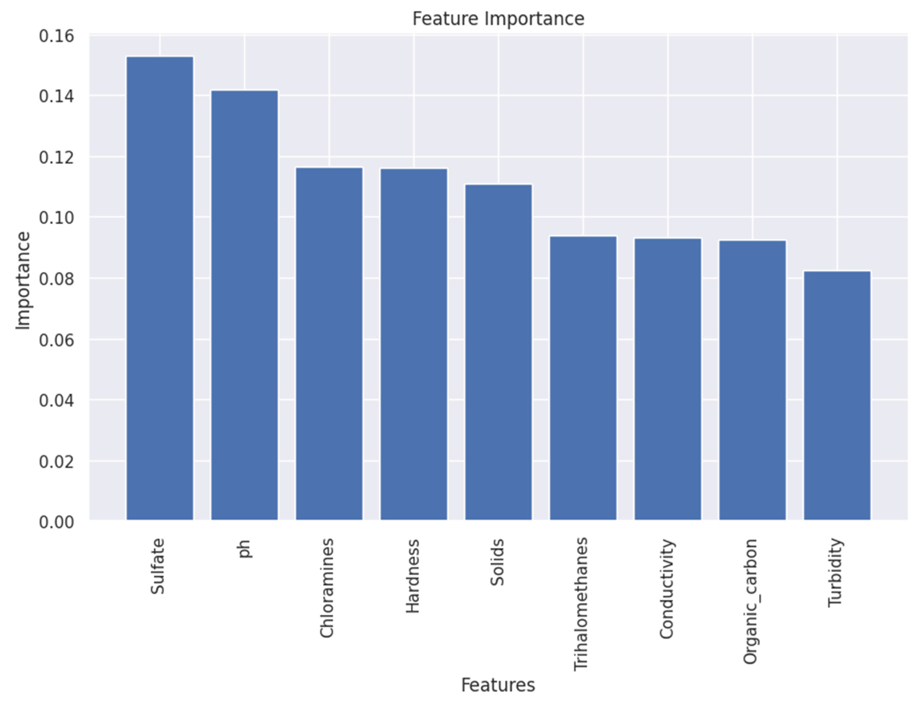
Based on the change in the model performance as a numerical indicator, the Permutation Feature Importance (PFI) technique was used to assess the influence of the features on the ML-based classification. The importance scores obtained from tree-based models, such as Random Forest or Gradient Boosting, are typically referred to as "Feature Importance." These scores represent the relative importance of each input feature in contributing to the model's predictive performance. The feature importance scores provide insights into which features have the most significant impact on the model's predictions. They can be used to identify the most influential features, prioritize feature selection or engineering efforts, and gain a better understanding of the underlying relationships between the features and the target variable. According to PFI analysis, compared to the other characteristics, sulphate has the most significance in predicting channel drinking water quality. To demonstrate the strong reaction of channel drinking water quality predicted from the ML-based classification model due to the change in the predictors, the significance scores are displayed in Figure 6. The pH, chloramines and hardness are the most significant features along with the sulphate. The shuffle signal of input series may result in the highest response in the change in feature importance scores.

4. Conclusion

In conclusion, this study focused on the application of machine learning classifiers for accurately predicting and classifying drinking water quality. The evaluation of various ML algorithms revealed that the XGBoost model achieved the highest accuracy among the classifiers. The prediction accuracy was further improved up to 3.5% through the use of Stacked Ensemble Classifiers (SEC). These findings suggest that XGBoost and the SEC hold promise can be used for decision support system to ensure the safety and sustainability of drinking water quality assessments.

Data Availability Statement

All relevant data are included in the paper or can be made available upon request from the corresponding author.

Conflicts of Interest

On behalf of all authors, the corresponding author stated that there is no conflict of interest.

References

  1. Derdour, A.; Jodar-Abellan, A.; Pardo, M.Á.; Ghoneim, S.S.M.; Hussein, E.E. Designing Efficient and Sustainable Predictions of Water Quality Indexes at the Regional Scale Using Machine Learning Algorithms. Water 2022, 14, 2801. [Google Scholar] [CrossRef]
  2. Panneerselvam, B.; Ravichandran, N.; Kaliyappan, S.P.; Karuppannan, S.; Bidorn, B. Quality and Health Risk Assessment of Groundwater for Drinking and Irrigation Purpose in Semi-Arid Region of India Using Entropy Water Quality and Statistical Techniques. Water 2023, 15, 601. [Google Scholar] [CrossRef]
  3. Adeloju, S.B.; Khan, S.; Patti, A.F. Arsenic Contamination of Groundwater and Its Implications for Drinking Water Quality and Human Health in Under-Developed Countries and Remote Communities—A Review. Appl. Sci. 2021, 11, 1926. [Google Scholar] [CrossRef]
  4. Shi, Z.; Chow, C.W.K.; Fabris, R.; Liu, J.; Jin, B. Applications of Online UV-Vis Spectrophotometer for Drinking Water Quality Monitoring and Process Control: A Review. Sensors 2022, 22, 2987. [Google Scholar] [CrossRef]
  5. Jung, Y.-J.; Khant, N.A.; Kim, H.; Namkoong, S. Impact of Climate Change on Waterborne Diseases: Directions towards Sustainability. Water 2023, 15, 1298. [Google Scholar] [CrossRef]
  6. Hussain, S.; Reza, M. Environmental Damage and Global Health: Understanding the Impacts and Proposing Mitigation Strategies. J. Big-Data Anal. Cloud Comput. 2023, 8, 1–21. [Google Scholar]
  7. Ongeri, S. Bacteriological Quality of Drinking Water in Administrative Wards around Kisii Town, Kisii County, Kenya. East Afr. J. Contemp. Res. 2023, 3, 27–37. [Google Scholar]
  8. Khosravi, M.; Ghoochani, S.; Nazemi, N. Deep Learning-Based Modeling of Daily Suspended Sediment Concentration and Discharge in Esopus Creek 2023.
  9. Water And Sanitation in Developing Countries: Including Health in the Equation. Environ. Sci. Technol. 2007, 41, 17–24. [CrossRef]
  10. Anik, A.H.; Sultan, M.B.; Alam, M.; Parvin, F.; Ali, M.M.; Tareq, S.M. The Impact of Climate Change on Water Resources and Associated Health Risks in Bangladesh: A Review. Water Secur. 2023, 18, 100133. [Google Scholar] [CrossRef]
  11. Rhue, S.J.; Torrico, G.; Amuzie, C.; Collins, S.M.; Lemaitre, A.; Workman, C.L.; Rosinger, A.Y.; Pearson, A.L.; Piperata, B.A.; Wutich, A.; et al. The Effects of Household Water Insecurity on Child Health and Well-Being. WIREs Water n/a. [CrossRef]
  12. García-Ávila, F.; Zhindón-Arévalo, C.; Valdiviezo-Gonzales, L.; Cadme-Galabay, M.; Gutiérrez-Ortega, H.; del Pino, L.F. A Comparative Study of Water Quality Using Two Quality Indices and a Risk Index in a Drinking Water Distribution Network. Environ. Technol. Rev. 2022, 11, 49–61. [Google Scholar] [CrossRef]
  13. Wyrwoll, P.R.; Manero, A.; Taylor, K.S.; Rose, E.; Quentin Grafton, R. Measuring the Gaps in Drinking Water Quality and Policy across Regional and Remote Australia. Npj Clean Water 2022, 5, 1–14. [Google Scholar] [CrossRef]
  14. Drinking-Water Available online:. Available online: https://www.who.int/news-room/fact-sheets/detail/drinking-water (accessed on 9 August 2023).
  15. Li, P.; Wu, J. Drinking Water Quality and Public Health. Expo. Health 2019, 11, 73–79. [Google Scholar] [CrossRef]
  16. Water Quality & Treatment: A Handbook on Drinking Water; Edzwald, J. K., American Water Works Association, Eds.; 6th ed.; McGraw-Hill: New York, 2011; ISBN 978-0-07-163011-5. [Google Scholar]
  17. Scanlon, B.R.; Fakhreddine, S.; Reedy, R.C.; Yang, Q.; Malito, J.G. Drivers of Spatiotemporal Variability in Drinking Water Quality in the United States. Environ. Sci. Technol. 2022, 56, 12965–12974. [Google Scholar] [CrossRef]
  18. Zhang, Z.-M.; Zhang, F.; Du, J.-L.; Chen, D.-C. Surface Water Quality Assessment and Contamination Source Identification Using Multivariate Statistical Techniques: A Case Study of the Nanxi River in the Taihu Watershed, China. Water 2022, 14, 778. [Google Scholar] [CrossRef]
  19. Yang, W.; Zhao, Y.; Wang, D.; Wu, H.; Lin, A.; He, L. Using Principal Components Analysis and IDW Interpolation to Determine Spatial and Temporal Changes of Surface Water Quality of Xin’anjiang River in Huangshan, China. Int. J. Environ. Res. Public. Health 2020, 17, 2942. [Google Scholar] [CrossRef] [PubMed]
  20. Ebrahimi, S.; Khorram, M. Variability Effect of Hydrological Regime on River Quality Pattern and Its Uncertainties: Case Study of Zarjoob River in Iran. J. Hydroinformatics 2021, 23, 1146–1164. [Google Scholar] [CrossRef]
  21. Ghoochani, S.; Salehi, M.; DeSimone, D.; Esfandarani, M.S.; Bhattacharjee, L. Studying the Impacts of Non-Routine Extended Schools’ Closure on Heavy Metal Release into Tap Water. Environ. Sci. Water Res. Technol. 2022, 8, 1223–1235. [Google Scholar] [CrossRef]
  22. Yusri, W.M.E.W.M.; Ramli, M.H.M.; Khusaini, N.S.; Mohamed, Z. IoT Based Water Quality Monitoring System and Test for Swimming Pool Water Physicochemical Quality. AIP Conf. Proc. 2023, 2609, 020002. [Google Scholar] [CrossRef]
  23. Water Quality Assessments|A Guide to the Use of Biota, Sediments And Available online:. Available online: https://www.taylorfrancis.com/books/mono/10.1201/9781003062103/water-quality-assessments-deborah-chapman (accessed on 9 August 2023).
  24. Samarinas, N.; Spiliotopoulos, M.; Tziolas, N.; Loukas, A. Synergistic Use of Earth Observation Driven Techniques to Support the Implementation of Water Framework Directive in Europe: A Review. Remote Sens. 2023, 15, 1983. [Google Scholar] [CrossRef]
  25. Uddin, M.G.; Nash, S.; Rahman, A.; Olbert, A.I. A Novel Approach for Estimating and Predicting Uncertainty in Water Quality Index Model Using Machine Learning Approaches. Water Res. 2023, 229, 119422. [Google Scholar] [CrossRef]
  26. Uddin, M.G.; Nash, S.; Rahman, A.; Olbert, A.I. Performance Analysis of the Water Quality Index Model for Predicting Water State Using Machine Learning Techniques. Process Saf. Environ. Prot. 2023, 169, 808–828. [Google Scholar] [CrossRef]
  27. Mehedi, M.A.A.; Khosravi, M.; Yazdan, M.M.S.; Shabanian, H. Exploring Temporal Dynamics of River Discharge Using Univariate Long Short-Term Memory (LSTM) Recurrent Neural Network at East Branch of Delaware River. Hydrology 2022, 9, 202. [Google Scholar] [CrossRef]
  28. Karimi, M.; Khosravi, M.; Fathollahi, R.; Khandakar, A.; Vaferi, B. Determination of the Heat Capacity of Cellulosic Biosamples Employing Diverse Machine Learning Approaches. Energy Sci. Eng. 2022, 10, 1925–1939. [Google Scholar] [CrossRef]
  29. Abdollahzadeh, M.; Khosravi, M.; Hajipour Khire Masjidi, B.; Samimi Behbahan, A.; Bagherzadeh, A.; Shahkar, A.; Tat Shahdost, F. Estimating the Density of Deep Eutectic Solvents Applying Supervised Machine Learning Techniques. Sci. Rep. 2022, 12, 4954. [Google Scholar] [CrossRef] [PubMed]
  30. Ibrahim, H.; Yaseen, Z.M.; Scholz, M.; Ali, M.; Gad, M.; Elsayed, S.; Khadr, M.; Hussein, H.; Ibrahim, H.H.; Eid, M.H.; et al. Evaluation and Prediction of Groundwater Quality for Irrigation Using an Integrated Water Quality Indices, Machine Learning Models and GIS Approaches: A Representative Case Study. Water 2023, 15, 694. [Google Scholar] [CrossRef]
  31. Ahmad, M.; Al Mehedi, M.A.; Yazdan, M.M.S.; Kumar, R. Development of Machine Learning Flood Model Using Artificial Neural Network (ANN) at Var River. Liquids 2022, 2, 147–160. [Google Scholar] [CrossRef]
  32. Mehedi, M.A.A.; Yazdan, M.M.S. Automated Particle Tracing & Sensitivity Analysis for Residence Time in a Saturated Subsurface Media. Liquids 2022, 2, 72–84. [Google Scholar] [CrossRef]
  33. Piazza, S.; Sambito, M.; Freni, G. Analysis of Optimal Sensor Placement in Looped Water Distribution Networks Using Different Water Quality Models. Water 2023, 15, 559. [Google Scholar] [CrossRef]
  34. Reljić, M.; Romić, M.; Romić, D.; Gilja, G.; Mornar, V.; Ondrasek, G.; Bubalo Kovačić, M.; Zovko, M. Advanced Continuous Monitoring System—Tools for Water Resource Management and Decision Support System in Salt Affected Delta. Agriculture 2023, 13, 369. [Google Scholar] [CrossRef]
  35. Younes, K.; Kharboutly, Y.; Antar, M.; Chaouk, H.; Obeid, E.; Mouhtady, O.; Abu-samha, M.; Halwani, J.; Murshid, N. Application of Unsupervised Machine Learning for the Evaluation of Aerogels’ Efficiency towards Ion Removal—A Principal Component Analysis (PCA) Approach. Gels 2023, 9, 304. [Google Scholar] [CrossRef]
  36. Zhou, Y.; Wang, X.; Li, W.; Zhou, S.; Jiang, L. Water Quality Evaluation and Pollution Source Apportionment of Surface Water in a Major City in Southeast China Using Multi-Statistical Analyses and Machine Learning Models. Int. J. Environ. Res. Public. Health 2023, 20, 881. [Google Scholar] [CrossRef]
  37. Yazdan, M.M.S.; Ahad, M.T.; Kumar, R.; Mehedi, M.A.A. Estimating Flooding at River Spree Floodplain Using HEC-RAS Simulation. J 2022, 5, 410–426. [Google Scholar] [CrossRef]
  38. Electronics | Free Full-Text | IoT-Enabled Chlorine Level Assessment and Prediction in Water Monitoring System Using Machine Learning Available online:. Available online: https://www.mdpi.com/2079-9292/12/6/1458 (accessed on 9 August 2023).
  39. Li, L.; Rong, S.; Wang, R.; Yu, S. Recent Advances in Artificial Intelligence and Machine Learning for Nonlinear Relationship Analysis and Process Control in Drinking Water Treatment: A Review. Chem. Eng. J. 2021, 405, 126673. [Google Scholar] [CrossRef]
  40. Taffese, W.Z.; Sistonen, E. Machine Learning for Durability and Service-Life Assessment of Reinforced Concrete Structures: Recent Advances and Future Directions. Autom. Constr. 2017, 77, 1–14. [Google Scholar] [CrossRef]
  41. A Transdisciplinary Review of Deep Learning Research and Its Relevance for Water Resources Scientists - Shen - 2018 - Water Resources Research - Wiley Online Library Available online:. Available online: https://agupubs.onlinelibrary.wiley.com/doi/10.1029/2018WR022643 (accessed on 9 August 2023).
  42. Mehedi, M.A.A.; Reichert, N.; Molkenthin, F. SENSITIVITY ANALYSIS OF HYPORHEIC EXCHANGE TO SMALL SCALE CHANGES IN GRAVEL-SAND FLUMEBED USING A COUPLED GROUNDWATER-SURFACE WATER MODEL. 2020.
  43. Vinuesa, R.; Azizpour, H.; Leite, I.; Balaam, M.; Dignum, V.; Domisch, S.; Felländer, A.; Langhans, S.D.; Tegmark, M.; Fuso Nerini, F. The Role of Artificial Intelligence in Achieving the Sustainable Development Goals. Nat. Commun. 2020, 11, 233. [Google Scholar] [CrossRef]
  44. Chen, K.; Chen, H.; Zhou, C.; Huang, Y.; Qi, X.; Shen, R.; Liu, F.; Zuo, M.; Zou, X.; Wang, J.; et al. Comparative Analysis of Surface Water Quality Prediction Performance and Identification of Key Water Parameters Using Different Machine Learning Models Based on Big Data. Water Res. 2020, 171, 115454. [Google Scholar] [CrossRef]
  45. Lashkaripour, A.; Rodriguez, C.; Mehdipour, N.; Mardian, R.; McIntyre, D.; Ortiz, L.; Campbell, J.; Densmore, D. Machine Learning Enables Design Automation of Microfluidic Flow-Focusing Droplet Generation. Nat. Commun. 2021, 12, 25. [Google Scholar] [CrossRef]
  46. Kumar, R.; Yazdan, M.M.S.; Mehedi, M.A.A. Demystifying the Preventive Measures for Flooding from Groundwater Triggered by the Rise in Adjacent River Stage. 2022. [CrossRef]
  47. Wasana, H.M.S.; Perera, G.D.R.K.; Gunawardena, P.D.S.; Fernando, P.S.; Bandara, J. WHO Water Quality Standards Vs Synergic Effect(s) of Fluoride, Heavy Metals and Hardness in Drinking Water on Kidney Tissues. Sci. Rep. 2017, 7, 42516. [Google Scholar] [CrossRef]
  48. Mehedi, M.A.A.; Yazdan, M.M.S.; Ahad, M.T.; Akatu, W.; Kumar, R.; Rahman, A. Quantifying Small-Scale Hyporheic Streamlines and Resident Time under Gravel-Sand Streambed Using a Coupled HEC-RAS and MIN3P Model. Eng 2022, 3, 276–300. [Google Scholar] [CrossRef]
  49. Damo, R.; Icka, P. Evaluation of Water Quality Index for Drinking Water. Pol. J. Environ. Stud. 2013. [Google Scholar]
  50. Han, X.; Liu, X.; Gao, D.; Ma, B.; Gao, X.; Cheng, M. Costs and Benefits of the Development Methods of Drinking Water Quality Index: A Systematic Review. Ecol. Indic. 2022, 144, 109501. [Google Scholar] [CrossRef]
  51. VanDerslice, J. Drinking Water Infrastructure and Environmental Disparities: Evidence and Methodological Considerations. Am. J. Public Health 2011, 101, S109–S114. [Google Scholar] [CrossRef]
  52. Adeniran, A.; Daniell, K.A.; Pittock, J. Water Infrastructure Development in Nigeria: Trend, Size, and Purpose. Water 2021, 13, 2416. [Google Scholar] [CrossRef]
  53. Hangan, A.; Chiru, C.-G.; Arsene, D.; Czako, Z.; Lisman, D.F.; Mocanu, M.; Pahontu, B.; Predescu, A.; Sebestyen, G. Advanced Techniques for Monitoring and Management of Urban Water Infrastructures—An Overview. Water 2022, 14, 2174. [Google Scholar] [CrossRef]
  54. Ramesh, N.I.; Davison, A.C. Local Models for Exploratory Analysis of Hydrological Extremes. J. Hydrol. 2002, 256, 106–119. [Google Scholar] [CrossRef]
  55. Khosravi, M.; Mehedi, M.A.A.; Baghalian, S.; Burns, M.; Welker, A.L.; Golub, M. Using Machine Learning to Improve Performance of a Low-Cost Real-Time Stormwater Control Measure 2022.
  56. Yazdan, M.M.S.; Khosravia, M.; Saki, S.; Mehedi, M.A.A. Forecasting Energy Consumption Time Series Using Recurrent Neural Network in Tensorflow 2022.
  57. Khosravi, M.; Arif, S.B.; Ghaseminejad, A.; Tohidi, H.; Shabanian, H. Performance Evaluation of Machine Learning Regressors for Estimating Real Estate House Prices 2022.
  58. Čeh, M.; Kilibarda, M.; Lisec, A.; Bajat, B. Estimating the Performance of Random Forest versus Multiple Regression for Predicting Prices of the Apartments. ISPRS Int. J. Geo-Inf. 2018, 7, 168. [Google Scholar] [CrossRef]
  59. Arumugam, S.R.; Gowr, S. ; Abimala; Balakrishna; Manoj, O. Performance Evaluation of Machine Learning and Deep Learning Techniques. In Convergence of Deep Learning In Cyber-IoT Systems and Security; John Wiley & Sons, Ltd, 2022; pp. 21–65 ISBN 978-1-119-85768-6.
  60. Miao, X.; Jiang, A.; Zhu, Y.; Kwan, H.K. A Joint Learning Framework for Gaussian Processes Regression and Graph Learning. Signal Process. 2022, 201, 108708. [Google Scholar] [CrossRef]
  61. Khosravi, M.; Tabasi, S.; Hossam Eldien, H.; Motahari, M.R.; Alizadeh, S.M. Evaluation and Prediction of the Rock Static and Dynamic Parameters. J. Appl. Geophys. 2022, 199, 104581. [Google Scholar] [CrossRef]
  62. Khosravi, M.; Duti, B.M.; Yazdan, M.M.S.; Ghoochani, S.; Nazemi, N.; Shabanian, H. Multivariate Multi-Step Long Short-Term Memory Neural Network for Simultaneous Stream-Water Variable Prediction. Eng 2023, 4, 1933–1950. [Google Scholar] [CrossRef]
  63. Prakaisak, I.; Wongchaisuwat, P. Hydrological Time Series Clustering: A Case Study of Telemetry Stations in Thailand. Water 2022, 14, 2095. [Google Scholar] [CrossRef]
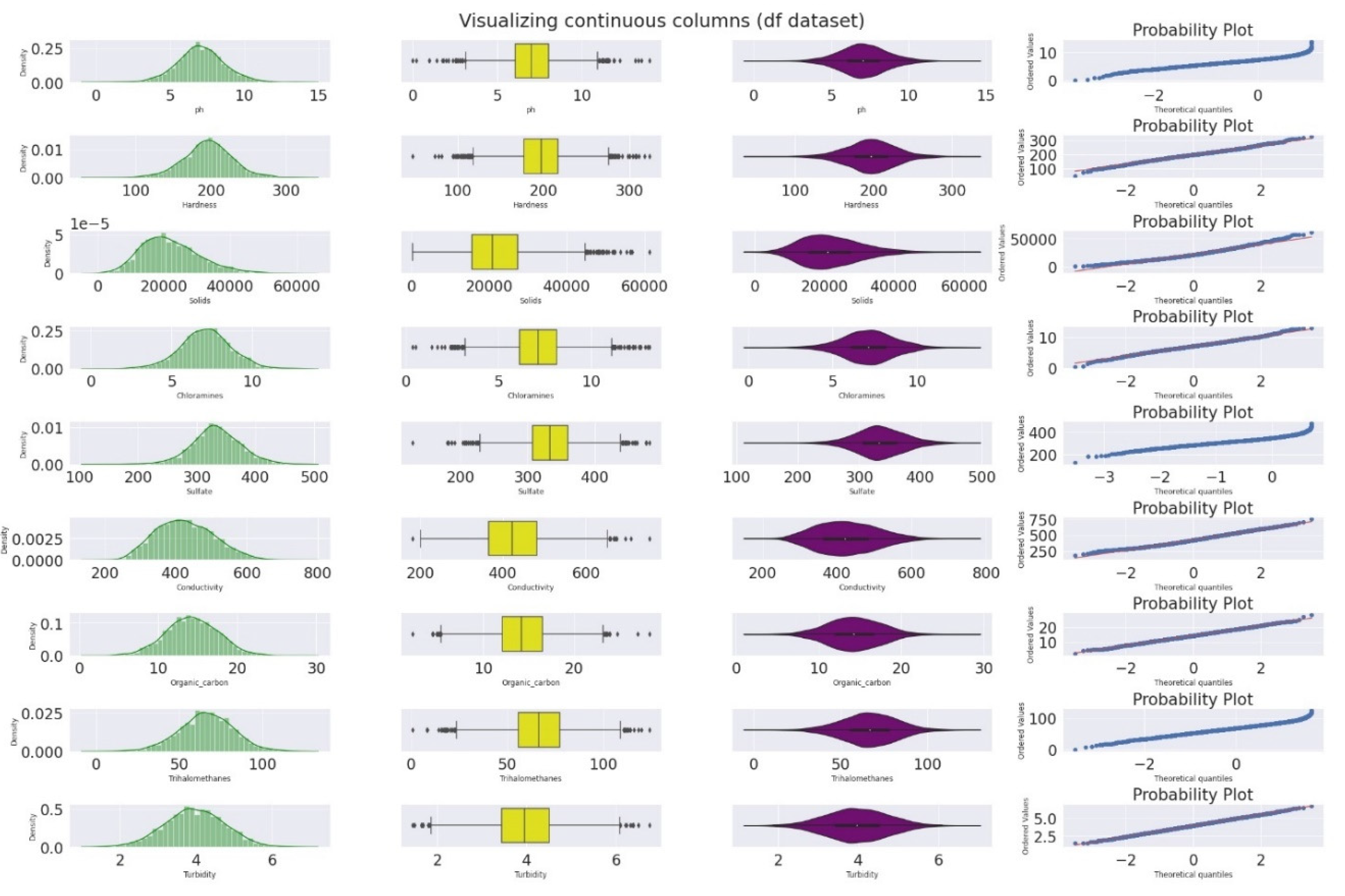
Figure 1. Distribution of the water quality variables.
Preprints 83007 g001
Figure 5. Confusion matrices show various model performances in detecting drinking water quality.
Preprints 83007 g004
Figure 6. Rank of input features according to their Feature Importance.
Preprints 83007 g005
Table 1. Full description of the input features.
Input features WHO limits
Ph 6.5–8.5
Hardness 200 mg/L
Solids 1000 ppm
Chloramines 4 ppm
Sulfate 1000 mg/L
Conductivity 400 μS/cm
Organic carbon 10 ppm
Trihalomethanes 80 ppm
Turbidity 5 NTU
Table 3. Performance comparison of ML classifiers.
Model F1-score Percentage (%) Jaccard
Logistic Regression (LR) 0.21 61.58 0.11
Support Vector Machine (SVR) 0.23 57.12 0.015
Stochastic Gradient Descent (SGD) 0.43 52.37 0.31
K-Nearest Neighbors (KNN) 0.49 63.24 0.32
Gaussian Process Classifiers (GPC) 0.59 73.36 0.39
Gaussian Naïve Bayes (GNB) 0.64 75.08 3.66
Decision Tree (DT) 0.91 83.61 0.87
Random Forest (RF) 0.93 85.37 0.89
Stacked Ensemble Classifier (SEC) 0.65 92.98 3.14
Extreme Gradient Boosting (XGboost) 0.91 89.47 2.15
Disclaimer/Publisher’s Note: The statements, opinions and data contained in all publications are solely those of the individual author(s) and contributor(s) and not of MDPI and/or the editor(s). MDPI and/or the editor(s) disclaim responsibility for any injury to people or property resulting from any ideas, methods, instructions or products referred to in the content.
Copyright: This open access article is published under a Creative Commons CC BY 4.0 license, which permit the free download, distribution, and reuse, provided that the author and preprint are cited in any reuse.
Prerpints.org logo

Preprints.org is a free preprint server supported by MDPI in Basel, Switzerland.

Subscribe

© 2024 MDPI (Basel, Switzerland) unless otherwise stated