
Submitted:
18 August 2023
Posted:
22 August 2023
You are already at the latest version
Abstract
Background: Electrical conductivity of trabecular bone at 100 kHz was recently reported as a good predictor of bone volume fraction. However, to quantify its relationship with the free water (or physiological solution) content and between the conductivities of its constituents, is still unclear. Methods: In this contribution, in silico models inspired by microCT images of trabecular bovine samples were used to build realistic geometries. Finite Element Method was applied to solve the electrical problem and to robustly fit the conductivity of the constituents with literature data. The obtained effective electrical conductivity was compared to Bruggeman three media mixture model: physiological solution, bone marrow and bone matrix. Results: The values for physiological solution plus bone marrow and bone matrix that captured better the bone volume fraction in the two media Finite Element model were: σps+bm = 298.4 mS/m and σb = 21.0 mS/m, respectively. Additionally, relative good results were obtained by a three media Bruggeman mixture model with σbm= 103 mS/m, σb= 21.0 mS/m, and σps= 1200 mS/m. Simple linear relationships between the proportions of constituents depending on bone volume fraction were tested. Degree of anisotropy and fractal dimension do not show detectable changes in effective conductivity. Conclusions: These results provided some useful findings for simulation purposes: first, a higher value of electrical conductivity of bone marrow has to be used in order to obtain similar values to those experimental published data. Second, anisotropy is not detectable by conductivity measurements for small trabecular samples (cube 5 mm). Finally, the simulations presented here showed a relatively good fitting of the mixture Bruggeman model which potentially would allow both, accounting for the free water content and re-scaling the model for whole bone electrical simulations.
Keywords:
computer model
; trabecular bone
; electrical conductivity
1. Introduction
The dielectric properties (DP) at low frequencies (< 1 MHz) are attractive biophysical parameters for technological medical applications, mainly, because their non ionizing condition and cheap implementation. Particularly for bone tissue, the DP has been used and proposed in: the evaluation of bone health [1], the monitoring of bone healing [2] and for bone growth stimulation [3,4]. Despite these very recent developments and advances, there is still a lack of knowledge on how certain factors affect the bone DP [5].
The bone is a hierarchical tissue and its structure is a complex matrix composed by several materials (collagen, water, minerals, marrow, etc. [6]) and structures (the macrostructure: trabecular or cancellous and cortical bone, the microstructure: Haversian systems, osteons, single trabeculae; continuing to the sub-microstructure, the nanostructure and the subnanostructure [7]). Most of these potential medical applications of DP implies the numerical simulation of the electromagnetic problem [1,8,9,10,11,12]. Then, there is an interest in modeling and quantifying the influence of both, composition and structure, on the DP [5,6,13,14,15]. For example, Balmer et al. measured and modeled at macro-scale the correlation of bovine bone micro-structure and electrical conductivity in physiological state [5]. They concluded that a linear model considering two media (solid matrix and bone marrow) captures the micro-structure (indirectly by the bone volume fraction, BV/TV). The authors proved that bone has a dominantly resistive behaviour and that any phase shift in the measurements are dominated by interface effects or due to stray capacitance. Consequently, the authors recommended, for a better interpretation, measuring at frequencies near to 100 kHz, whose phase shift is almost zero. The papers of Sierpowska et al. studied the correlation of dielectric properties and several parameters of trabecular bone in physiological state as well [16,17]. The authors concluded that the conductivity shows a strong dependence on water content, and that the interstitial bone marrow water has a major impact on overall trabecular bone conductivity. Additionally, they showed that fat and collagen content (the polarization effects on its surface associated with the hydration layer) correlated only with the relative permittivity at frequencies higher than 100 kHz. According to these references, at millimeter scale, it is valid the simplification of modeling the electric response of the trabecular bone by a two media material with their respective bone matrix conductivity () and bone marrow conductivity (). Simulation of such a material assumes that the conductivities of both components should be known and also its microstructure.
Computer simulation of the whole body electrical response (tenths/hundreds of centimeters) considering microstructural information is unaffordable. As an alternative, mixing theories from the effective medium theory has been used to homogenize the electrical properties of materials, which also allow model rescaling [18]. Wei et al. proposed a dielectric model considering fat, water content, and BV/TV on porcine non-physiological trabecular samples [13,14]. The authors proposed the unified mixing (UM) model [18] and obtained good results but unfortunately not applicable to in vivo conditions. Similar results using a three media Bruggeman mixture model were achieved by Ciuchi et al. but they only measured cortical porcine bone in non-physiological state as well [15]. The authors considered hydroxyapatite crystals, air, and the environment material was collagen. Smith and Foster proposed the Maxwell mixture model on low-water-content tissues [19] and Kosterich et al. applied the same model to bone cortical tissue [20].
This paper focused on the simulation of electrical conductivity of trabecular bone at 100 kHz and its relationship with micro-structure and free water. This frequency was selected in order to minimize interface and capacitance spurious effects and, consequently, the model was considered purely resistive. The geometries were inspired in microtomography images of bovine trabecular bone samples. The obtained model intends to capture information of both, micro-structure and water content by using mixed theory and finite element method (FEM) simulations. The objectives of this work were: to estimate the conductivity values of the constituents of a two media model (bone matrix and bone marrow); to evaluate a simple three media Bruggeman mixture model for considering the free water content of the sample; to predict potential sources of measurement errors. The procedure to do this was validated with experimental published data of bovine samples in physiological state. Once a confident model was obtained the following problems were analyzed: influence of the size of the sample and the anisotropy, and influence of washing process in sample preparation, which is related to fat and water content of bone marrow.
2. Materials and Methods
2.1. Sample preparation for building model geometries
The models simulated in this paper were inspired in real geometries of bovine trabecular bones obtained using micro Computed Tomography. Four cylindrical bovine trabecular bone samples (10 mm long, 16 mm diameter) were obtained from the femur head of two animals (A and B) from the local slaughterhouse within less than 24 hours post-mortem (stored at 4C). The samples were prepared using ad hoc tools: a handsaw made of two parallel blades and a hollow drill to extract cylinders. The marrow was removed from samples in order to obtain good contrast in the micro-CT images. The process started with an ultra-sonication in a 2% tergazyme solution using a B-220 Ultrasonicator (Branson Ultrasonics Americas, Danbury, CT, USA), and then cleaned under a gentle flow of distilled water. Micro-CT of the samples were measured using a Bruker SkyScan 1173 and microstructure parameters were computed using BoneJ [21].
The STL files (obtained from the Bruker SkyScan software) of the four samples were edited in order to obtain several geometry models from a single sample (see Figure 1). A total of 43 geometries were built. The 3D geometries were built from the filtered micro-CT images using the 3D Slicer software [22]. Two types of geometries were simulated: cylinders ( mm and mm, height and radius, respectively) and cubes ( mm), as it is shown in the Figure 1 (B) and (D), respectively. The size of the cylindrical model was selected to study the effect of BV/TV without being affected by the anisotropy (see [5]), while the cubic model was the maximum possible size. Image processing and meshing were performed using scikit-image [23], Meshlab [24], and Gmsh [25].
2.2. Modeling and computer simulations
2.2.1. Governing equations and boundary conditions
The models were based on the electric problem which was solved numerically using FEM implemented with FEniCS [26]. As the biological medium can be considered almost fully resistive at 100 kHz [5], the problem was approximated in its quasi-static form. Voltage was computed by the equation:
where is the conductivity of the materials ( and , for bone matrix and marrow, respectively). Electric field vector can be computed as . The power absorbed per unit tissue volume (also known as Specific Absorbed Ratio, SAR) can be calculated as SAR (dot product), being the current density vector. As the quasi-static approach was considered valid, SAR can be computed as SAR and was integrated over the sample volume, then obtaining the total power P. For the boundary conditions, active and dispersive electrodes were set at voltages and 0 V, respectively (see Figure 1 (B)). All the outer surfaces of the model (except that of the active and dispersive electrodes) were fixed to a null electric current. In order to obtain an effective conductivity , the power P was set equal to that obtained with a lumped resistor of length ℓ and area A (see Figure 1 (A)). That is,
2.2.2. Estimation of electrical conductivities
One of the cylindrical geometries (named model 0) was arbitrarily selected to obtain the conductivities of the constituent materials ( and ). In order to get different BV/TV values (from 0.2 to 0.6), an artificial procedure of trabeculae thinening was applied (similar to that presented in [27], see Figure 1(C)). Accounting for the BV/TV variable as independent, a series of simulations was carried out to minimize the difference between the obtained effective conductivity and the linear relationship proposed by Balmer et al. [5]. We applied four numerical experiments in which one of the components was left free and the other was fixed; and additionally, one simulation was carried out leaving both conductivities free. The minimization process was performed using the differential evolution optimization method [28]. For the validation of the results, the obtained values were used to simulate all the geometries.
2.2.3. Mixing theory
The mixture formula proposed in this work is the effective Bruggeman model [18]. The complex relative permittivity of a medium composed by N different materials is obtained by:
where and are the proportion and the complex relative permittivity of the material j, respectively. It is important to remark that and depend on the frequency, which is fixed at 100 kHz.
2.3. Tissue characteristics
In this section we reviewed the literature values of the considered components of trabecular bone: bone matrix and bone marrow. All the reviewed values were taken from bovine bone samples (as long as they are available) measured at frequencies around 100 kHz.
Kameo et al. have developed a mechanical poroelastic model of a single trabeculae using a porosity of 0.05 (BV/TV = 0.95) [29]. Cortical bone is a porous material, with values of BV/TV from 0.92 to 0.94 [5,30], therefore it is reasonable to simulate the bone matrix of the trabecular bone using the conductivity of cortical bone . Balmer et al. obtained 9.1 mS m[5]. One order of magnitude lower value was obtained by Unal et al. [30] ( 0.2 mS m), but they used distiled water to clean the samples. The review of Amin et al. shows values from 6.6 to 20.8 mS m [31].
Regarding the bone marrow, it is known that it varies its cellular composition according to the age of the individuals. For a young individual most of the marrow is red marrow, and for older ones the abundance of fat cells increases and the color of the marrow changes to yellow [32]. The results of Gabriel et al. shown values from 20 mSm to 100 mSm (values extrapolated from figures) for pigs of 10 kg to 250 kg and this can be explained by the water content (0.15 to 0.40), respectively. Samples of bone marrow from femurs and tibiae of 1 month old calves were measured in reference [19]. The volume fraction of water of the samples varied from 0.2 to 0.7, and conductivities from 200 mSm to 700 mS, respectively (values obtained from figures). Finally, the results presented in the ITIS database are 3.82 mS to 100 mS [33,34].
It is important to remark that free water hereafter will be indistinctly referred as physiological solution or porous water. We emphasized free water, because we are interested in the water that can flow freely within pores [35].
3. Results
3.1. Microstructure parameters
The cylindrical samples were used for studying the relationships between BV/TV and effective conductivity. The BV/TV mean (standard deviation) was 0.410 (0.07) with minimum and maximum values of 0.347 and 0.603, respectively. These samples were relatively smaller (2.5 mm) than the cubic samples (5 mm), and based on the reasoning of Balmer et al. [5], the importance of bone anisotropy increases when the bone region reaches an edge length of about 5 mm. In fact, the cube samples were used for evaluating the anisotropy and their results are summarized in Table 1. In addition to the BV/TV parameter, the degree of anisotropy (DA) and fractal dimenssion (FD) were computed by BoneJ software using the algorithms presented in [36].
3.2. Estimation of effective electrical conductivity by FEM
The results of the general procedure described in subSection 2.2.2 are summarized in Table 2. For example, in simulation #1 the differential evolution algorithm searched by varying the between 20 and 700 mS/m while the matrix conductivity was fixed at 9.1 mS/m.
Figure 2 shows the the estimation of the effective electrical conductivity using the results with minimum residues: simulation # 1 and # 5. It should be remarked that the estimation was performed with Sample 0 and the validation with Samples A and B.
3.3. Mixture models
The values that captured better the BV/TV variable in the two media FEM model were: = 21.0 mS/m and = 298.4 mS/m. One question that arises is which amount of free water is involved in the bone marrow value. We considered that no free water is inside the bone matrix (or its free water content is relatively constant). The simplest mixture model that can be tested is the Maxwell-Garnett [18]. If we consider only the marrow, we have to achieve an effective conductivity of 298.4 mS/m. Taking for the physiological solution = 78.0 and = 1200 mS/m and for the bone marrow (without free water) the values from database [33], then the proportions of water obtained were: 0.97 and 0.49, for yellow and red marrow, respectively. These values are not consistent with that presented in literature [35] which are around 20%. Therefore, other approach that can be evaluated is the Bruggeman model. The results presented next were computed using a three materials (, in Eq. 3): physiological solution, bone matrix, and bone marrow (without free water), 1,2 and 3, respectively. Note that in Eq. 3 the proportion, the relative permittivity and conductivity of each material are needed. The model tested is set as follows. The water proportion was defined as variable, and the bone matrix proportion () was varied from 0.2 to 0.6, which was approximately the range of the BV/TV of the samples of this work and [5]. Once and were fixed the other was determined . The values of the relative permittivity for the bone matrix and marrow (without water) were 2.28×10 and 1.73×10 (values from database [33]), respectively. Figure 3 (A) shows the results when values of conductivities were 20.8 mS/m and 103 mS/m. Two values for proportion of free water were evaluated 0.1 and 0.3. Figure 3 (B) shows the result when the conductivities proposed by Balmer et al. [5] were used ( 9.1 mS/m and 230.0 mS/m).
Figure 3 also shows the results of the Bruggeman model when the water content depends linearly on the BV/TV: , that is, the lower BV/TV the higher the water content. The reasoning followed to get A and B was to satisfy 0.2, 0.3 and 0.95 (porosity of cortical bone, [29]), 0.05 (free water content of cortical bone, [37]).
3.4. Prediction of potential sources of measurement errors
3.4.1. Anitsotropy
Cube geometries ( mm) were used in order to check whether the anisotropy can be detected by electrical measurements in such small samples. Figure 4 (A), (B) and (C) show the three types of simulation computed for each sample from Table 1. The results for these three simulations were three different effective conductivities. The ratio of the maximum and minimum value were computed and plotted against the degree of anisotropy and the fractal dimension (see Figure 4 (D) and (E)). The minimum square linear estimation was plotted as a guide.
A difference of 0.1 in degree of anisotropy resulted in approximately 10 % of conductivity ratio, and this was the greater difference detected with these models. No concluding results were obtained with the fractal dimension.
3.4.2. Influence of washing the samples
Generally, during the cutting process of the samples they are spraying with physiological solution (or similar) to prevent loss of moisture. Usually, after preparation, the samples are immersed in physiological solution and frozen and finally thawed just prior to measurements. Saha and Williams prevented that electrical properties of cortical bone can be affected by the described process [38]. In this section we simulated the diffusion of physiological solution inside the porous of the bone matrix. We selected the geometry of model 0 and the spatial distribution of the conductivity of the porous space was modeled with a Gaussian shape that smoothly goes from = 298.4 mS/m (in the center of the sample) to = 1200 mS/m (on the outer surface). The function when the sample was centered at the origin, was:
and with the parameter d, we simulated a deeper diffusion inside the matrix. Figure 5 shows the results of 35 simulations varying the parameter d from 0 to 5 mm. The percentage value of the conductivity with respect to the base value (when d tends to infinity) is plotted in Figure 5 (B). Note that, even with a d = 4 mm, the overestimation of the conductivity is 25% or greater.
4. Discussion
The results of this paper were focused on the electrical conductivity of trabecular bone at 100 kHz. At this frequency, there is a consensus in literature that indicates that the bone can be considered as a purely resistive media because the phase shift is almost zero [5,14,17]. Considering this, we have studied the role of micro-structure and physiological solution (or free water that can flow within the pores) in the effective electrical conductivity of samples.
The experiments of Balmer et al. (at 100 kHz, [5]) arrived to a linear relationship between BV/TV and the effective electrical conductivity of bone in physiological state. These experiments were performed with samples of cortical and trabecular bone, with mean BV/TV of 0.92 and 0.53, respectively. The authors also proposed values for the bone matrix and the bone marrow based on a simple two resistors in a parallel circuit, with 230 mS/m and 9.1 mS/m, respectively. These values are different from that extensively used in the bibliography [34], 103 mS/m (red bone marrow), 3.82 mS/m (yellow bone marrow) and 20.8 mS/m. On the other hand, the compilation of Gabriel and coauthors indicates that the effective electrical conductivity of trabecular (cancellous) bone is around 83.9 mS/m, which has some sense if the marrow is "red" but not when it is "yellow" (see the compiled information in [33]). Unfortunately, in this compilation, there is no information about the micro-structure of the trabecular bone. In the computer results presented here, using realistic micro-structure geometries, we obtained the values 300 mS/m and 21 mS/m for marrow and matrix, respectively. These values were robustly validated using independent geometries. The bone matrix value agreed well with that presented by Gabriel compilation for cortical bone but doubles that of Balmer and coworkers. Regarding the bone marrow, a much higher value was obtained, which is more similar to the values presented by Smith and Foster [19]. These results show that, a simple model of two resistors in parallel [5] is not enough to capture the BV/TV and both, matrix and marrow electrical conductivities.
The reasoning commented above evidences that 21 mS/m is a good enough value for the bone matrix (at least for computer simulation considering micro-structure) and, hopefully, it can be considered relatively constant with the free water content. Regarding the bone marrow, the problem is more difficult and the proportion of free water is not clearly known. Wei and collaborators measured volume fraction of water on porcine trabecular bone fitting a Unified mixing dielectric model but they obtained confusing results [14]. Instead of volume fraction the authors considered mass fraction, arriving to mean values from 0.13 to 0.18, when the BV/TV was between 0.29 and 0.40. The work of Smith and Foster [19] considered effective Maxwell mixture model and they measured volume fractions of water directly in the bone marrow, with values from 0.2 to 0.7. If BV/TV is around 0.4 then the bone marrow plus free water is 1-0.4 = 0.6 and 0.6×0.2 ≈ 0.12 and 0.6×0.7 ≈ 0.42, for the lowest and highest values of volume fraction of water in bone marrow [19], respectively. The work of Sierpowska et al. has shown that at 100 kHz the free water strongly affects the electrical conductivity of human trabecular bones and that it is mostly governed by the water inside the porous [16] but no information about the water volume fraction was given. Concluding, any value from 0.1 to 0.5 covers the range of the mentioned references for the water volume fraction. The results presented in this paper using the Bruggeman model are in line with water volume fraction from 0.2 to 0.3 for trabecular bone. The best model for representing effective electrical conductivity of the the cortical bone as well was obtained using the values of reference [33] (see Figure 3 (A)). It should be remarked that this is true when free water volume fraction has a negative linear relationship with BV/TV (in Figure 3 the curve called "linear"), which can be interpreted as the more porous matrix the easier the free water flows into the matrix. Therefore for a wide range from 0.2 to 0.95 of BV/TV and for physiological solution content varying linearly with it from 0.05 to 0.3 we arrived to:
where is the volume fraction of marrow, BV/TV and is the free water volume fraction. Consequently, the Bruggeman model using 103 mS/m, 21 mS/m, and 1200 mS/m for material 1, 2, and 3, respectively, represented relatively well the effective electrical conductivity of bone (cortical and trabecular) at 100 kHz and can be a good candidate for simulation purposes. Logically, this is a simplistic reasoning and certain limitations should be mentioned, like for example the composition according to the age of the individuals. For a young individual most of the marrow is red marrow, and more conductive (more free water) values are expected. On the other hand for older ones the abundance of fat would give lower values of conductivity.
Balmer et al. [5] commented that the importance of bone anisotropy increases when the bone region reaches an edge length of about 5 mm. To study this, we simulated cubic samples of such a size comparing the electrical conductivity with two parameters: degree of anisotropy and fractal dimension. We found no relevant information with the latter. Regarding the former, even differences between samples were captured by the variation of conductivity (which is around 10%), it certainly can be masked by measurement error. For example, Balmer and cohautors informed a root-mean-square (RMS) error of 31 mS/m for trabecular bone which in a 100 mS/m conductivity represents the 30 %.
During washing and storing of samples, the physiological solution could flows inside the porous of the bone matrix. Quantifying how this effect affects the electrical conductivity experimentally is very difficult. We have intended to emulate it by varying the bone marrow conductivity with the coordinates: at the center of the sample, we assigned 103 mS/m growing to 1200 mS/m in a Gaussian shape til reach the border of the sample. For example, if the parameter d = 4 mm, at the border of the sample a value of approximately 650 mS/m is reached, the overestimation of the effective conductivity is around 25% (Figure 5 (B)). Then, for dielectric properties measurements, it is really important to carefully design a protocol in order to minimize the washing and storing time with liquid phase of physiological solution.
5. Conclusions
The low frequency electrical conductivity of bone depends strongly from its micro-structure and water content. The in silico 3D models at 100 kHz inspired in microCT images of bovine samples demonstrates two important things: first, a higher value of electrical conductivity of bone marrow has to be used in order to obtain similar values to those experimental published data. Second, anisotropy is not detectable by conductivity measurement for small trabecular samples (cube 5 mm). The simulations were also used to fit the mixture Bruggeman model which potentially would allow both, accounting for the free water content and re-scaling the model for whole bone electrical simulations.
Author Contributions
Conceptualization, A.G-S, C.M.C. and R.M.I.; methodology, M.J.C. and L.O.B.; software R.M.I. and C.M.C.; formal analysis, A.G-S.; writing—original draft preparation, M.J.C., L.O.B., and R.M.I.; writing—review and editing, A.G-S. and C.M.C; funding acquisition, R.M.I and C.M.C. All authors have read and agreed to the published version of the manuscript.
Funding
This research work was granted by PICT 2020-SERIEA-00457 (Agencia Nacional de Promoción de la Investigación, el Desarrollo Tecnológico) and by Grant No. PUE 2018 229 20180100010 CO (CONICET).
Acknowledgments
M.J.C., R.M.I. and C.M.C. are thankful for the financial support from CONICET (Grant No. PUE 2018 229 20180100010 CO). We are also thankful for the experimental support of Dr. Martín Sánchez and Dr. Mariano Cipollone from YPF Tecnología (Y-TEC).
Conflicts of Interest
The authors declare no conflict of interest.
References
- Kimel-Naor, S.; Abboud, S.; Arad, M. Parametric electrical impedance tomography for measuring bone mineral density in the pelvis using a computational model. Medical Engineering & Physics 2016, 38, 701–707. [Google Scholar]
- Lin, M.C.; Hu, D.; Marmor, M.; Herfat, S.T.; Bahney, C.S.; Maharbiz, M.M. Smart bone plates can monitor fracture healing. Scientific reports 2019, 9, 1–15. [Google Scholar] [CrossRef]
- Khalifeh, J.M.; Zohny, Z.; MacEwan, M.; Stephen, M.; Johnston, W.; Gamble, P.; Zeng, Y.; Yan, Y.; Ray, W.Z. Electrical stimulation and bone healing: A review of current technology and clinical applications. IEEE reviews in biomedical engineering 2018, 11, 217–232. [Google Scholar] [CrossRef]
- Ramos, A.; Dos Santos, M.P.S. Capacitive stimulation-sensing system for instrumented bone implants: Finite element model to predict the electric stimuli delivered to the interface. Computers in Biology and Medicine 2023, 154, 106542. [Google Scholar] [CrossRef]
- Balmer, T.W.; Vesztergom, S.; Broekmann, P.; Stahel, A.; Büchler, P. Characterization of the electrical conductivity of bone and its correlation to osseous structure. Scientific reports 2018, 8, 1–8. [Google Scholar] [CrossRef]
- Sierpowska, J.; Lammi, M.; Hakulinen, M.; Jurvelin, J.; Lappalainen, R.; Töyräs, J. Effect of human trabecular bone composition on its electrical properties. Medical engineering & physics 2007, 29, 845–852. [Google Scholar]
- Rho, J.Y.; Kuhn-Spearing, L.; Zioupos, P. Mechanical properties and the hierarchical structure of bone. Medical engineering & physics 1998, 20, 92–102. [Google Scholar]
- Ron, A.; Abboud, S.; Arad, M. Home monitoring of bone density in the wrist—a parametric EIT computer modeling study. Biomedical Physics & Engineering Express 2016, 2, 035002. [Google Scholar]
- Wong, P.; George, S.; Tran, P.; Sue, A.; Carter, P.; Li, Q. Development and validation of a high-fidelity finite-element model of monopolar stimulation in the implanted guinea pig cochlea. IEEE Transactions on Biomedical Engineering 2015, 63, 188–198. [Google Scholar] [CrossRef]
- Zimmermann, U.; Ebner, C.; Su, Y.; Bender, T.; Bansod, Y.D.; Mittelmeier, W.; Bader, R.; van Rienen, U. Numerical simulation of electric field distribution around an instrumented total hip stem. Applied Sciences 2021, 11, 6677. [Google Scholar] [CrossRef]
- Feng, C.; Yao, J.; Wang, L.; Zhang, X.; Fan, Y. Idealized conductance: A new method to evaluate stiffness of trabecular bone. International Journal for Numerical Methods in Biomedical Engineering 2021, 37, e3425. [Google Scholar] [CrossRef] [PubMed]
- Blaszczyk, M.; Hackl, K. Multiscale modeling of cancellous bone considering full coupling of mechanical, electric and magnetic effects. Biomechanics and Modeling in Mechanobiology 2022, 21, 163–187. [Google Scholar] [CrossRef] [PubMed]
- Wei, W.; Shi, F.; Kolb, J. Impedimetric Analysis of Trabecular Bone Based on Cole and Linear Discriminant Analysis. Frontiers in Physics 2020, 8, 662. [Google Scholar] [CrossRef]
- Wei, W.; Shi, F.; Zhuang, J.; Kolb, J.F. Comprehensive characterization of osseous tissues from impedance measurements by effective medium approximation. AIP Advances 2021, 11, 105316. [Google Scholar] [CrossRef]
- Ciuchi, I.V.; Olariu, C.S.; Mitoseriu, L. Determination of bone mineral volume fraction using impedance analysis and Bruggeman model. Materials Science and Engineering: B 2013, 178, 1296–1302. [Google Scholar] [CrossRef]
- Sierpowska, J.; Hakulinen, M.; Töyräs, J.; Day, J.; Weinans, H.; Kiviranta, I.; Jurvelin, J.; Lappalainen, R. Interrelationships between electrical properties and microstructure of human trabecular bone. Physics in Medicine & Biology 2006, 51, 5289. [Google Scholar]
- Sierpowska, J.; Töyräs, J.; Hakulinen, M.; Saarakkala, S.; Jurvelin, J.; Lappalainen, R. Electrical and dielectric properties of bovine trabecular bone—relationships with mechanical properties and mineral density. Physics in Medicine & Biology 2003, 48, 775. [Google Scholar]
- Sihvola, A.H. Electromagnetic mixing formulas and applications; Number 47, Iet, 1999.
- Smith, S.R.; Foster, K.R. Dielectric properties of low-water-content tissues. Physics in Medicine & Biology 1985, 30, 965. [Google Scholar]
- Kosterich, J.D.; Foster, K.R.; Pollack, S.R. Dielectric permittivity and electrical conductivity of fluid saturated bone. IEEE Transactions on biomedical engineering 1983, pp. 81–86.
- Domander, R.; Felder, A.; Doube, M. BoneJ2 - refactoring established research software [version 2; peer review: 3 approved]. Wellcome Open Research 2021, 6. [Google Scholar] [CrossRef]
- Fedorov, A.; Beichel, R.; Kalpathy-Cramer, J.; Finet, J.; Fillion-Robin, J.C.; Pujol, S.; Bauer, C.; Jennings, D.; Fennessy, F.; Sonka, M.; et al. 3D Slicer as an image computing platform for the Quantitative Imaging Network. Magnetic resonance imaging 2012, 30, 1323–1341. [Google Scholar] [CrossRef]
- van der Walt, S.; Schönberger, J.L.; Nunez-Iglesias, J.; Boulogne, F.; Warner, J.D.; Yager, N.; Gouillart, E.; Yu, T.; the scikit-image contributors. scikit-image: Image processing in Python. PeerJ 2014, 2, e453. [Google Scholar] [CrossRef] [PubMed]
- Cignoni, P.; Callieri, M.; Corsini, M.; Dellepiane, M.; Ganovelli, F.; Ranzuglia, G. MeshLab: An Open-Source Mesh Processing Tool. In Proceedings of the Eurographics Italian Chapter Conference; Scarano, V.; Chiara, R.D.; Erra, U., Eds. The Eurographics Association, 2008. [CrossRef]
- Geuzaine, C.; Remacle, J.F. Gmsh: A 3-D finite element mesh generator with built-in pre-and post-processing facilities. International journal for numerical methods in engineering 2009, 79, 1309–1331. [Google Scholar] [CrossRef]
- Langtangen, H.P.; Logg, A. Solving PDEs in Python; Springer, 2017. [CrossRef]
- Irastorza, R.M.; Blangino, E.; Carlevaro, C.M.; Vericat, F. Modeling of the dielectric properties of trabecular bone samples at microwave frequency. Medical & biological engineering & computing 2014, 52, 439–447. [Google Scholar]
- Storn, R.; Price, K. Differential evolution–a simple and efficient heuristic for global optimization over continuous spaces. Journal of global optimization 1997, 11, 341–359. [Google Scholar] [CrossRef]
- Kameo, Y.; Ootao, Y.; Ishihara, M. Poroelastic analysis of interstitial fluid flow in a single lamellar trabecula subjected to cyclic loading. Biomechanics and modeling in mechanobiology 2016, 15, 361–370. [Google Scholar] [CrossRef] [PubMed]
- Unal, M.; Cingoz, F.; Bagcioglu, C.; Sozer, Y.; Akkus, O. Interrelationships between electrical, mechanical and hydration properties of cortical bone. Journal of the mechanical behavior of biomedical materials 2018, 77, 12–23. [Google Scholar] [CrossRef]
- Amin, B.; Elahi, M.A.; Shahzad, A.; Porter, E.; O’Halloran, M. A review of the dielectric properties of the bone for low frequency medical technologies. Biomedical Physics & Engineering Express 2019, 5, 022001. [Google Scholar]
- Gabriel, C.; Peyman, A. Dielectric properties of biological tissues; variation with age. Conn’s Handbook of Models for Human Aging 2018, pp. 939–952.
- Hasgall, P.; Di Gennaro, F.; Baumgartner, C.; Neufeld, E.; Gosselin, M.; Payne, D.; Klingenböck, A.; Kuster, N. Itis database for thermal and electromagnetic parameters of biological tissues, version 3.0, 2015.
- Gabriel, C. Compilation of the dielectric properties of body tissues at RF and microwave frequencies. Technical report, King’s Coll London (United Kingdom) Dept of Physics, 1996.
- Surowiec, R.K.; Allen, M.R.; Wallace, J.M. Bone hydration: How we can evaluate it, what can it tell us, and is it an effective therapeutic target? Bone reports 2022, 16, 101161. [Google Scholar] [CrossRef]
- Domander, R.; Felder, A.A.; Doube, M. BoneJ2-refactoring established research software. Wellcome Open Research 2021, 6. [Google Scholar] [CrossRef]
- Abbasi-Rad, S.; Akbari, A.; Malekzadeh, M.; Shahgholi, M.; Arabalibeik, H.; Rad, H.S. Quantifying cortical bone free water using short echo time (STE-MRI) at 1.5 T. Magnetic resonance imaging 2020, 71, 17–24. [Google Scholar] [CrossRef]
- Saha, S.; Williams, P. Effect of various storage methods on the dielectric properties of compact bone. Medical and Biological Engineering and Computing 1988, 26, 199–202. [Google Scholar] [CrossRef] [PubMed]
Figure 1.
The models geometries. (A) MicroCT slice image. (B) Cylindrical sample (model 0) and (C) artificial procedure of trabeculae thinening for the procedure to obtain the effective electrical conductivities. (D) Cubic sample to study the anisotropy effects.
Figure 1.
The models geometries. (A) MicroCT slice image. (B) Cylindrical sample (model 0) and (C) artificial procedure of trabeculae thinening for the procedure to obtain the effective electrical conductivities. (D) Cubic sample to study the anisotropy effects.
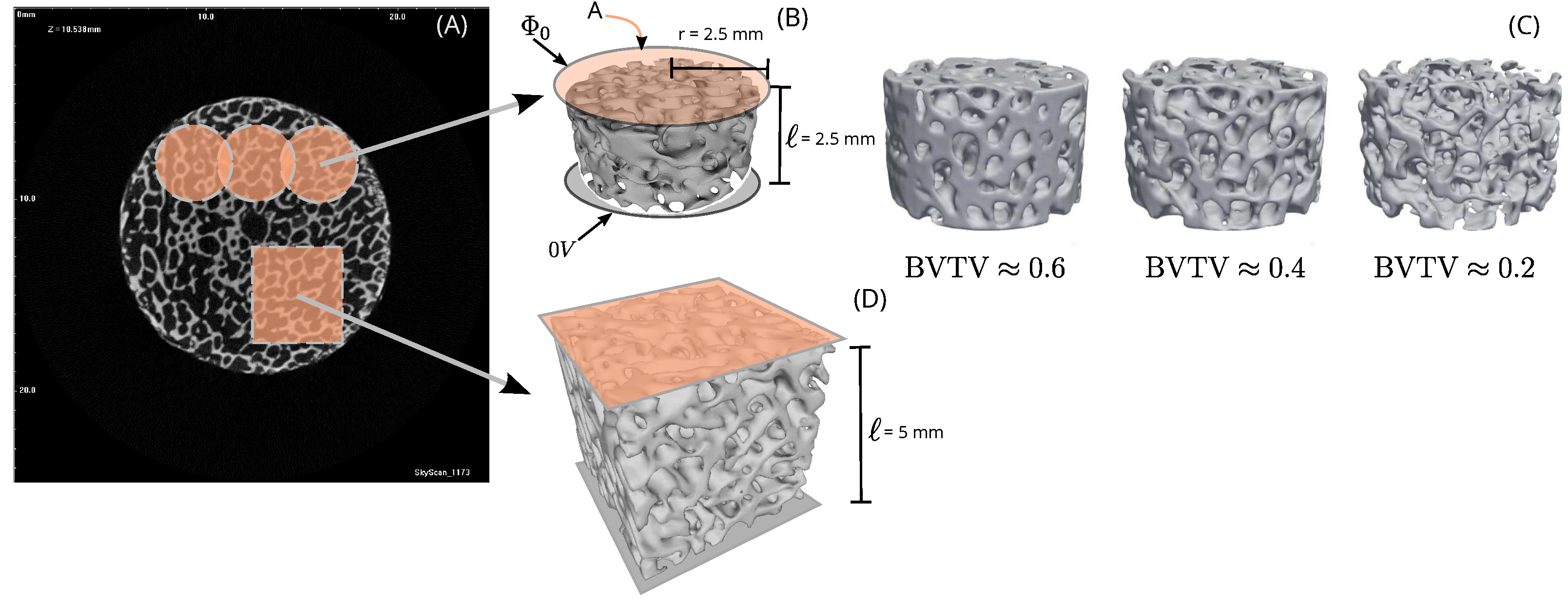
Figure 2.
Results on estimating the effective electrical conductivity. Simulation of all samples using (A) simulation # 1, fixing the conductivity of the bone matrix (B) simulation # 5, moving both, conductivity of bone matrix and bone marrow.
Figure 2.
Results on estimating the effective electrical conductivity. Simulation of all samples using (A) simulation # 1, fixing the conductivity of the bone matrix (B) simulation # 5, moving both, conductivity of bone matrix and bone marrow.
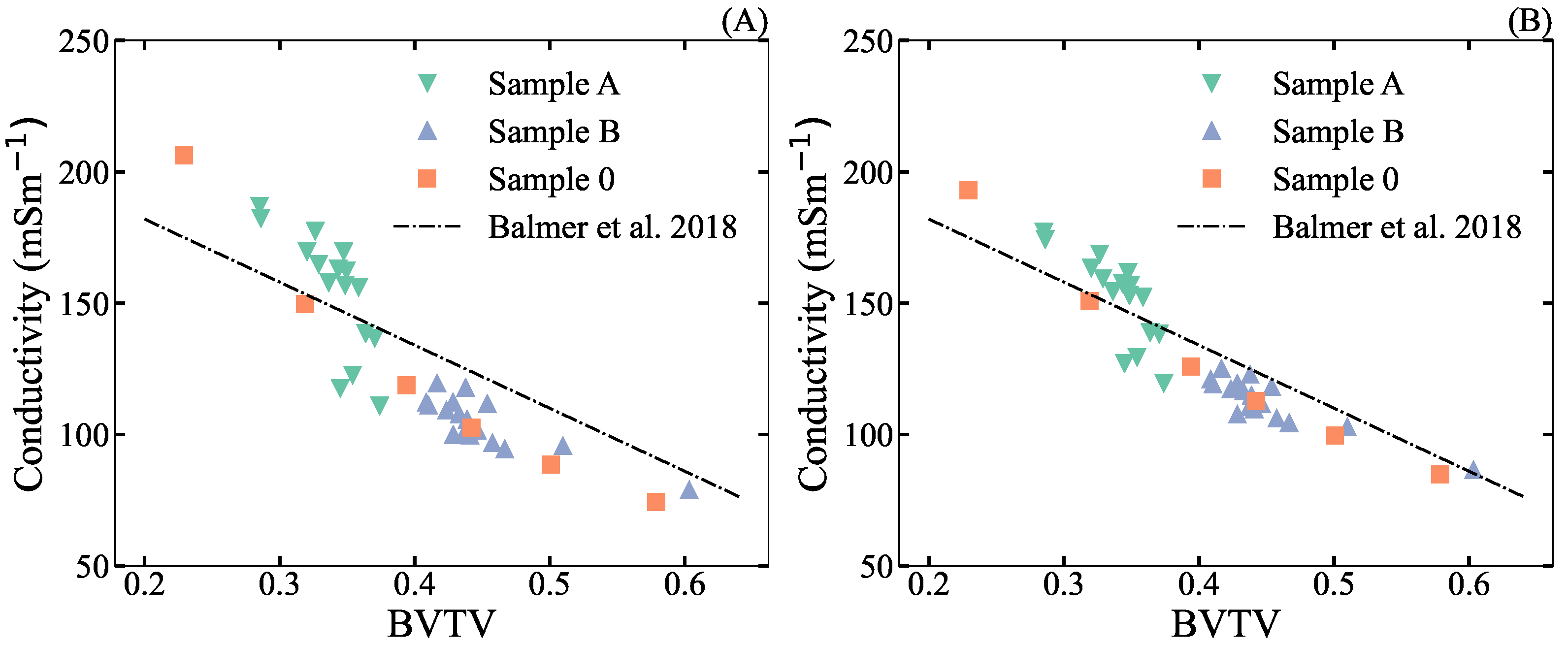
Figure 3.
Results of mixture models (Bruggeman model with 3 using two proportions of free water and a linear relationship between proportion of free water and BV/TV) compared to effective conductivity computed by simulation using FEM (same as Figure 2). The Balmer et al. linear relationship (dashed-dotted line) and experimental data (circle and +, trabecular and cortical) are also shown (data extracted from figures of [5]). (A) Values of reference [33] were used for porous and matrix (cortical bone and red marrow, respectively). (B) Values proposed by [5] were used.

Figure 4.
Study of anisotropy in cube samples. From (A) to (C) three measurement experiment models where the same sample is measured in the three directions. (D) and (E) show the ratio of the maximum and minimum effective conductivity and the degree of anisotropy (DA) and the fractal dimension (FD), respectively.
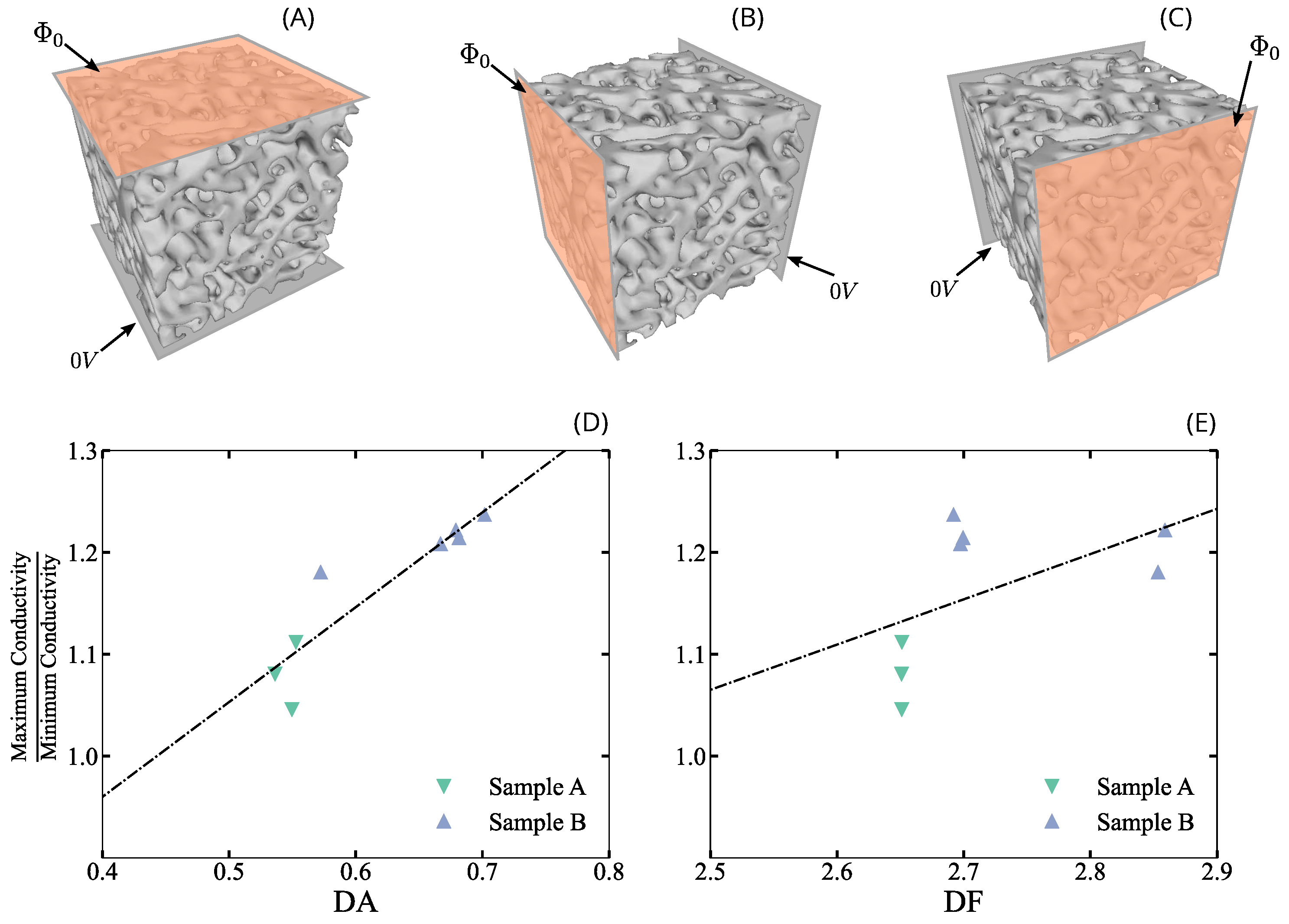
Figure 5.
Physiological solution diffusion inside the porous bone matrix. (A) Example of the conductivity map in the 3D geometry, the conductivity of the porous space was defined with Ec. 4. (B) Percent effective conductivity in function of the parameter d.
Figure 5.
Physiological solution diffusion inside the porous bone matrix. (A) Example of the conductivity map in the 3D geometry, the conductivity of the porous space was defined with Ec. 4. (B) Percent effective conductivity in function of the parameter d.
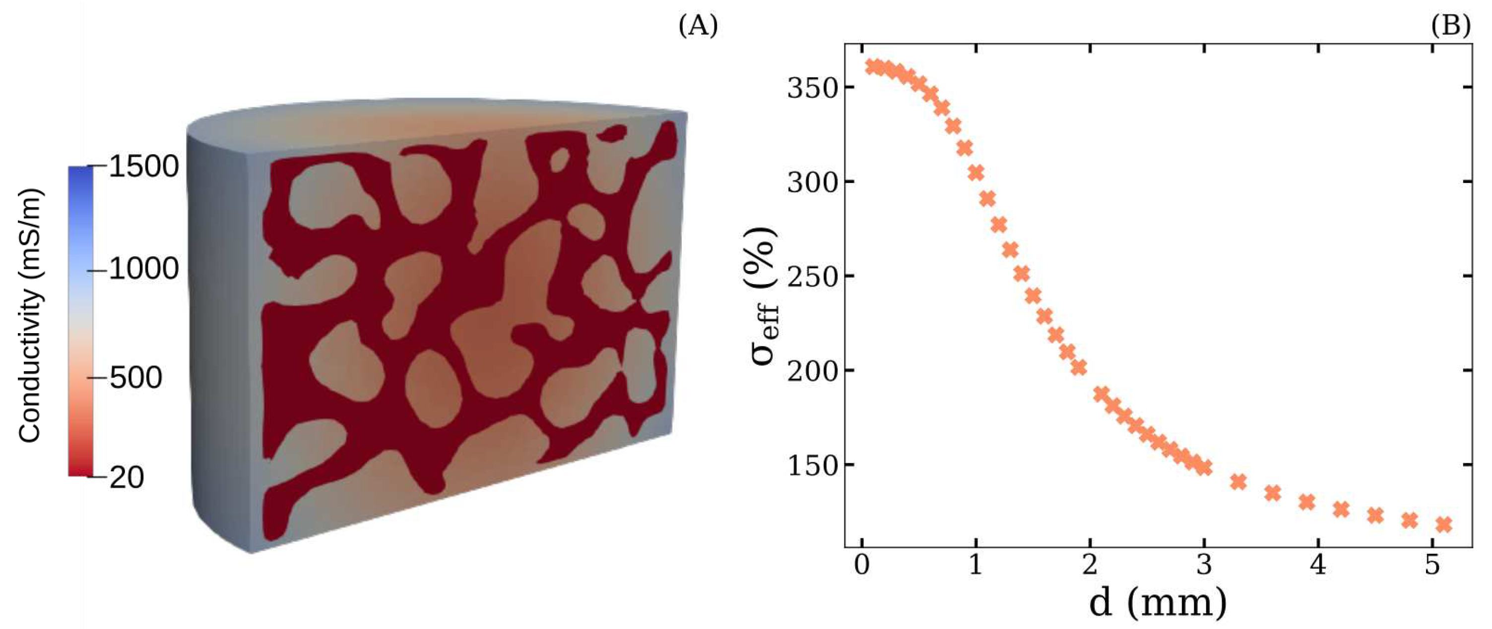

Table 1.
Microstructure properties of cubic samples.
| Sample | BV/TV | DA | FD |
|---|---|---|---|
| # 1 A | 0.348 | 0.536 | 2.651 |
| # 2 A | 0.339 | 0.549 | 2.651 |
| # 3 A | 0.419 | 0.553 | 2.651 |
| # 1 B | 0.473 | 0.679 | 2.859 |
| # 2 B | 0.515 | 0.572 | 2.853 |
| # 3 B | 0.485 | 0.681 | 2.699 |
| # 4 B | 0.460 | 0.702 | 2.692 |
| # 5 B | 0.447 | 0.667 | 2.697 |
Table 2.
Simulation plan and results of two media model of cylindrical samples.
| Range (mS/m) | Results (mS/m) | |||||
| Simulation | Residue | Reference | ||||
| # 1 | 20 -700 | 9.1 | 344.8 | 9.1 | 0.050 | [5] |
| # 2 | 230 | 0.2-21 | 230.0 | 21.0 | 0.065 | [5] |
| # 3 | 3.82 (yellow) | 0.2-21 | 3.8 | 21.0 | 0.308 | [34] |
| # 4 | 103 (red) | 0.2-21 | 103.0 | 21.0 | 0.183 | [34] |
| # 5 | 20-700 | 0.2-21 | 298.4 | 21.0 | 0.025 | [19,34] |
Disclaimer/Publisher’s Note: The statements, opinions and data contained in all publications are solely those of the individual author(s) and contributor(s) and not of MDPI and/or the editor(s). MDPI and/or the editor(s) disclaim responsibility for any injury to people or property resulting from any ideas, methods, instructions or products referred to in the content. |
© 2023 by the authors. Licensee MDPI, Basel, Switzerland. This article is an open access article distributed under the terms and conditions of the Creative Commons Attribution (CC BY) license (http://creativecommons.org/licenses/by/4.0/).
Copyright: This open access article is published under a Creative Commons CC BY 4.0 license, which permit the free download, distribution, and reuse, provided that the author and preprint are cited in any reuse.


