Submitted:
21 August 2023
Posted:
22 August 2023
You are already at the latest version
Abstract
In response to the issue of vehicle escape guidance, this manuscript proposes a unified intelligent control strategy synthesizing optimal guidance and Meta Deep Reinforcement Learning (DRL). Optimal control with minor energy consumption is introduced to meet terminal latitude, longitude and altitude. Maneuvering escape is realized by adding longitudinal and lateral direction maneuver overloads. Maneuver command decision model is calculated based on Soft-Actor-Critic (SAC) networks. Meta learning is introduced to enhance autonomous escape capability, which improves generalization performance to time-varying scenarios not encountered in the training process. In order to obtain training samples at a faster speed, this manuscript uses the prediction method to solve reward values, which avoiding a large number of numerical integration. The simulation results manifest that the proposed intelligent strategy can achieve high precise guidance and effective escape.
Keywords:
Gliding flight
; Vehicle penetration
; Multi-constraints optimal guidance
; Meta learning
; SAC networks
1. Introduction
The hypersonic UAV mainly glides in the near space [1]. In the early phase, higher flight velocity is acquired relying on the thin atmospheric environment, which is an advantage to effectively avoid interception of the defense system. At the end of gliding flight, the velocity is mainly influenced by aerodynamic force, and suffered from restrictions of heat flow, dynamic pressure, overload [2]. The velocity advantage is hard to penetration, so orbital maneuvering is applied by UAV to achieve penetration. The main flight mission is split into avoiding defense system interception and satisfying terminal multiple constraints [3]. The core of manuscript is designing penetration guidance strategy via orbital maneuvering capability, avoiding the interception and reduce the penetration impact on guidance accuracy.
The penetration strategy is summarized as tactical penetration and technical penetration strategy [4]. The technical penetration strategy changes the flight path through maneuvering, aiming to increase the miss distance to successfully penetrate. Common maneuver manners include sine maneuver, step maneuver, square wave maneuver and spiral maneuver [5]. There are some limitations and instability for technical penetration strategy, attributed to the UAV is hard to adopt optimal penetration strategy according to the actual situation of offensive and defensive confrontation. Compared with the traditional procedural maneuver strategy, differential game guidance law has characters of real-time and intelligence as a tactical penetration strategy [6]. Penetration problems are essentially regarded as the continuous dynamic conflict problem of multi-party participants, and this strategy is an essential solution on solving multi-party optimal control problems. Applying it to the problem of attack defense confrontation can not only fully consider the relative information between UAV and interceptor, but also obtain Nash equation strategy to reduce energy consumption. Many scholars have proposed differential game models of various maneuvering control strategies based on control indexes and motion models. GARCIA [7] regarded the scenario of active target defense modeling as a zero-sum differential game, designed a complete differential game solution, and comprehensively considered the optimal strategy of closed-loop state feedback to obtain the value function. In Ref.[8], the optimal guidance problem was studied between interceptor and active defense ballistic UAV, and an optimal guidance scheme was proposed based on the linear quadratic differential game method and the numerical solution of Riccati differential equations. Liang [9] mainly analyzed the problem of pursuit and escape attack of multiple players, inducted the three body game confrontation into competition and cooperation problems, and solved the optimal solution of multiple players via differential game theory. Above methods are of great significance for analyzing and solving the confrontation process between UAV and interceptor. Nearby space UAV has characteristics of high velocity and short time in the phase of attack and defense confrontation terminal guidance [10], the differential game guidance law is difficult to show advantages in this phase. Moreover, the differential game method has a large amount of calculation, bilateral performance indicators are difficult to model [11], as a result, this theory is unable to be applied in practice.
DRL is a research hotspot in the field of artificial intelligence that has sprung up in recent years, and amazing learning results are achieved in robot control, guidance and control technologies[12]. DRL specifically refers to agents learning in the process of interaction with the environment to find the best strategy to maximize cumulative rewards [13]. With advantages of dealing with high-dimensional abstract problems and giving decisions quickly, DRL provides a new solution for maneuvering penetration of high velocity UAV. In order to solve the problem of intercepting high maneuvering target, an auxiliary DRL algorithm was proposed in Ref. [14] to optimize the frontal interception guidance control strategy based on neural network. Simulation results showed that DRL had higher hit rate and larger terminal interception angle than traditional methods and proximal policy optimization algorithms. Gong [15] proposed an Omni bearing attack guidance law of agile UAV via DRL, which effectively deal with aerodynamic uncertainty and strong nonlinearity at high attack angle. DRL was used to generate guidance law of attack angle in agile turning phase. Furfaro [16] proposed an adaptive guidance algorithm based on classical zero-efforts velocity, and limitations of this algorithm was overcome via RL. A closed-loop guidance algorithm was created, which is lightweight and flexible enough to adapt to a given constrained scene.
Compared with the differential game theory, DRL is convenient to establish the performance index function, and it is a feasible method to solve the dynamic programming problem by utilizing the powerful numerical calculation ability of computer to skillfully avoid solving the function analytical solution. However, the traditional DRL has some limitations, such as high sample complexity, low sample utilization, long training time and so on. Once the mission changing, original DRL parameters are hard to adapt to new mission and need to learn from scratch. The change of mission or environment will lead to the failure of trained model and poor generalization ability of model. In order to solve existing problems of DRL, researchers introduce Meta learning into DRL and propose Meta DRL [17]. By learning useful meta knowledge from a group of related missions, agents acquire the ability to learn to learn, and the learning efficiency on new missions is improved and the complexity of samples is reduced. When facing with new missions or environments, the network is responded quickly based on the previously accumulated knowledge, so that only a small number of samples are needed to quickly adapt new mission.
Based on above analysis, the manuscript proposes Meta DRL to solve the UAV guidance penetration strategy, and the DRL is improved, resulting in enhancing the adaptability of UAV in the complex and changeable attack and defense confrontation. Besides, the idea of Meta learning is used to make UAV learn to learn and improve the ability of autonomous flight penetration. Core contributions of this manuscript are as follows.
- (1)
- By modeling the three-dimensional attack and defense scene between UAV and interceptor, analyzing terminal and process constraints of UAV, guidance penetration strategy based on DRL is proposed, aiming to solve the optimal solution of maneuvering penetration under constant environment or mission.
- (2)
- Meta learning is used to improve the UAV guidance penetration strategy, to make the UAV learn to learn and improve the autonomous flight penetration ability. Improving generalization performance to time-varying scenarios not encountered in the training process.
- (3)
- Testing the network parameters based on Meta DRL, and analyzing the flight path and state under different attack and defense distances. Besides, analyzing the penetration strategy, and exploring penetration timing and maneuvering overload, and summarizing the penetration tactics.
2. Modeling of the Penetration Guidance Problem
2.1. Modeling of UAV Motion
The three-degree-of-freedom motion equation is adopted to describe UAV, and the dynamic equation is established in ballistic coordinating system:
is the velocity of UAV relative to the earth, is the velocity slope angle, is the velocity azimuth, and the positive direction is clockwise from the north. represents the geocentric distance, and is the longitude and latitude. The differential argument is flight time . is the component of the earth gravitational acceleration in direction of the earth rotational angular rate , meanwhile, is the component of the earth gravitational acceleration in direction of the geo-center. is the density of atmosphere, moreover, in addition, andare the mass and reference area of UAV. , are the drag and lift coefficient, relating to the Mach number and attack angle, so the control variable attack angle is implicit in it, the other control variable is the bank angle .
For a hypersonic UAV with large L/D, heat flow, overload, and dynamic pressure are considered as flight process constraints:
, and are the maximum heat flow, dynamic pressure and overload, respectively, parameter is constant coefficients. In order to keep gliding state steady and effectively prevent trajectory jumps, the balance of lift and gravity is required by UAV [18]. Stable gliding is generally considered as quasi-equilibrium gliding (QEGs). At present, the international definition of QEG can be summarized into two types[19]: the velocity slope angle is considered as constant, expressed by , or flight altitude variance ratio is considered as constant, expressed by . was adopted by the traditional QEG guidance, and mainly appeared in the analytical prediction guidance of the Mars landing at the end of last century [20].
For the UAV with large range, the manuscript adopts as QEG condition. Referring to the second equation in Eq.(1), is transferred into Eq.(3).
2.2. Description of Flight Missions
2.2.1. Guidance Mission
The physical meaning of gliding guidance is eliminating heading errors, satisfying complex process constraints, and minimizing the energy loss. The UAV is guided to glide unpowered to the setting terminal target point (), to satisfy the terminal altitude, longitude and latitude. Hence, terminal constraints are expressed by Eq.(4).
where, the terminal range is given, represents the heading error, and is a pre-setting allowable value. The guidance problem is the process of determining and .
2.2.2. Penetration Mission
The main indexes are used to judge penetration probability as follow:
- (1)
- The miss distance with interceptor at the encounter moment.
- (2)
- The overload of interceptor at the last phase.
- (3)
- The line-of-sight (LOS) angular rates and with interceptor at the encounter moment.
where directly reflects the result of penetration, the larger of , the greater of penetration probability. and indirectly reflect the result of penetration. The larger of and , the more difficult for interceptor to successfully intercept, which is attributed to and are hard to converge to a constant value at the encounter moment. Besides, a larger overload is required to adjust and at the end of interception. The larger of , the greater control cost of interceptor has to pay to complete the interception mission. Once exceeds the overload limit of interceptor, indicating the control is saturated, which reflects the interceptor is hard to intercept based on the current maximum overload constraint. Conferred to the size and flight characteristics of UAV [21] , the manuscript assumes the penetration mission is completed if is greater than 2 m.
The maximum maneuvering overload of UAV is constrained by structure and QEG condition [19]. The lateral maneuver overload is too large, which will cause the UAV to deviate from the course, eventually, leading to the failure of guidance mission. A large longitudinal maneuver amplitude will have a significant impact on the lift-drag ratio (L/D) of UAV, affecting the safety. According to the above analysis, the maximum lateral maneuvering overload is set as 2 g, and the maximum longitudinal maneuvering overload is set as 1 g.
2.3. The Guidance Law of Interceptor
Guidance law of the interceptor relies on the inertial navigation system to obtain information such as position and velocity of the UAV. The relative motion is shown in Figure 1.
P, T and M respectively represent UAV, target and interceptor. is the relative position between UAV and interceptor, and is for target.
The LOS angular rate and the approach velocity to UAV are obtained by the interceptor. Overload control command is derived by generalized proportional navigation guidance (GPNG).
As shown in Eq.(5), and are navigation ratios in the longitudinal and lateral direction respectively. is the approach velocity. and represent LOS angular rate between the longitudinal and lateral direction.
Differentiating Eq.(6) with respect to , we have
3. Design of Penetration Strategy Considering Guidance
3.1. Guidance Penetration Strategy Analysis
Generally, the UAV achieves penetration through velocity advantage or increasing maneuvering overload. The former is used in pre-gliding flight, compared with interceptor, the velocity of UAV is relatively large, which is conductive to penetrate defense. More threats to UAV come from the defense system of intended target, resulting in intercept threat focusing on end of glide flight. However, the flight velocity gradually decreases, which is not enough to penetrate escape. Based on the above analysis, the manuscript designs penetration strategy by increasing the maneuvering overload.
Firstly, in the previous research [22], the energy-optimized gliding guidance law has been designed. Then, avoiding intercept by maneuvering becomes the key point. The real-time flight information of interceptor is difficult to be accurately obtained by UAV, contrarily, the real-time flight information of UAV is obtained by interceptor. Based on the UAV penetration mission for only knowing the initial launch position of interceptor, the manuscript simulates the attack and defense environment between the UAV and interceptor, applying the DRL method to solve the overload command of UAV maneuvering penetration. DNN parameters are trained offline, and maneuvering penetration command is constructed online. The launch position of interceptor is changeable, and stable penetration command cannot adapt to the complex penetration environment. To improve the adaptability of DNN parameters, the original DRL is optimized by adopting the idea of Meta learning, and the ontology and environmental information are fully utilized. The optimization of Meta learning enhances flight capability, fast response to complex missions and flight self-learning. Finally, the UAV guidance penetration strategy based on Meta DRL is proposed by this manuscript, as shown in Figure 2.
As for gliding guidance mission, DRL and optimal control are used to achieve guidance penetration mission of UAV. Optimal guidance command was conducted in previous research [22], which is introduced to satisfy constraints of terminal position, altitude and minimal energy loss. Maneuvering overloads are added between longitudinal and lateral directions, aiming to achieve penetration mission at the end of gliding flight. Maneuvering overloads are solved by DRL. The DNN parameters are optimized by Meta learning.
Guidance command is generated by optimal guidance strategy, and maneuvering overload command is generated by Meta DRL. The flight total overload is shown in Eq.(8).
Maneuvering penetration command via Meta DRL is the core section in this manuscript. The penetration considering guidance is described as Markov Decision Process (MDP), which consists of finite-dimensional continuous flight state space, longitudinal and lateral direction overload set, and reward function judging the penetration strategy. Flight data generated by numerical integration, and SAC networks are introduced to train and learn MDP. Optimizing network parameters via Meta learning, aims at adjusting network parameters with very little flight data when the UAV is faced with online mission changing, adapting to the new environment as soon as possible.
3.2. Energy Optimal Gliding Guidance Method
In the previous research [22], basing on the QEG condition and taking the required overload as the control amount, the performance index with minimum energy loss is established. The optimal longitudinal and lateral overload are designed respectively, satisfying the constraints on terminal latitude, longitude, altitude and velocity. The required overload command is shown in Eq.(9).
where, and are optimal overload between longitudinal and lateral. , is the current range, and is the total range of gliding phase. and are the guidance coefficients based on optimal control, represented as Eq.(10).
Based on Eq.(11), the control variable and are calculated as:
where g0 is the gravitational acceleration at sea level, is obtained by calculating contrast value in Eq.(11).
4. RL Model for Penetration Guidance
The problem of maneuvering penetration is modeled as a series of stationary MDP [23] with unknown transition probabilities. The continuous flight state space, action set, and reward function for judging the command are determined in this section.
4.1. MDP of Penetration Guidance Mission
Deterministic MDP with continuous state and action, which is defined as by a quintuple. is described as continuous state space, is described as finite action set, and is depicted as the state transition function., reflecting deterministic state transition relationships. is defined as immediate reward. is the discount factor, to balance immediate and forward reward.
The agent choices action at current state , while state changes from to , the environment returns immediate reward for agent. Cumulative rewards are obtained with controlled action sequence , as shown in Eq.(12).
The goal of MDP is determining policy, maximizing the expected accumulated rewards:
4.1.1. State Space Design
The environment of attack-defense is abstracted as state space of MDP, which applies guiding for action command. UAV is hard to acquire the flight information and guidance law of interceptor. Hence, the information of UAV and target is only considered as state space.
represents the relative distance between UAV and target under North East Down (NED) Coordinate System. represents respectively longitudinal and lateral LOS angle. In order to eliminate dimension difference and enhance compatibility among states, is normalized by Eq.(15).
4.1.2. Action Space Design
Action is a decision selected by UAV based on current state, and action space is the set of all possible decisions. Overload directly affects velocity azimuth and slope angle, indirectly affects gliding flight status, hence, the manuscript determines overload as an intermediate control variable.
On the basis of optimal guidance law and flight process constraints, longitudinal overload and lateral overload are added as action space of MDP. Considering the safety of UAV and heading error, the manuscript assumes longitudinal and lateral maximum maneuvering overload are 1 g and 2 g respectively.is defined as continuous set, showing in Eq.(16).
4.2. Multi-Missions Reward Function Designing
The reward function is an essential section for guiding and training maneuvering penetration strategy. After execution the action command, returns reward value to UAV, which reflects the fairness and scientific of action judgement. The rationality of directly affects the training result, and determines the efficiency of SAC training. In this manuscript, the aim of is guiding UAV to achieve guidance penetration mission, while satisfying terminal multi-constraints. Given requirements of mission, consists the miss distance with the interceptor and the terminal deviate with target.
where and are miss distance and terminal deviation after execution the action command. The sufficient and necessary condition of satisfying terminal position deviate is eliminating heading error, which is directly related to LOS angular rate. Similarly, can be reflected by the LOS angular rate at the encounter time between UAV and interceptor. Therefore, the normalized is expressed by Eq.(18).
where represents the normalized LOS angular rate in the longitudinal direction with interceptor, represents the normalized LOS angular rate in the lateral direction with interceptor. represents the normalized LOS angular rate in the longitudinal direction with target, represents the normalized LOS angular rate in the lateral direction with target. In this manuscript, the LOS angular rates of at encounter time and terminal time are solved analytically by numerical calculation.
4.2.1. The Solution of LOS Angular Rate in the Lateral Direction
The attack defense confrontation model in lateral direction is shown in Figure 3.
P, T and M respectively represent UAV, target and interceptor. LRgo and LMgo are represented as remaining range among UAV, target and interceptor, which are calculated in Eq.(19) and (20).
Lateral relative motion model between UAV and target is shown in Eq.(19).
Lateral relative motion model between UAV and interceptor is shown in Eq.(20).
In order to simplify the calculation, the relative motion equation Eq.(20) is conducted as Eq.(21)
where and are calculated as Eq.(22).
To facilitate the analysis and prediction, is calculated as follows. Taking the derivation of the second formula in Eq.(19):
Bring the heading error and first formula in Eq.(19) into Eq.(23), the rate of LOS angular rate is calculated by Eq.(24).
Defining as the predicted remaining time of flight, is derived via the remaining flight range and variation in range, expressing in Eq.(25).
Defining the value of state and the value of control , the differential of LOS angular rate is obtained, which is shown in Eq.(26).
In the latter phase of glide flight, is an order of magnitude smaller than . Eq.(26) is further simplified to Eq.(27).
The current remaining flight time Tgoc, a certain time t of future flight starting from the current time t, and the remaining flight time Tgo1 at time t satisfy the following relationship:
represents the derivation of remaining flight time. For a given control input u, the definite integral of Eq.(27) is solved, and the calculated result is shown in Eq.(29).
The LOS angular rate is , at the current time
t=0, the constant C is expressed by Eq.(30).
is obtained by Eq.(31).
at the terminal time tf is shown in Eq.(32).
Similarly, based on above analysis, is calculated via the analysis and prediction. The solution is shown in Eq.(33).
where represents the total encounter time based on the current moment, represents encounter time with interceptor, and is the input overload.
4.2.2. The Solution of LOS Angular Rate in the Longitudinal Direction
The attack defense confrontation model in longitudinal direction is shown in Figure 4.
RRgo and RMgo are represented as remaining range among UAV, target and interceptor, which are calculated in Eq. (34)and(35).
Longitudinal relative motion model between UAV and target is shown in Eq.(19).
Longitudinal relative motion model between UAV and interceptor is shown in Eq.(35).
In order to simplify the calculation, the relative motion equation Eq.(35) is conducted as Eq.(36)
where and are calculated as Eq.(37).
To facilitate the analysis and prediction, is calculated as follows. Taking the derivation of the second formula in Eq.(34):
Bring the heading error and first formula in Eq.(34) into Eq.(38), the rate of LOS angular rate is calculated by Eq.(39).
Based on the predicted remaining time of flight in lateral prediction, the LOS angular rate is , at the current time t=0, the constant C is expressed by Eq.(40).
is obtained by Eq.(41).
at the terminal time tf is shown in Eq.(42).
Similarly, based on above analysis, is calculated via the analysis and prediction. The solution is shown in Eq.(33).
where represents the total encounter time based on the current moment, represents encounter time with interceptor, and is the input overload.
According to the above analysis, and depend on change of LOS angle rate. For the guidance mission, is related to overload of UAV, the smaller value, the closer UAV approaches target at the end of gliding flight. For the penetration mission, is related to overloads of UAV and interceptor, the greater value, the higher cost of interceptor at the interception terminal phase, the easier of UAV will break through if the control overload of interceptor reaches saturation .
5. DRL Penetration Guidance Law
5.1. SAC Training Model
Standard DRL is maximizing the sum of expected rewards . For the problem of multi-dimensional continuous state inputs and continuous action output, SAC networks are introduced to solve the MDP model.
Compared with other policy learning algorithm [24], SAC augments the standard RL objective with expected policy entropy by
The entropy term is shown in Eq.(45), which represents the stochastic feature of strategy, balancing the exploration and learning of networks. The entropy parameter determines the relative importance of entropy against immediate reward.
The optimal strategy of SAC is shown in the Eq.(46), aiming of maximizing the cumulative reward and policy entropy.
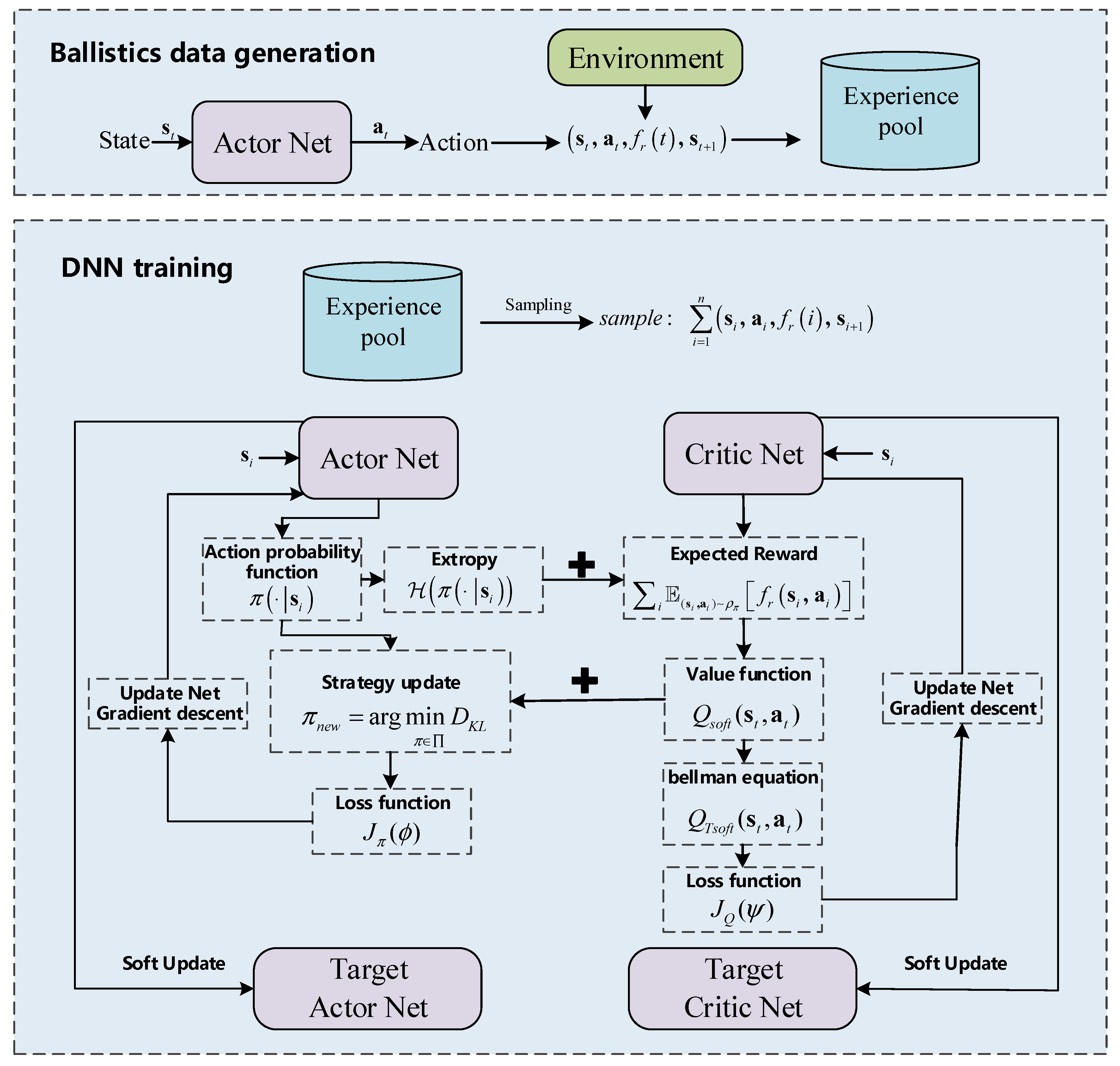
The frame of sac networks is shown in the Figure 5, consists of Actor net and Critic net. Actor net is generating action, and environment returns the reward and next state. All of ballistics data is stored in experience pool, including state, action, reward, and next state.
Critic net is used to judge the found strategies, which guides impartially the strategy of Actor network. At the beginning, Actor net and Critic net are given random parameters. Actor net is difficult generating the optimal strategy, and Critic net is difficult judging scientifically towards the strategy of Actor net. The parameters of networks are need to update based on continuously generating and sampling ballistics data.
For updating Critic net, Critic net outputs the expected reward based on samples, and Actor net outputs the action probability, which is depicted by entropy term . Combining with , the value function is conducted and shown in Eq.(47)
Further obtain the Bellman equation:
Given by Eq.(49), the loss function of Critic net is acquired:
For updating Actor net, the updating strategy is shown in Eq.(50)
where, represents the set of strategy, is partition function, used to normalized distribution. is Kullback-Leibler (KL) divergence [25].
Combining re-parameterization technique with Eq.(51), the loss function of Actor net is obtained:
In which , is the input noise, obeying the distribution .
The method of stochastic gradient descent is introduced to minimize the loss function of networks. The optimal parameters of Actor-Critic networks are obtained with repeating the updating process, passing respectively the parameters to target networks via soft-updating.
Figure 5.
updating principle of SAC.
5.2. Meta SAC Optimization Algorithm
The learning algorithm in DRL relies on a lot of interaction between agent and environment, and high training costs. Once the environment changed, the original strategy is no longer applicable, and need to learn from scratch. The penetration guidance problem under the stable flight environment can be solved by SAC networks. For the changeable flight environment, such as the initial position of interceptor changes greatly, or the interceptor guidance law deviates greatly from preset value, the strategy solved by traditional SAC is hard to adapt, which is need to restudy and redesign. The manuscript introduces Meta learning to optimize and improve SAC performance. The training goal of Meta SAC is to obtain initial SAC model parameters. When the UAV penetration mission is changed, through a few scenes of learning, the UAV can adapt to new environment and complete the corresponding guidance penetration mission, without relearning model parameters. Meta SAC can achieve “learn while flying” for UAV, and strengthen the adaptability of UAV.
The Meta SAC algorithm is shown in Algorithm 1, which is divided into meta training and meta testing phase. Meta training phase is to solve the optimal meta learning parameters based on multi-experience missions. In the meta testing phase, the trained meta parameters are interactively learned with the new mission environment to fine-tune the meta parameters.
| Algorithm 1 Meta SAC |
| 1: Initialize the experience pool ,Storage space N 2: Meta training: 3: Inner loop 4: for iteration k do 5: sample mission(k) from 6: update actor policy to using SAC based on mission(k): 7: . 9: Outer loop 10: 11:Generate from Θ and estimate the reward of Θ. 12: Add a hidden layer feature as a random noise. 13: 14: The meta learning process of different missions is carried out through SGD. 15: for iteration mission(k) do 16: 17: 18: Meta testing 19: Initialize the experience pool ,Storage space N. 20: Load meta training network parameters . 21: Set training parameters. 22: for iteration i do 23: sample mission from 24: End for |
The basic assumption of Meta SAC is that the experience mission for meta training and the new mission for meta testing obey the same mission distribution . Therefore, there are some common characteristics between different missions. In the DRL scenario, our goal is to learn a function with parameter , which can minimize the loss function of specific mission . In the Meta DRL scenario, our goal is to learn a learning process , which can quickly adapt to the new mission with a very small dataset . Meta SAC can be summarized as optimizing the parameters , in the learning process:
where and respectively represent training and testing missions sampled from , represents the testing loss function. In the meta training phase, parameters are optimized by inner loop and outer loop.
In the inner loop, Meta SAC updates model parameters with a small amount of randomly selected data of specific mission as the training data, reducing the loss of model on mission . In this part, updating of model parameters is the same as the original SAC algorithm, and the agent learns several scenes on randomly selected missions.
The minimum mean square error of strategy parameters corresponding to different missions in the inner loop phase is solved to obtain the initial strategy parameters of the outer loop. In this manuscript, a hidden layer feature is added to the input part of strategy as a random noise. The random noise is sampled again in each episode, in order to provide a more continuous random exploration in time, which is helpful for agent to adjust their overall strategy exploration according to the current mission MDP. The goal of Meta learning is to let agent learn how to quickly adapt to new missions by simultaneously updating a small amount of gradient of strategy parameters and hidden layer features. Therefore, the of includes not only parameters of the neural network, but also the distribution parameters of hidden variables of each mission, namely the mean and variance of the Gaussian distribution, as shown in Eq.(53).
The model is represented by a parameterized function with parameter , and when it is transferred to a new mission , model parameter is updated to through gradient rise, as shown in Eq.(54).
Update step is a fixed super parameter. Model parameter is updated to maximize the performance of different missions, as shown in Eq.(55).
The meta learning process of different missions is carried out through SGD, and the principle of is:
where is meta update step.
In the meta testing phase, a small amount of experience in new missions is used to quickly learn strategies for solving new missions. A new mission may involve completing a new mission goal or achieving the same mission goal in a new environment. The updating process of model in this phase is the same as the cycle part in the meta training phase, by calculating the loss function with the data collected in the new mission, adjusting the model through back propagation, at last, new mission is adapted by agent.
6. Simulation Analysis
In this section, the manuscript analyzes and verifies escape guidance strategy based on Meta SAC. SAC is used to solve specific escape guidance mission. We conduct comprehensive experiments to verify whether the UAV can complete the guidance escape mission under satisfying terminal constraints and process constraints. Once the UAV guidance escape mission changes, the original strategy based on SAC is difficult to adapt to the changed mission, which is need to be relearned and retrained. The manuscript proposes an optimization method via Meta learning, which improves the learning ability of UAV during the training process. This section focuses on verifying the validation of Meta SAC, demonstrating the performance in various new missions. Besides, the maneuvering overload commands under different pursuit evading distances are analyzed, which is used to explore the influence of different maneuvering timings and distances on the escape results. Taking CAV-H to verify the escape guidance performance. The initial conditions, terminal altitude and Meta SAC training parameters are given in Table 1.
6.1. Validity verification on SAC
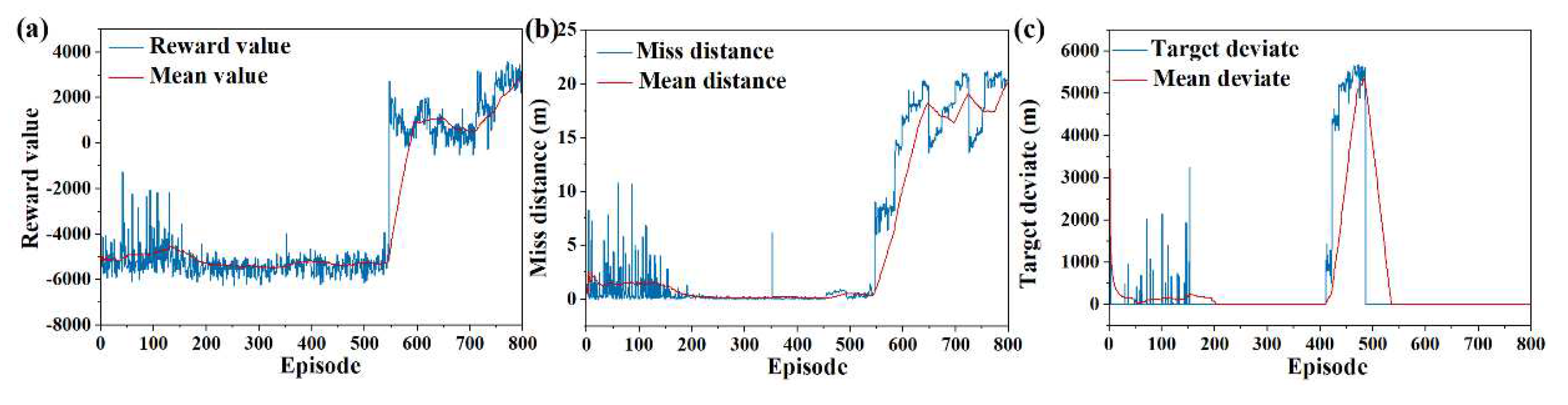
In order to verify the effectiveness of SAC, three different pursuit evading scenarios are constructed, and the terminal reward value, miss distance and terminal position deviate are respectively analyzed. As shown in Figure 8(a), the terminal reward value is poor in the initial phase of training, which manifests the optimal strategy is not found. After 500 episodes, the terminal reward value increases gradually, indicating better strategy is explored and converged. At the last 100 episodes, the optimal strategy is trained and learned, meanwhile, the network parameters have been adjusted to the optimal. As can be seen from Figure 8(b), the miss distance is relatively divergent in the first 150 episodes of training, indicating the action network in SAC is constantly exploring new strategies, and the critic network is also learning scientific evaluation criteria. After 500 training episodes, the network is gradually learning and training in the direction of optimal solution. The miss distance at the encounter moment converges to about 20m. As shown in Figure 8(c), the terminal position of UAV has a large deviation in the early training phase, which is attributed to the exploration of escape strategy by network. In the later training phase, the position deviation is less affected by exploration. These pursuit evading scenarios tested in the manuscript can achieve convergence, and the final convergence values are all within 1m.
Figure 6.
Train results of SAC. (a) reward value, (b) miss distance, (c) target deviate.
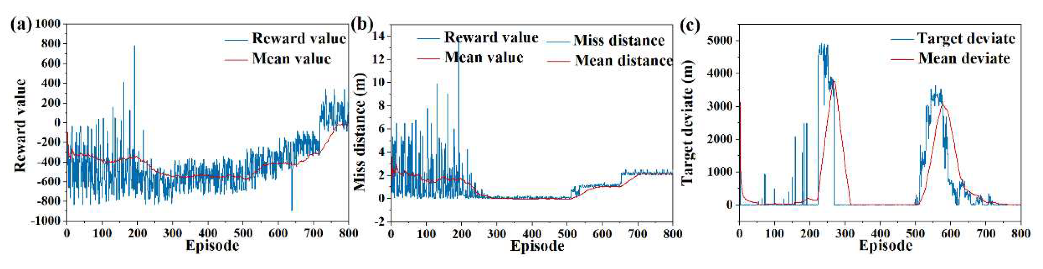
In order to verify whether the SAC algorithm can solve the escape guidance strategy that meets the mission requirements in different pursuit and evasion scenarios, the pursuing and evading distance is changed, and the training results are shown in the Figure 7. In medium range scenario, the miss distance converges to about 2m, and the terminal deviation converges to about 1m.
Figure 7.
Train results of SAC. (a) reward value, (b) miss distance, (c) target deviate.
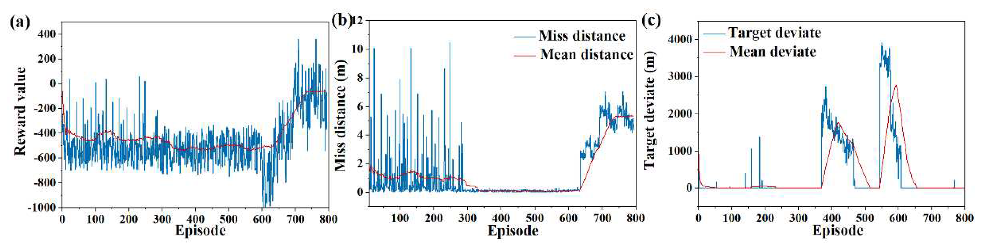
As shown in Figure 8, In long range attack and defense scenarios, the miss distance converges to about 5m, and the terminal deviation converges to about 1m.
Figure 8.
Train results of SAC. (a) reward value, (b) miss distance, (c) target deviate.
Based on above simulation analysis, SAC is a feasible method to solve the UAV guidance escape strategy. After limited episodes of learning and training, network parameters are converged, which is used to test on flight mission.
6.2. Validity Verification on Meta SAC
When the mission of UAV changes, the original SAC parameters can not meet acquirements of new mission,which needs to be re-trained and learned. The SAC proposed in the manuscript is improved via Meta learning. Strong adaptive network parameters are found by learning and training, when the pursuit evading environment changes, the network parameters is fine-tuned to adapt to the new environment immediately.
Meta SAC is divided into meta training phase and meta testing phase, Initialization parameters for SAC network are trained in meta training phase, which is fine-tuned by interacting with the new environment in meta testing phase. By changing the initial interceptor position, three different pursuit evading scenarios are constructed, which respectively represents short distance, medium and long distance.
Training results of Meta SAC and SAC are compared, terminal reward values are represented as shown in Figure 9(a). Meta SAC is an effective method to speed up the training process, after 100 episodes, better strategy is learned by the network and converged gradually, contraryly, the SAC network needs 500 episodes to find the optimal solution. Miss distance is shown in Figure 9(b). The better strategy is quickly learned by Meta SAC, which is more effective than the SAC method. Figure 9(c) show the terminal deviate between UAV and target.
To explore the optimal solution as much as possible, some strategies with large terminal position deviation appear in the training process. As shown in Figure 10(b-c), in medium range attack and defense scenarios, the miss distance converges to about 8m based on Meta SAC, and the terminal deviation converges to about 1m.
As shown in Figure 11(b-c), in long range attack and defense scenarios, the miss distance converges to about 10m based on Meta SAC, and the terminal deviation converges to about 1m.
According to the theoretical analysis, in the training process, new missions corresponding to the same distribution are used to execute micro-testing by Meta SAC, resulting in more gradient descending directions of optimal solution are learned by network. Combined with the theory analysis and training results, the manuscript manifests Meta learning is a feasible method to accelerate convergence and improve the efficiency of training.
In the previous analysis, when the pursuit evading secenerio is changed, network parameters obtained in the meta training phase are fine-tuned through few interactions. The manuscript verifies meta testing performance by changing the initial interceptor position, and results compared with SAC method are shown in the Table 2. Based on the network parameters of meta training phase, the strategic solutions meeting escape guidance missions are found through training within 10 episodes. On the contrary, network parameters based on SAC need more interaction to find solutions, and the the episode of interactions is basically more than 50 episodes. According to above simulation, the adaptability of Meta SAC is much greater than SAC, once the escape mission changing, through very few episodes of learning, the new mission is completed by UAV without re-learning and designing strategy. The method provides possibility for realizing UAV learning while flying.
6.3. Strategy Analysis Based on Meta SAC
This section tests the network parameters based on Meta SAC, and analyzes the escape strategy and flight state under different pursuit evading distances. As shown in Figure 12(a), for the pursuit evading scene of short distance, the longitudinal maneuvering overload is larger in the first half phase of escape, resulting in velocity slope angle decreases gradually. In the second half phase of escape, if strategy is executed under the original maneuvering overload, the terminal altitude constraint can not be satisfied, therefore, the overload gradually decreases, the velocity slope angle is slowly reduced. As shown from Figure 12(b), at the beginning of escape, the lateral maneuvering overload is positive, and the velocity azimuth angle is constantly increasing. With the distance between UAV and interceptor reducing, the overload increases gradually in the opposite direction, and the velocity azimuth angle decrease. On the one hand, it can confuse the strategy of interceptor, on the other hand, the guidance course is corrected.
As shown in Figure 13(a), compared with the pursuit evading scene of short distance, the medium escape process takes longer, the pursuing time left to interceptor is longer, and the UAV flies under the direction of increasing the velocity slope angle. The timing of maximum escape overload corresponding to the medium distance is also different. As shown in Figure 13(b), in the first half phase of escape, lateral maneuvering overload corresponding to medimum distance is larger than that in the short distance, and in the second half phase of the escape, the corresponding reverse maneuvering overload is smaller, resulting in UAV can use the longer escape time to slowly correct the course.
As shown in Figure 14, under the long pursuit distance, the overload change of UAV maneuver is similar to that of medium range, and the escape timing is basically the same as the escape strategy.
According to the above analysis, the escape guidance strategy via Meta SAC can be used as a tactical escape strategy, and the timing of escape and maneuvering overload are adjusted timely under different pursuit evading distances. On the one hand, the overload corresponding to this strategy can confuse the interceptor and cause some interference, on the other hand, it can take into account the guidance mission, correcting the course deviation caused by escape.
Figure 15(a) shows the flight trajectory of interceptor against UAV at the North East Down (NED) coordinate (10 km,30 km,30 km), the trajectory point at the encountering moment is shown in Figure 15(b), and the miss distance is 19 m in this pursuit evading scene. To verify the scientific and applicability of Meta SAC, the initial position of interceptor is changed. Flight trajectories are respectively represented shown in Figure 15(c,e), and trajectory points at the encountering moment are shown in Figure 15(d,f). The miss distances in these two pursuit evading scenarios are 3 m and 6 m respectively. Based on the CAV-H structure, the miss distance between UAV and interceptor is greater than 2 m at the encountering moment, which means the escape mission is achieved.
Based on the principle of Meta SAC and optimal guidance, flight states are shown in the Figure 16. Longitude, latitude and altitude during flight of UAV are shown in Figure 16(a)-(b), under different pursuit evading scenarios, terminal position and altitude constraints are meet. There is larger amplitude modification in the velocity slope and azimuth angle, which is attributed to escape strategy via lateral and longitudinal maneuvering, as shown in Figure 16(c)-(d). The total change of velocity slope and azimuth angle is within two degrees, which meets flight process constraints. Through the analysis of flight states, this escape strategy is an effective measure for guidance escape with high accuracy.
Flight process deviation mainly includes aerodynamic calculation deviation and output overload deviation. For the aerodynamic deviation, the manuscript uses interpolation method to calculate based on the flight Mach number and angle of attack, which may have some deviation. Therefore, when calculating the aerodynamic coefficient, random noise with an amplitude of 0.1 is added to verify whether the UAV can complete the guidance mission. As shown in Figure 17 (a), aerodynamic deviation noise causes certain disturbances to the angle of attack during flight. At the 10th second and end of flight, the maximum deviation of the angle of attack is 2 °. However, overall, the impact of aerodynamic deviation on the entire flight is relatively small, and the change in angle of attack is still within the safe range of the UAV. As shown in Figure 17 (b), due to the constraints of UAV game confrontation and guidance missions, the bank angle during the entire flight process changes significantly, and aerodynamic deviation noise has a small impact on the bank angle. After increasing the aerodynamic deviation noise, the miss distance between the UAV and the interceptor at the time of encounter is 8.908m, and the terminal position deviation is 0.52m. Therefore, under the influence of aerodynamic deviation, the UAV can still complete the escape guidance mission.
For the output overload deviation, the total overload is composed of the guiding overload derived from the optimal guidance law and the maneuvering overload output from the neural network. random maneuvering overload with an amplitude of 0.1 is added to verify whether the UAV can complete the maneuver guidance mission. As shown in Figure 18, random overloads are added in the longitudinal and lateral directions respectively. Through simulation testing, the miss distance between the UAV and the interceptor at the encounter point is 10.51m, and the terminal deviation of the UAV is 0.6m. Under this deviation, the UAV can still achieve high-precision guidance and efficient penetration.
7. Conclusion
The manuscript proposes escape guidance strategy satisfying terminal multiple constraints via SAC. The action space is designed under the UAV process constraint. Considering the fact that the real-time interceptor information is hard to obtain in the actual escape process, the state space considering the target and the heading angle is designed. The reward function is an important index function, which is used to guide and evaluate the training results. Based on the pursuit evading model, terminal LOS angle rates of lateral and longitudinal are derived to describe the deviation and miss distance. In order to improve the adaptability of escape guidance strategy, the manuscript improves SAC via meta learning, and compares meta SAC with SAC. The strong adaptive escape strategy based on meta SAC is analyzed. In view of the above theoretical numerical analysis, we have obtained the following conclusions.
- (1)
- The escape guidance strategy based on SAC is a feasible tactical escape strategy, which can achieve high precision guidance under meeting the escape requirements.
- (2)
- Meta SAC can significantly improve the adaptability of escape strategy. When the escape mission changes, it can fine-tune network parameters to adapt to mission through a small number of training. This method provides a possibility for the UAV to learn while flying.
- (3)
- The strong adaptive escape strategy based on meta SAC can adjust the escape timing and maneuvering overload in real time according to the pursuit evading distance. On the one hand, the overload corresponding to this strategy can confuse the interceptor and cause some interference, on the other hand, it can take into account the guidance mission, correcting the course deviation caused by escape.
Author Contributions
Conceptualization, SiBo Zhao. and JianWen Zhu.; methodology, SiBo Zhao.; software, SiBo Zhao; validation, SiBo Zhao. and JianWen. Zhu; formal analysis, SiBo Zhao; investigation, SiBo Zhao.; resources, XiaoPing Li.; data curation, HaiFeng Sun.; writing—original draft preparation, HaiFeng Sun.; writing—review and editing, XiaoPing Li.; visualization, SiBo Zhao.; supervision, WeiMin Bao. All authors have read and agreed to the published version of the manuscript.
Funding
This research received no external funding.
Data Availability Statement
Not applicable.
Conflicts of Interest
The authors declare no conflict of interest.
References
- H. W. LI ZB, Z. J. S. ZHANG, and T. n. Review, "Summary of the Hot Spots of Near Space Vehicles in 2018," vol. 37, no. 1, p. 44, 2019. [CrossRef]
- Li, G.; Zhang, H.; Tang, G. Maneuver characteristics analysis for hypersonic glide vehicles. Aerosp. Sci. Technol. 2015, 43, 321–328. [CrossRef]
- Wang, L.; Lan, Y.; Zhang, Y.; Zhang, H.; Tahir, M.N.; Ou, S.; Liu, X.; Chen, P. Applications and Prospects of Agricultural Unmanned Aerial Vehicle Obstacle Avoidance Technology in China. Sensors 2019, 19, 642. [CrossRef]
- Y. WANG, T. ZHOU, W. CHEN, T. J. J. o. B. U. o. A. HE, and Astronautics, "Optimal maneuver penetration strategy based on power series solution of miss distance," vol. 46, no. 1, p. 159. [CrossRef]
- Rim, J.-W.; Koh, I.-S. Survivability Simulation of Airborne Platform With Expendable Active Decoy Countering RF Missile. IEEE Trans. Aerosp. Electron. Syst. 2019, 56, 196–207. [CrossRef]
- Liu, F.; Dong, X.; Li, Q.; Ren, Z. Robust multi-agent differential games with application to cooperative guidance. Aerosp. Sci. Technol. 2021, 111, 106568. [CrossRef]
- E. Garcia, D. W. Casbeer, and M. J. I. T. o. A. C. Pachter, "Design and analysis of state-feedback optimal strategies for the differential game of active defense," vol. 64, no. 2, pp. 553-568, 2018. [CrossRef]
- H. Liang, W. Jianying, W. Yonghai, W. Linlin, and L. J. C. J. o. A. Peng, "Optimal guidance against active defense ballistic missiles via differential game strategies," vol. 33, no. 3, pp. 978-989, 2020. [CrossRef]
- Liang, L.; Deng, F.; Peng, Z.; Li, X.; Zha, W. A differential game for cooperative target defense. Automatica 2019, 102, 58–71. [CrossRef]
- Liu, S.; Wang, Y.; Li, Y.; Yan, B.; Zhang, T. Cooperative guidance for active defence based on line-of-sight constraint under a low-speed ratio. Aeronaut. J. 2022, 127, 491–509. [CrossRef]
- D. Zhang, T. Zhang, Y. Lu, Z. Zhu, and B. J. A. i. N. I. P. S. Dong, "You only propagate once: Accelerating adversarial training via maximal principle," vol. 32, 2019.
- Ruthotto, L.; Osher, S.J.; Li, W.; Nurbekyan, L.; Fung, S.W. A machine learning framework for solving high-dimensional mean field game and mean field control problems. Proc. Natl. Acad. Sci. 2020, 117, 9183–9193. [CrossRef]
- Ullah, Z.; Al-Turjman, F.; Mostarda, L.; Gagliardi, R. Applications of Artificial Intelligence and Machine learning in smart cities. Comput. Commun. 2020, 154, 313–323. [CrossRef]
- Song, H.; Bai, J.; Yi, Y.; Wu, J.; Liu, L. Artificial Intelligence Enabled Internet of Things: Network Architecture and Spectrum Access. IEEE Comput. Intell. Mag. 2020, 15, 44–51. [CrossRef]
- Gong, X.; Chen, W.; Chen, Z. All-aspect attack guidance law for agile missiles based on deep reinforcement learning. Aerosp. Sci. Technol. 2022, 127. [CrossRef]
- Furfaro, R.; Scorsoglio, A.; Linares, R.; Massari, M. Adaptive generalized ZEM-ZEV feedback guidance for planetary landing via a deep reinforcement learning approach. Acta Astronaut. 2020, 171, 156–171. [CrossRef]
- Yuan, Y.; Zheng, G.; Wong, K.-K.; Letaief, K.B. Meta-Reinforcement Learning Based Resource Allocation for Dynamic V2X Communications. IEEE Trans. Veh. Technol. 2021, 70, 8964–8977. [CrossRef]
- Zhao, L.-B.; Xu, W.; Dong, C.; Zhu, G.-S.; Zhuang, L. Evasion guidance of re-entry vehicle satisfying no-fly zone constraints based on virtual goals. Sci. Sin. Phys. Mech. Astron. 2021, 51, 104706. [CrossRef]
- Guo, Y.; Li, X.; Zhang, H.; Wang, L.; Cai, M. Entry Guidance With Terminal Time Control Based on Quasi-Equilibrium Glide Condition. IEEE Trans. Aerosp. Electron. Syst. 2020, 56, 887–896. [CrossRef]
- Krasner, S.M.; Bruvold, K.; Call, J.A.; Fieseler, P.D.; Klesh, A.T.; Kobayashi, M.M.; Lay, N.E.; Lim, R.S.; Morabito, D.D.; Oudrhiri, K.; et al. Reconstruction of Entry, Descent, and Landing Communications for the InSight Mars Lander. J. Spacecr. Rocket. 2021, 58, 1569–1581. [CrossRef]
- Huang, Z.C.; Zhang, Y.S.; Liu, Y. Research on State Estimation of Hypersonic Glide Vehicle. J. Physics: Conf. Ser. 2018, 1060, 012088. [CrossRef]
- Zhu, J.; Su, D.; Xie, Y.; Sun, H. Impact time and angle control guidance independent of time-to-go prediction. Aerosp. Sci. Technol. 2019, 86, 818–825. [CrossRef]
- Ni, C.; Zhang, A.R.; Duan, Y.; Wang, M. Learning Good State and Action Representations via Tensor Decomposition. 2021, 1682–1687. [CrossRef]
- Ma, Y.; Wang, Z.; Castillo, I.; Rendall, R.; Bindlish, R.; Ashcraft, B.; Bentley, D.; Benton, M.G.; Romagnoli, J.A.; Chiang, L.H. Reinforcement Learning-Based Fed-Batch Optimization with Reaction Surrogate Model. 2021. [CrossRef]
- X. Yang et al., "Learning high-precision bounding box for rotated object detection via kullback-leibler divergence," vol. 34, pp. 18381-18394, 2021.
Figure 1.
Attack-defense model.
Figure 2.
guidance penetration strategy.
Figure 3.
The attack defense confrontation model in lateral direction.
Figure 4.
The attack defense confrontation model in longitudinal direction.
Figure 9.
Meta SAC training results. (a) Reward value, (b) miss distance, (c) target deviate.
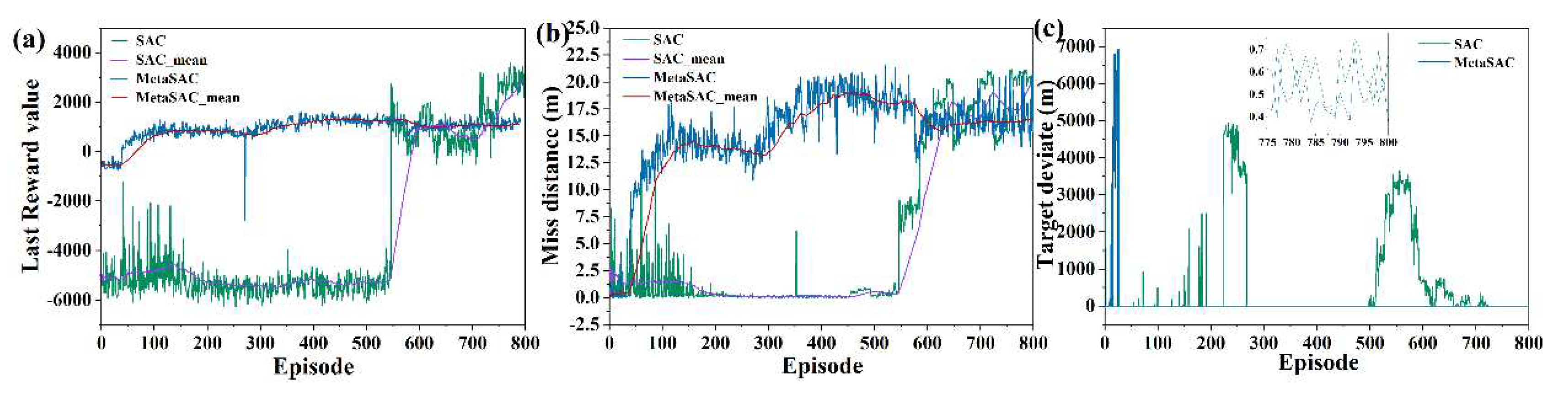
Figure 10.
Meta SAC training results. (a) Reward value, (b) miss distance, (c) target deviate.
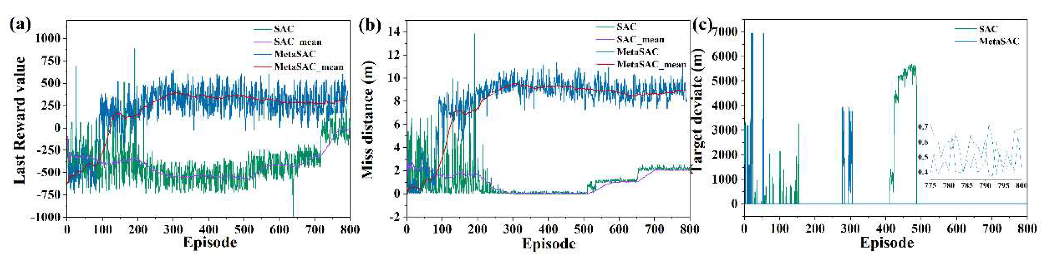
Figure 11.
Meta SAC training results. (a) Reward value, (b) miss distance, (c) target deviate.
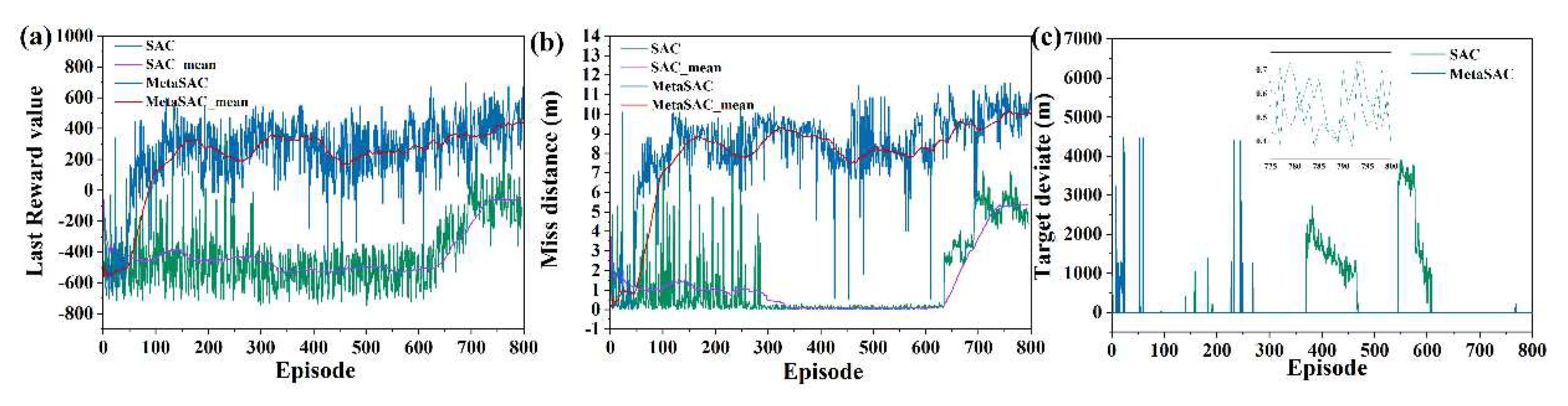
Figure 12.
the maneuvering overload. (a) longitudinal direction under short distance, (b) lateral direction under short distance.
Figure 12.
the maneuvering overload. (a) longitudinal direction under short distance, (b) lateral direction under short distance.
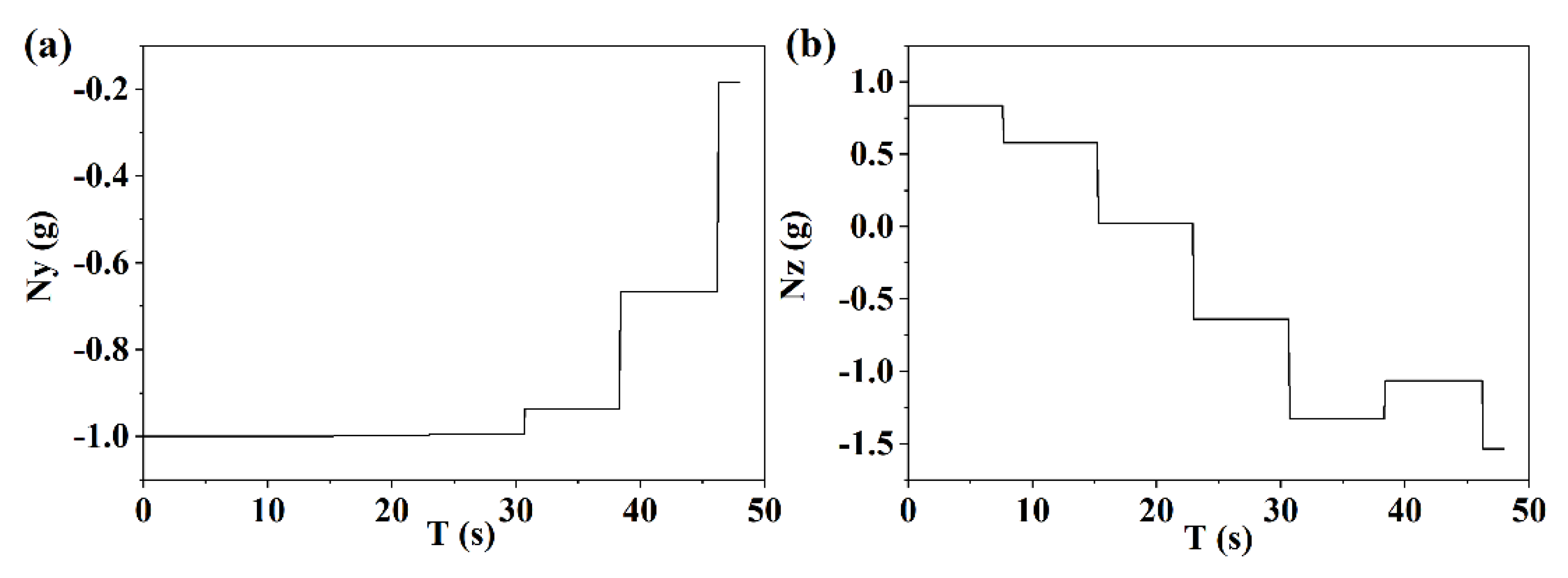
Figure 13.
the maneuvering overload. (a) longitudinal direction under medimum distance, (b) lateral direction under medium distance.
Figure 13.
the maneuvering overload. (a) longitudinal direction under medimum distance, (b) lateral direction under medium distance.
Figure 14.
the maneuvering overload. (a) longitudinal direction under long distance, (b) lateral direction under long distance.
Figure 14.
the maneuvering overload. (a) longitudinal direction under long distance, (b) lateral direction under long distance.
Figure 15.
The ballistic flight diagrams of whole course under different pursuit evading distances, (b) and (d) and (f) represent trajectories at the encountering time under different pursuit evading distances.
Figure 15.
The ballistic flight diagrams of whole course under different pursuit evading distances, (b) and (d) and (f) represent trajectories at the encountering time under different pursuit evading distances.
Figure 16.
Flight states of UAV. (a) the longitude and latitude, (b) the height, (c) the velocity slope angle, (d) the velocity azimuth angle.
Figure 16.
Flight states of UAV. (a) the longitude and latitude, (b) the height, (c) the velocity slope angle, (d) the velocity azimuth angle.
Figure 17.
a) the attack angle, (b) the bank angle.
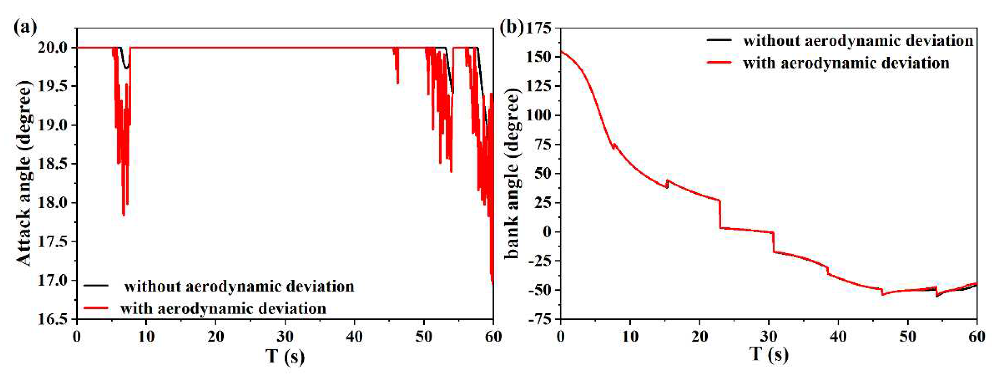
Figure 18.
(a) the maneuvering overload in the longitudinal direction, (b) the maneuvering overload in the lateral direction.
Figure 18.
(a) the maneuvering overload in the longitudinal direction, (b) the maneuvering overload in the lateral direction.
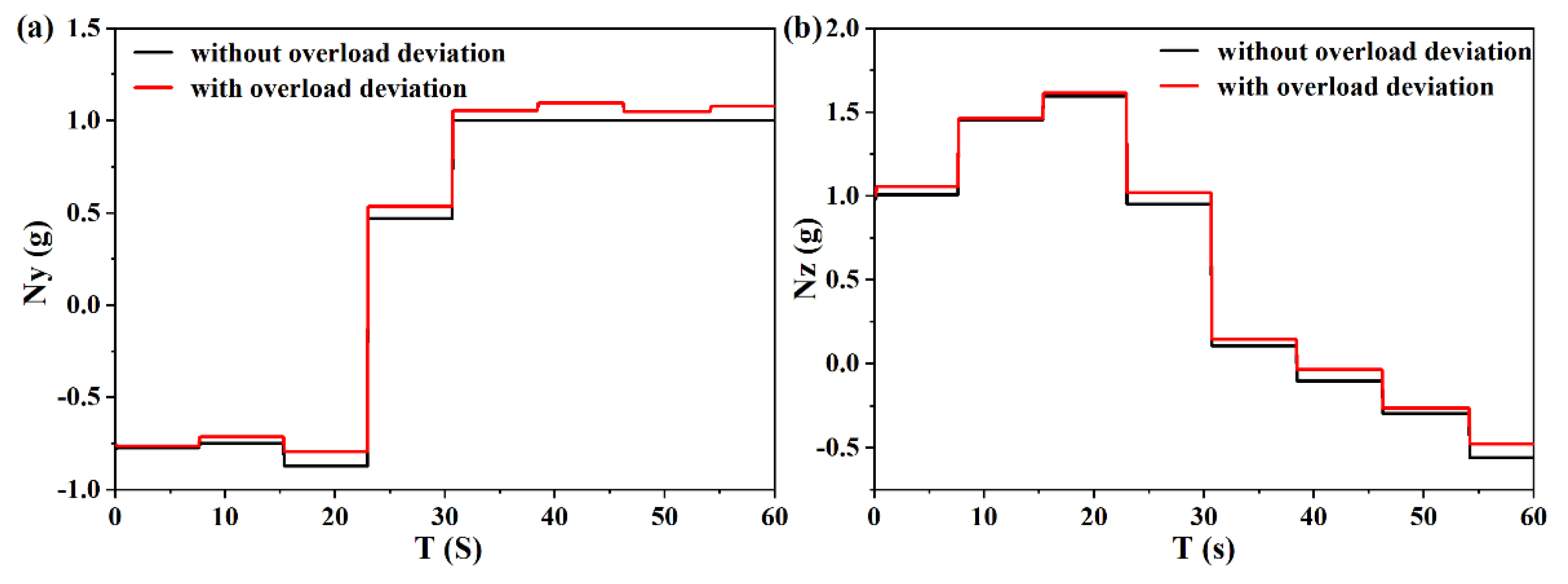

Table 1.
Simulation and Meta SAC training conditions.
| Simulation Conditions | Meta SAC Training Parameters | ||
|---|---|---|---|
| UAV initial velocity | 4000m/s | Learning episodes | 1000 |
| Initial velocity Inclination | 0° | Guidance period | 0.1s |
| Initial velocity azimuth | 0° | Data sampling interval | 30Km |
| Initial position | (3°E, 1°N) | Discount factor | = 0.99 |
| Initial altitude | 45km | Soft update tau | 0.001 |
| Terminal altitude | 40km | Learing rate | 0.005 |
| Target position | (0°E, 0°N) | Sampling size for each train | 128 |
| Interceptor Initial velocity | 1500m/s | Net layers | 2 |
| Initial velocity Inclination | longitudinal LOS angle | Net nodes | 256 |
| Initial velocity azimuth | lateral LOS angle | Capacity of experience pool | 20000 |
Table 2.
Results compared with SAC method.
| Interceptor Initial position (Km) |
Interaction episodes | Miss distance (m) | Terminal deviate (m) | |||
|---|---|---|---|---|---|---|
| SAC | Meta SAC | SAC | Meta SAC | SAC | Meta SAC | |
| (0, 30, 0) | 74 | 1 | 3.78 | 3.29 | 0.56 | 0.61 |
| (2, 30, 6) | 75 | 4 | 2.80 | 2.72 | 0.68 | 0.72 |
| (4, 30, 12) | 59 | 8 | 6.93 | 3.75 | 0.69 | 0.58 |
| (6, 30, 18) | 59 | 1 | 2.71 | 6.82 | 0.68 | 0.72 |
| (8, 30, 24) | 26 | 2 | 3.16 | 3.70 | 0.47 | 0.50 |
| (10, 30, 30) | 58 | 3 | 3.50 | 2.37 | 0.61 | 0.64 |
| (12, 30, 36) | 67 | 1 | 2.86 | 2.21 | 0.68 | 0.45 |
| (14, 30, 42) | 56 | 8 | 2.18 | 2.89 | 0.55 | 0.61 |
| (16, 30, 48) | 69 | 1 | 2.73 | 2.23 | 0.61 | 0.72 |
| (18, 30, 54) | 106 | 1 | 2.45 | 3.71 | 0.56 | 0.63 |
| (20, 30, 60) | 94 | 1 | 2.7 | 2.35 | 0.49 | 0.54 |
| (22, 30, 66) | 59 | 1 | 2.23 | 2.51 | 0.73 | 0.71 |
| (24, 30, 72) | 62 | 1 | 2.11 | 3.47 | 0.48 | 0.67 |
| (26, 30, 78) | 63 | 1 | 2.04 | 4.5 | 0.48 | 0.57 |
| (28, 30, 84) | 63 | 4 | 2.64 | 5.12 | 0.47 | 0.40 |
| (30, 30, 90) | 63 | 9 | 2.95 | 6.05 | 0.68 | 0.47 |
Disclaimer/Publisher’s Note: The statements, opinions and data contained in all publications are solely those of the individual author(s) and contributor(s) and not of MDPI and/or the editor(s). MDPI and/or the editor(s) disclaim responsibility for any injury to people or property resulting from any ideas, methods, instructions or products referred to in the content. |
© 2023 by the authors. Licensee MDPI, Basel, Switzerland. This article is an open access article distributed under the terms and conditions of the Creative Commons Attribution (CC BY) license (http://creativecommons.org/licenses/by/4.0/).
Copyright: This open access article is published under a Creative Commons CC BY 4.0 license, which permit the free download, distribution, and reuse, provided that the author and preprint are cited in any reuse.


