
Submitted:
17 August 2023
Posted:
18 August 2023
You are already at the latest version
Abstract
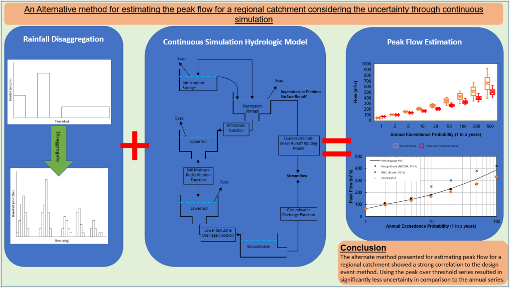
Estimating peak flow for a catchment is commonly undertaken using the design event method, however this method does not allow for the understanding of uncertainty in the result. This research first presents a simplified method of fragments approach to rainfall disaggregation that ignores the need to consider seasonality, offering a greater diversity in storm patterns within the resulting sub-daily rainfall. By simulating 20 iterations of the disaggregated sub-daily rainfall within a calibrated continuous simulation hydrologic model, we were able to produce multiple long series of stream flow at the outlet of the catchment. With this data, we investigated the use of both the annual maximum and peaks over threshold approaches to flood frequency analysis and found that for a one in 100 year annual exceedance probability peak flow, the peaks over threshold method (333m3/s ±50m3/s) was significantly less uncertain than the annual maximum method (427m3/s ±100m3/s). For the one in 100 year annual exceedance probability, the median peak flow from the peaks over threshold method (333m3/s) produced an outcome comparable to the design event method peak flow (328m3/s), indicating that this research offers an alternative approach to estimating peak flow, with the additional benefit of understanding the uncertainty in the estimation. Finally, the paper highlighted the impact that length and period of streamflow has on peak flow estimation and noted that previous assumptions around the minimum length of gauged streamflow required for flood frequency analysis may not be appropriate in particular catchments.
Keywords:
Uncertainty
; Flood Frequency
; Rainfall Disaggregation
; Peak Flow Continuous Simulation
1. Introduction
Estimating peak flow rates from a catchment has long been a focus of engineering hydrologists and is fundamental to the design of flood protection infrastructure [1]. Understanding the uncertainty associated with peak flow estimation is however often neglected by practitioners, despite the acceptance that many sources of uncertainty exist [2]. The commonly used design event method, which adopts a probability neutral conversion of rainfall to runoff, fails to consider the impact that antecedent moisture conditions have in the derivation of hydrologic losses. [3] detailed the benefits of continuous simulation over the design event method with their development of a calibrated hydrologic model in a regional town in the state of Queensland, Australia. This paper expands on the research undertaken by the authors [3], whose focus was the calibration of the continuous simulation hydrologic model to historical events, with the aim of deriving flood frequency estimates with a greater understanding of uncertainty.
To estimate peak flows from a continuous simulation model, the data should normally follow a flood frequency distribution similar to gauged stream flow records. A model that can replicate a long series of stream flow (ie. continuous simulation) can assist in overcoming the shortcomings of stream gauge data, most noticeably the impact of urbanisation [1]. A flood frequency analysis (FFA) can be undertaken using one of two sampling approaches: annual maximum series and peaks over threshold (also known as partial series) [4]. The annual maximum series, while easier to identify independent flood events, produces less data points than the peaks over threshold series [5] but also prioritises the maximum annual flood over multiple larger floods that may have occurred in the same year. In contrast, the peaks over threshold offers added complexity due to the requirement to select an appropriate threshold flow. Some researchers found the best results of their FFA occurred when the number of data points (m) equaled the years of data (n) [6] [7], while others recommended a ratio of 1m:3n [8]. Both sampling approaches rely on a long series of continuous stream flow, with at least 50 years of data recommended to be used [9].
To produce a long series of continuous stream flow, a continuous simulation model requires an extended period of recorded rainfall at a suitable time step for the size and level of urbanisation of the catchment. In the case of a relatively small urban catchment, rainfall at a sub-hourly interval is required. Obtaining a recorded rainfall series of sufficient length over this time scale is extremely challenging given the lack of sub-daily rainfall gauges available in sparsely populated countries such as Australia, as illustrated in Figure 1. This contrasts recent reviews of global precipitation data, with some locations offering sub-daily rainfall that spans multiple decades [10]. The availability of sub-daily rainfall data has supported recent advancements in the use of continuous simulation hydrologic modelling [11], however, this research is unique in that the lack of availability of site based sub-daily rainfall data requires alternate considerations. To address this issue, sub-hourly rainfall can be generated from coarser timescale (daily) rainfall records through disaggregation [12] if historical daily rainfall data for at least 100 years is available for the site [13].
Many disaggregation approaches have been proposed in the literature and the most commonly used methods summarised in others [12], including parametric sampling methods such as the Poisson-cluster models and the random scale models, as well as nonparametric sampling methods like the Method of Fragments (MoF). They concluded that the MoF, first proposed as a method to disaggregate streamflow [14], was more flexible for operational use. At its core, the MoF simply disaggregates daily rainfall by selecting the pattern or ‘fragments’ of a known sub-daily event. The process of selection of suitable sub-daily events varies across the literature, including the use of the previous and subsequent day wetness to limit the sample size [15], or adding classes based on rainfall magnitude to ensure the daily rainfall was disaggregated based on sub-daily rainfall of a similar magnitude, as well as limiting the selection to events that occurred in the same month as the disaggregated rainfall [12]. While a long series of sub-daily rainfall data was produced, neither study used their dataset for continuous hydrologic modelling to estimate flood frequency.
This research offers new insight through the presentation of an alternate method for estimating peak flow in a small regional urban catchment. Through the inclusion of associated uncertainty, this method also offers a practical insight into how accurate regional authorities should consider their hydrological assessments to be. The results of this research also contribute significantly to the understanding of hydrologic uncertainty, especially in an urban catchment, where the reliance on accurate hydrologic modeling is at its’ greatest. By assessing the impact that the length and period of streamflow series has on peak flow estimation, we highlight the limitations associated with peak flow estimations from gauged catchments.
In particular, this research aims to develop a long series of sub-daily (6min) rainfall data for use in a continuous simulation model using a simplified version of the MoF and a long series of continuous flow data using the calibrated hydrologic model developed by the authors [3]. It will also estimate, with uncertainty, the peak flow for a range of annual exceedance probabilities and compare the results of this research to other methods. The materials and methods used in this research are described in Section 2 while Section 3 presents and discusses the results. Finally, our conclusions are presented in Section 4.
2. Materials and Methods
2.1. Continuous Simulation Model
A continuous simulation model was used in this research to estimate the peak flow for different annual exceedance probabilities. The model was developed by [3] for the Gowrie Creek catchment, a heavily urbanised 50 km2 catchment in the regional city of Toowoomba, in the state of Queensland, Australia. Toowoomba is considered to be sub-tropical with an average annual rainfall of 700 mm, the majority of which falls over the wet season from November to March. The extent of the catchment and its location in Australia, are shown in Figure 2.
While models for the catchment were calibrated to the historic rainfall and streamflow records, this research required additional steps to enable the continuous simulation model to be developed. Initially, daily rainfall data within the catchment for a 100 year period was obtained to allow the sub-daily rainfall disaggregation to be undertaken. This 100 year series of sub-daily rainfall data could then be simulated in a continuous simulation model to produce a 100 year time series of simulated streamflow. A FFA of this simulated streamflow was then undertaken to estimate peak flows of varying flood frequencies. This approach was repeated for 20 sub-daily rainfall disaggregation scenarios to facilitate the estimation of uncertainty in the results.
2.2. Daily Rainfall Data
Historical daily rainfall at the centroid of the catchment was sourced from SILO, a Queensland Government database containing continuous daily climate data for Australia from 1889 to the present day [13]. The 100 years of daily rainfall (year 1920 to 2020) used in this research is shown in Figure 3.
2.3. Sub-daily Rainfall Data
A long, continuous series of historical sub-daily rainfall data with a timestep shorter than the intended disaggregated timestep is needed to disaggregate the daily rainfall using the MoF. Historical sub-daily rainfall data is, however, limited in Australia as illustrated in Figure 1. To extend the sub-daily rainfall data duration and allow a wider variety of storm temporal patterns to be used, shorter durations of data from multiple gauging stations surrounding the catchment were sourced and ‘stacked’ to create a single longer series. This approach was used by [12] and found to achieve similar results to adopting a single sub-daily rainfall dataset. For the Gowrie Creek catchment specifically, only 12 years of sub-daily rainfall data was available, therefore data from rain gauges located outside the catchment was sourced. The location of the catchment and proximity and duration of the historical sub-daily rainfall was sourced from the Bureau of Meteorology and used in the rainfall disaggregation as shown previously in Figure 2.
2.4. Daily Rainfall Disaggregation
2.4.1. Method of Fragments
The MoF approach used [12]six major steps to disaggregate historical daily rainfall based on sub-daily rainfall data from multiple representative rainfall stations [12]. A key difference in this research was the exclusion of the need to only disaggregate daily rainfall using sub-daily storms that occur at a similar time of year or have similar rainfall on the day before or after the target day. The reasons for this are discussed further in Section 2.4.4.
The key steps adopted in this research to disaggregate historic daily rainfall to sub-daily rainfall were:
- Assign a storm class to both the historic daily and sub-daily rainfall series.
- Assign a unique storm number to each historic sub-daily storm.
- For a given day ‘x’ in the daily rainfall series, select a sub-daily storm with the same Storm Class.
- Disaggregate the daily rainfall based on the pattern of the sub-daily storm.
- Repeat Steps 3 and 4, ensuring the sub-daily storms are chosen uniformly to create an ensemble of disaggregated rainfall.
- Repeat all steps multiple times to create multiple iterations of disaggregated rainfall to understand the uncertainty.
2.4.2. Storm Class
An important consideration when using the MoF is the storm class. The storm class defines how the daily and sub-daily rainfall data sets are related as the daily rainfall data is only disaggregated to storms within the same storm class. It was initially suggested that only four storm classes be selected based on the rainfall before and after the day of interest [15]. However, this has a number of imitations including the potential for not considering important storms based on their insignificant pre/post day rainfall total. In addition, large daily rainfall totals could be disaggregated to high intensity, short duration and low depth storms based on the same pre/post rainfall conditions, rather than basing them on the magnitude of rainfall on the day of interest. The latter issue is of particular interest if the disaggregated rainfall is to be used in a hydrological model.
As a result, dividing the rainfall data into a number of storm classes was subsequently suggested, with an interval of 5mm being adopted [12]. This method was initially utilised in this research, however there were too few storms available for less frequent/more extreme daily rainfall totals. It was evident that multiple storm class options had to be considered and evaluated to determine the best approach.
2.4.3. Determination of the Number of Storm Classes
To ensure that the MoF was producing sub-daily rainfall data suitable for the hydrologic assessment, the results from three storm class options, presented in Table 1, were validated against the intensity-frequency-duration (IFD) data for the catchment. The IFD data represent design storm rainfall depths developed by the Australian Bureau of Meteorology and are commonly used in design event modelling.
To directly evaluate the MoF results from the class options assessed, IFD data was developed from the generated sub-daily rainfall. The annual maximum series was first modelled to the Generalised Extreme Value (GEV) distribution, as per the Bureau of Meteorology methodology for generating IFD data from historical sub-daily rainfall data [16]. A direct comparison of the MoF generated design rainfall depths to the Bureau of Meteorology generated design rainfall depths for the same duration and annual exceedance probability for different storm class options is shown in Figure 4. From this comparison, it was clear that class option 2 produced the best fit due to its proximity to the 1 in 1 line and was subsequently used in this research. The results suggest when moderate (>25mm/day) to extreme (>75mm/day) rainfall depths are being reached, the size of the class should be increased to allow a greater range of storms to be selected. Providing a larger number of smaller classes (class option 1) resulted in fewer storms to choose from, thereby decreasing the representation of the moderate to extreme rainfall events, while a smaller number of larger classes (class option 3) resulted in moderate daily rainfall depths being associated with more extreme storm patterns.
2.4.4. Seasonality
To best represent the range of storms possible and to understand the impact various storm patterns have on the catchment response to rainfall, it is important that a larger quantity of storms are available for use in the disaggregation. When reviewing the sub-daily rainfall data used in this research, it was clear that as the rainfall amount increased, the number of storms decreased significantly as shown in Figure 5 for class option 2. Previous studies that used the MoF approach ([12], [17], [18]) constrained the storm selection by incorporating seasonality, whereby the range of storms available for disaggregation were limited to those within a preset window around the day of rainfall being disaggregated. These previous studies did not, however, use the disaggregated rainfall in a hydrology model nor did they compare the results to IFD data. If this was undertaken, they would likely have seen that the same storm patterns would have been chosen multiple times to disaggregate the more extreme daily rainfall totals, and therefore produced similar peak flows, volumes and timing for multiple events, likely skewing any flood frequency analysis undertaken. To overcome this issue, this research has excluded seasonality as a constraint on storm selection, and instead adopted an approach whereby multiple iterations of disaggregated rainfall were simulated to better understand the uncertainty associated with the storm selection.
2.5. Hydrologic Model Simulation
The calibrated continuous simulation hydrologic model developed by the authors [3] was used in this research. A summary of the model development and calibration is provided below.
The hydrologic model of the Gowrie Creek catchment was developed using the modelling software XPRafts. The overall Gowrie Creek catchment was delineated into 23 sub-catchments, with each sub-catchment having a unique impervious fraction determined via regression analysis. The model was calibrated using the two-stage calibration approach [19,20]. The model offered a satisfactory fit (Nash Sutcliffe Efficiency > 0.5) for 9 of the 11 selected storm events, with seven events exceeding a Nash Sutcliffe Efficiency of 0.75. Events used in the calibration/validation included peak flows as low as 9 m3/s and as high as 600 m3/s.
The calibrated hydrologic model was simulated for a period of 100 years (1920 to 2020) of disaggregated historical daily rainfall. Twenty iterations of the disaggregated rainfall were simulated to allow the uncertainty in the results to be determined. While the model run times made running additional iterations prohibitive, increasing the number of iterations would have minimal impact on the outcomes of the research due to the small number of unique iterations possible, in particular for larger daily rainfall totals (as presented in Figure 5). This issue is further explored in Section 3.3.
2.6. Determination of Threshold Value
To allow the peaks over threshold flood frequency analysis of the long series of flow rates determined via continuous simulation, a threshold value is required. The data series used to undertake the flood frequency analysis is the maximum monthly flows above the threshold value. A higher threshold value will result in fewer values in the data series, while a lower threshold value will result in the opposite. In this research, we proposed an alternate method where we graphically interrogated the peak monthly flow from the full 100 years of continuous flow ranked in ascending order to determine clear changes in trend. Figure 6 shows three clear changes in trend at 45 m3/s, 70 m3/s and 110 m3/s.
Adopting the higher value of 110 m3/s resulted in a 0.5m:1n ratio which was considered a data series too small for a flood frequency analysis [6]. Adopting the lower value of 45 m3/s resulted in 3.2m:1n ratio, significantly higher than those documented in the literature. In addition, the trend change noted at 45 m3/s was not as clear as the other two changes in slope. Adopting the middle value of 70 m3/s resulted in a 1.2m:1n ratio which is in line with those documented in literature and graphically represents a clear change in trend, suggesting the flows below 70 m3/s would have a very frequent recurrence interval.
3. Results
3.1. Flood Frequency Analysis
A flood frequency analysis of all 20 iterations of the continuous simulation model was undertaken on the peaks over threshold series using a Bayesian fit of the Log Pearson Type 3 (LPIII) distribution [1]. The same flood frequency analysis was also undertaken using the available stream gauge data, with the combined results shown in Figure 7. As shown, all 20 simulations are within a relatively tight band. Given that all results are equally likely, we considered that the median would approximate the peak flow for a given AEP, with the range of possible results (or uncertainty bounds) being within the highest and lowest results of the simulation. This suggests that the 1 in 10-year AEP peak flow would be 166 m3/s ±20m3/s, while the 1 in 100-year AEP peak flow would be 333m3/s ±50m3/s.
In addition to the main finding above, the performance of the simulated results is also supported by the proximity of the same flood frequency analysis undertaken on the stream gauge. While the stream gauge result is at the upper end of the range of simulated results, it is posited that the shorter length of available stream gauge data (52 years), in comparison to the model simulations (100 years), is potentially skewing the stream gauge results. If the flood frequency analysis of the simulated results was undertaken for the same period and length of available stream gauge data (refer Figure 8), the simulated results better reflect the stream gauge data. What is also evident however is that the range of possible solutions increases significantly. Using the same approach as above, the 1 in 10 year AEP peak flow increases to 172m3/s ±30m3/s, while the 1 in 100 year AEP peak flow would increase to 360m3/s ±100m3/s. In practice it is recommended that at least 50 years of data is used in a flood frequency analysis [9]. This research indicates that data of this length may, however, be overestimating the result and increasing the uncertainty significantly.
While the length of available data is a well discussed criterion when undertaking a flood frequency analysis, the period of data adopted is often neglected. This issue is particularly evident in catchments like the Gowrie Creek catchment which may be considered to have a sufficient length of gauged data but recently experienced a flood event significantly larger than any others recorded. The impact of adopting the minimum of 50 years of stream flows over differing time periods (1920-1970, 1930-1980, 1940-1990, 1950-2000, 1960-2010 and 1970-2020) has been undertaken using one of the model simulations and is shown in Figure 9. These results show the impact that large floods (or the lack thereof) can have on the flood frequency analysis, with the 1 in 100-year AEP peak flow ranging from 308m3/s to 432m3/s.
3.2. Peaks Over Threshold vs Annual Maximum Series
As detailed in Section 1, the peaks over threshold method has been used in this research to develop the data series for flood frequency analysis. However, the annual maximum series is still used by most practitioners, and it was therefore worth highlighting the impact of adopting the alternative option. The results presented in Figure 10 show that the annual maximum series results in significantly higher peak flows for AEPs less frequent that a 1 in 5 year while also resulting in increased uncertainty in the result. For example, the 1 in 100-year AEP using the peaks over threshold was estimated o be 333m3/s ±50m3/s, while using the maximum series it was 427m3/s ±100m3/s.
3.3. Impact of the Number of Disaggregated Rainfall Iterations
While the software used in this research was limited due to the number of disaggregated rainfall iterations that could be simulated in a reasonable timeframe, the results shown in Figure 11 support the previous hypothesis that increasing the number of simulations beyond 20 would not have a significant impact. When viewing the change in the median peak flow for the 1 in 100 year AEP with each new iteration, it can be seen that there is a small variation in the result (between 320 m3/s and 340 m3/s), with an even tighter range (between 320 m3/s and 330 m3/s) forming beyond 11 iterations. This is likely due to the range of the results plateauing after the same number of iterations, suggesting that the upper and lower bounds of the 1 in 100 year AEP peak flow has been reached based on the rainfall data used. Adding new sub-daily storms based on additional data collected over time would likely change this result, however it is unlikely to be significant based on the narrow range of median peak flows.
3.4. Comparison to other Methods
Two previous hydrological assessments of the Gowrie Creek catchment have been undertaken in the wake of the significant flooding in 2011. In 2013, the design event method was used to estimate the peak flow at the stream gauge for a range of AEPs from the 1 in 2 year to the 1 in 100 year (AECOM, 2013). An alternative approach to estimating peak flow was proposed by [21] who applied a Monte Carlo framework to the simplistic rational method (naming it the Rational Monte Carlo (RMC) method) to estimate peak flows for the same range. The results of these assessments, in addition to the outcomes of this research, are presented in Figure 12.
From this comparison, it is evident that the results of this research show a strong correlation with the design event method for all AEPs, while also showing good agreement with the RMC method for the 1 in 2 and 1 in 5 year AEPs. It is noticeable however, that there is a significant divergence from the RMC when the AEP becomes less frequent. This is likely due to the differing treatment of hydrologic losses, with this research adopting a dynamic loss model discussed in [3] while the RMC method adopts a simplistic runoff coefficient.
3.5. Review of an Individual Flood Event
While determining the peak flow for a given annual exceedance probability was the key outcome of this research, it was also interesting to compare the results of all scenarios simulated against the recorded stream flow for a given historical event. The major flooding that occurred in the Gowrie Creek catchment in January 2011 was an obvious candidate for comparison. The results shown in Figure 13 highlight that different rainfall temporal patterns were chosen to represent the same total daily rainfall. While the inconsistencies of the stream gauge during this event were documented in Brown et al (2022), it is still worth noting that all peak flows were less than the ~600m3/s recorded by the stream gauge, with a concentration of scenarios around a peak of 400 m3/s. This suggests that a similar rainfall temporal pattern has been chosen multiple times during the disaggregation process which is consistent with the limited availability of large storm patterns as shown previously in Figure 5, and further supports the insignificant impact additional iterations would have on the result.
4. Conclusions
This research investigated the use of a calibrated continuous simulation model using the industry standard hydrology model XPRafts to estimate peak flows for a range of annual exceedance probabilities with uncertainty.
The need for a continuous series of sub-daily rainfall data for use in a continuous simulation model highlighted the requirement for a rainfall disaggregation model to disaggregate a long series of historic daily rainfall to a sub-daily scale. The use of a modified MoF that excluded seasonality and pre/post rainfall conditions allowed for a significant increase in the number of storms to be selected within a given class and allowed for the uncertainty to be better understood. The results of this method showed a strong correlation to the Bureau of Meteorology IFD design rainfall, justifying the use of this alternative method over those previously documented in the literature. This was a significant outcome as it provides an alternate methodology to produce disaggregated rainfall better suited for continuous simulation modelling.
To understand the uncertainty in the result, 20 simulations of the calibrated hydrologic model with different disaggregated rainfall series was undertaken. A flood frequency analysis using the peaks over threshold method allowed the estimation of peak flows for different annual exceedance probabilities. The relatively tight range of results suggested there was limited uncertainty in the result which an important understanding when undertaking hydrologic modelling in an urban catchment.
This research further investigated the use of different flood frequency analysis methods and the use of different quantities and periods of streamflow data. When the flood frequency analysis of the model simulations (100 years of streamflow) was compared to the stream gauge (52 years of streamflow), it was evident that the stream gauge result was higher than all modelled results. If the flood frequency analysis of the model simulations was reduced to the same number of years and time period, the stream gauge result was close to the median of the modelled results. It was also shown that if 50 years of data was selected from differing time periods, the results of a flood frequency analysis could vary significantly. This result is of significance to practitioners who rely on flood frequency analyses of poorly gauged catchments to make informed decisions.
This research compared the peaks over threshold and the annual maximum series methods and showed that the use of the annual maximum series results in significantly more uncertainty in comparison to the peaks over threshold. Understanding the uncertainty for each method will assist practitioners who may seek to utilise alternative methods in evaluating the peak discharge in a catchment.
Finally, we were able to compare our result to other methods previously adopted for this catchment and found good agreement with the design event method. This result suggests the new methods being adopted within this research are comparable to other methods whist also providing an improved understanding of the uncertainty. The research can be extended to extract hydrographs to determine the impact hydrologic uncertainty has on hydraulic modelling.
Author Contributions
Conceptualization, I.B; methodology and investigation, I.B; software, I.B.; validation, K.M, S.C, M.J.A.; writing—original draft preparation, I.B.; writing—review and editing, K.M, S.C, M.J.A; supervision, K.M, S.C, M.J.A.; funding acquisition, K.M. All authors have read and agreed to the published version of the manuscript.
Funding
Please add: This research was funded by Toowoomba Regional Council.
Data Availability Statement
Data used or generated as part of this research will not be made publicly available due to licensing agreements.
Acknowledgments
The authors thank the Toowoomba Regional Council for the financial support provided and data supplied to complete this research. Their contribution allowed this research to be completed in a way that may offer significant community and industry benefit.
Conflicts of Interest
The authors declare no conflict of interest.
References
- J. Ball, M.Babister, R.Nathan, W.Weeks, E.Weinmann, M.Retallick, and I.Testoni, “A guide to Australian Rainfall and Runoff,” Commonwealth of Australia (Geoscience Australia), 2019. [Online]. Available: http://hdl.handle.net/11343/119609.
- E. Moges, Y. Demissie, L. Larsen, and F. Yassin, “Review: Sources of hydrological model uncertainties and advances in their analysis,” Water (Switzerland), vol. 13, no. 1, pp. 1–23, 2021. https://doi.org/10.3390/w13010028. [CrossRef]
- I. W. Brown, K. McDougall, M. J. Alam, R. Chowdhury, and S. Chadalavada, “Calibration of a continuous hydrologic simulation model in the urban Gowrie Creek catchment in Toowoomba, Australia,” J Hydrol Reg Stud, vol. 40, no. January, p. 101021, 2022. https://doi.org/10.1016/j.ejrh.2022.101021. [CrossRef]
- S. Swetapadma, C. Shekhar, and P. Ojha, “Technical Note : Flood frequency study using partial duration series coupled with entropy principle,” no. November, pp. 1–23, 2021.
- F. Karim, M. Hasan, and S. Marvanek, “Evaluating annual maximum and partial duration series for estimating frequency of small magnitude floods,” Water (Switzerland), vol. 9, no. 7, 2017. https://doi.org/10.3390/w9070481. [CrossRef]
- M. D. A. Jayasuriya and R. G. Mein, “Frequency Analysis Using the Partial Series.,” National Conference Publication - Institution of Engineers, Australia, no. 85 /2, pp. 81–85, 1985.
- G. E. McDermott and D. H. Pilgrim, “Design flood estimation for small catchments in New South Wales,” Dept of National Development and Energy, vol. Aust Water, no. 73, p. 233, 1982.
- T. Dalrymple, “Flood-Frequency Analyses. Manual of Hydrology Part 3. Flood-flow techniques,” Usgpo, vol. 1543-A, p. 80, 1960.
- F. Kobierska, K. Engeland, and T. Thorarinsdottir, “Evaluation of design flood estimates - a case study for Norway,” Hydrology Research, vol. 49, no. 2, pp. 450–465, 2018. https://doi.org/10.2166/nh.2017.068. [CrossRef]
- Q. Sun, C. Miao, Q. Duan, H. Ashouri, S. Sorooshian, and K. L. Hsu, “A Review of Global Precipitation Data Sets: Data Sources, Estimation, and Intercomparisons,” Reviews of Geophysics, vol. 56, no. 1, pp. 79–107, Mar. 2018. https://doi.org/10.1002/2017RG000574. [CrossRef]
- S. Grimaldi, F. Nardi, R. Piscopia, A. Petroselli, and C. Apollonio, “Continuous hydrologic modelling for design simulation in small and ungauged basins: A step forward and some tests for its practical use,” J Hydrol (Amst), vol. 595, no. September 2020, p. 125664, 2021. https://doi.org/10.1016/j.jhydrol.2020.125664. [CrossRef]
- X. Li et al., “Three resampling approaches based on method of fragments for daily-to-subdaily precipitation disaggregation,” International Journal of Climatology, vol. 38, no. February, pp. e1119–e1138, 2018. https://doi.org/10.1002/joc.5438. [CrossRef]
- S. J. Jeffrey, J. O. Carter, K. B. Moodie, and A. R. Beswick, “Using spatial interpolation to construct a comprehensive archive of Australian climate data,” Environmental Modelling and Software, vol. 16, no. 4, pp. 309–330, 2001. https://doi.org/10.1016/S1364-8152(01)00008-1. [CrossRef]
- G. Svanidze, “Osnovy rascheta regulirovaniia rechnogo stoka metodom Monte-Karlo [Fundamentals for computing regulation of runoff by the Monte Carlo method],” Metsniereba: Tbilisi, Georgia, 1964.
- S. Westra, J. Evans, R. Mehrotra, and A. Sharma, “A conditional disaggregation algorithm for generating fine time-scale rainfall data in a warmer climate,” vol. 14, no. February 2014, p. 6970, 2012.
- J. Green, K. Xuereb, F. Johnson, G. Moore, and C. The, “The Revised Intensity-Frequency-Duration (IFD) Design Rainfall Estimates for Australia - An Overview,” Proceedings of the 34th Hydrology and Water Resources Symposium, HWRS 2012, pp. 808–815, 2012.
- S. Pathiraja, S. Westra, and A. Sharma, “Why continuous simulation? the role of antecedent moisture in design flood estimation,” Water Resour Res, vol. 48, no. 6, pp. 1–15, 2012. https://doi.org/10.1029/2011WR010997. [CrossRef]
- S. Westra, R. Mehrotra, A. Sharma, and R. Srikanthan, “Continuous rainfall simulation: 1. A regionalized subdaily disaggregation approach,” Water Resour Res, vol. 48, no. 1, pp. 1–16, 2012. https://doi.org/10.1029/2011WR010489. [CrossRef]
- S. T. Dayaratne, “Modelling of Urban Stormwater Drainage Systems Using Ilsax,” School of the Built Environment, vol. Doctor of, no. August, pp. 1–24, 2000.
- I. Broekhuizen, G. Leonhardt, J. Marsalek, and M. Viklander, “Event selection and two-stage approach for calibrating models of green urban drainage systems,” Hydrol Earth Syst Sci, vol. 24, no. 2, pp. 869–885, 2020. https://doi.org/10.5194/hess-24-869-2020. [CrossRef]
- I. M. Brodie, “Rational Monte Carlo method for flood frequency analysis in urban catchments,” J Hydrol (Amst), vol. 486, no. January 2011, pp. 306–314, 2013. https://doi.org/10.1016/j.jhydrol.2013.01.039. [CrossRef]
Figure 1.
Cumulative number of available pluviography rainfall data stations in Australia, highlighting the small number of gauges (~50) installed pre 1950 (Westra et al., 2012).
Figure 1.
Cumulative number of available pluviography rainfall data stations in Australia, highlighting the small number of gauges (~50) installed pre 1950 (Westra et al., 2012).
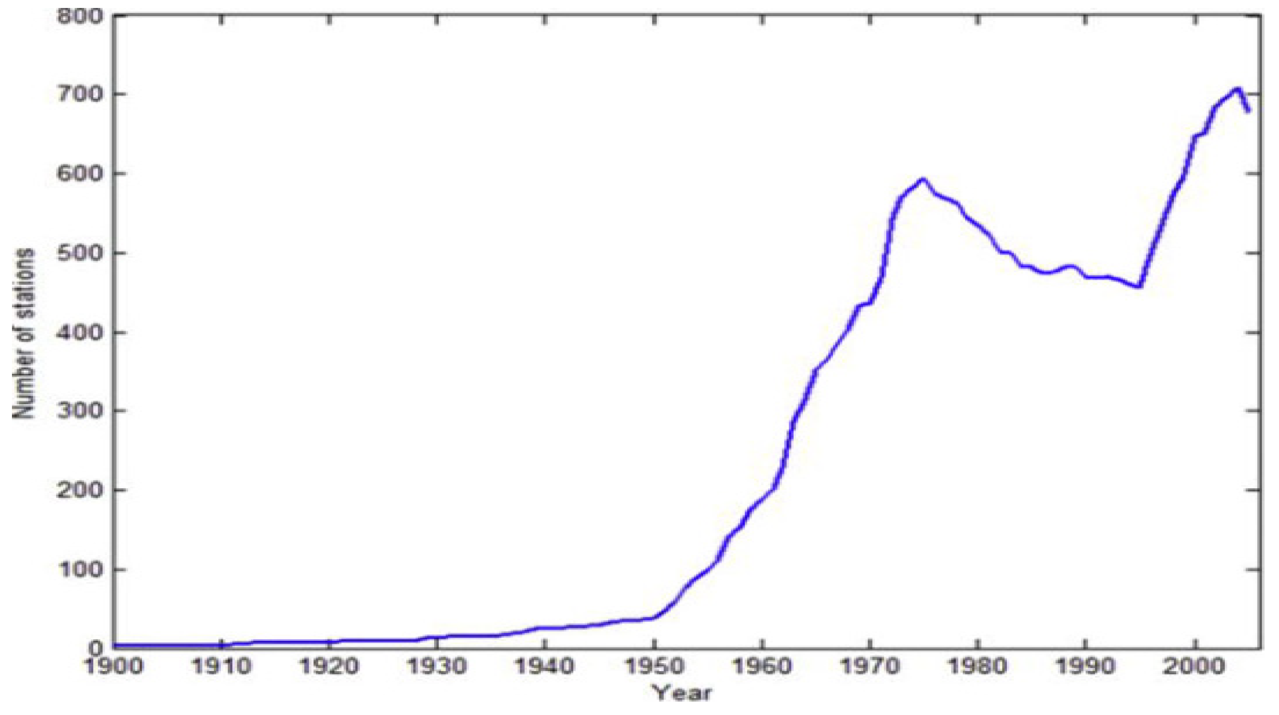
Figure 2.
Location of the Gowrie Creek catchment and details of the sub-daily rainfall data used in the rainfall disaggregation.
Figure 2.
Location of the Gowrie Creek catchment and details of the sub-daily rainfall data used in the rainfall disaggregation.
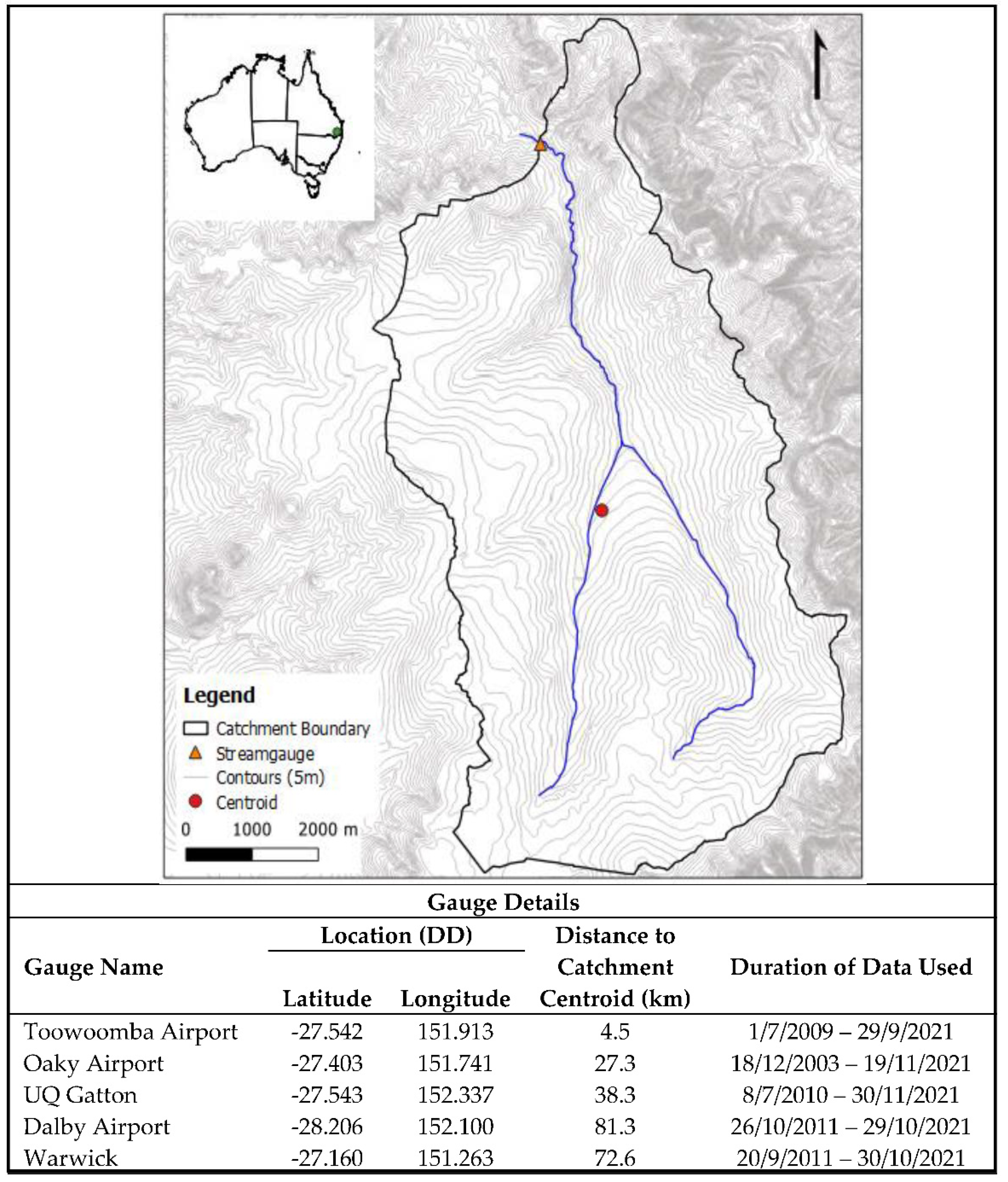
Figure 3.
Graphical representation of the 100 years of daily rainfall data sourced for this research (Jeffrey et al., 2001).
Figure 3.
Graphical representation of the 100 years of daily rainfall data sourced for this research (Jeffrey et al., 2001).
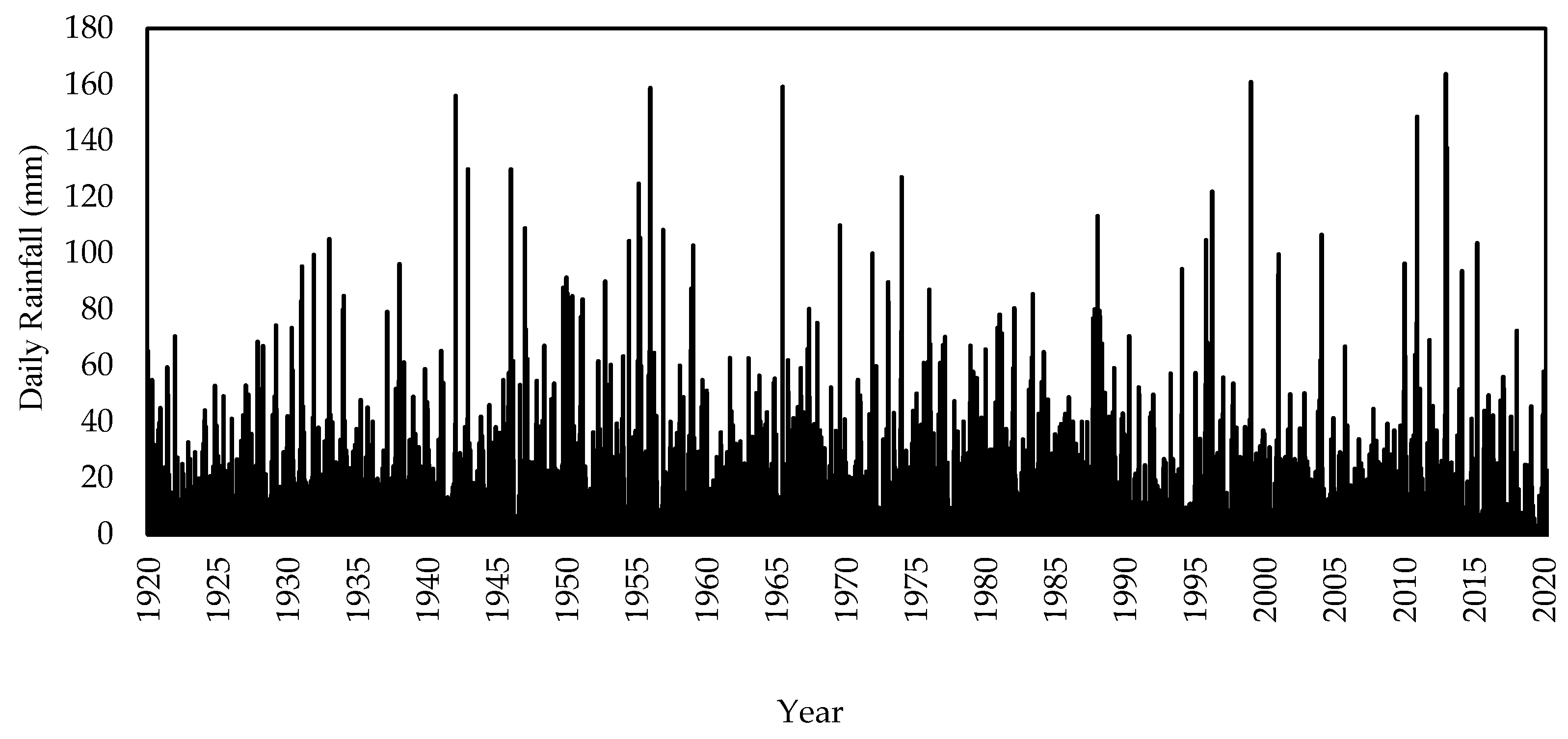
Figure 4.
Comparison of the MoF generated rainfall depths with the Bureau of Meteorology generated rainfall depths for the same duration and annual exceedance probability for three storm class options. Class option 2 shows the best fit, with the 1 in 1 line representing a perfect fit.
Figure 4.
Comparison of the MoF generated rainfall depths with the Bureau of Meteorology generated rainfall depths for the same duration and annual exceedance probability for three storm class options. Class option 2 shows the best fit, with the 1 in 1 line representing a perfect fit.
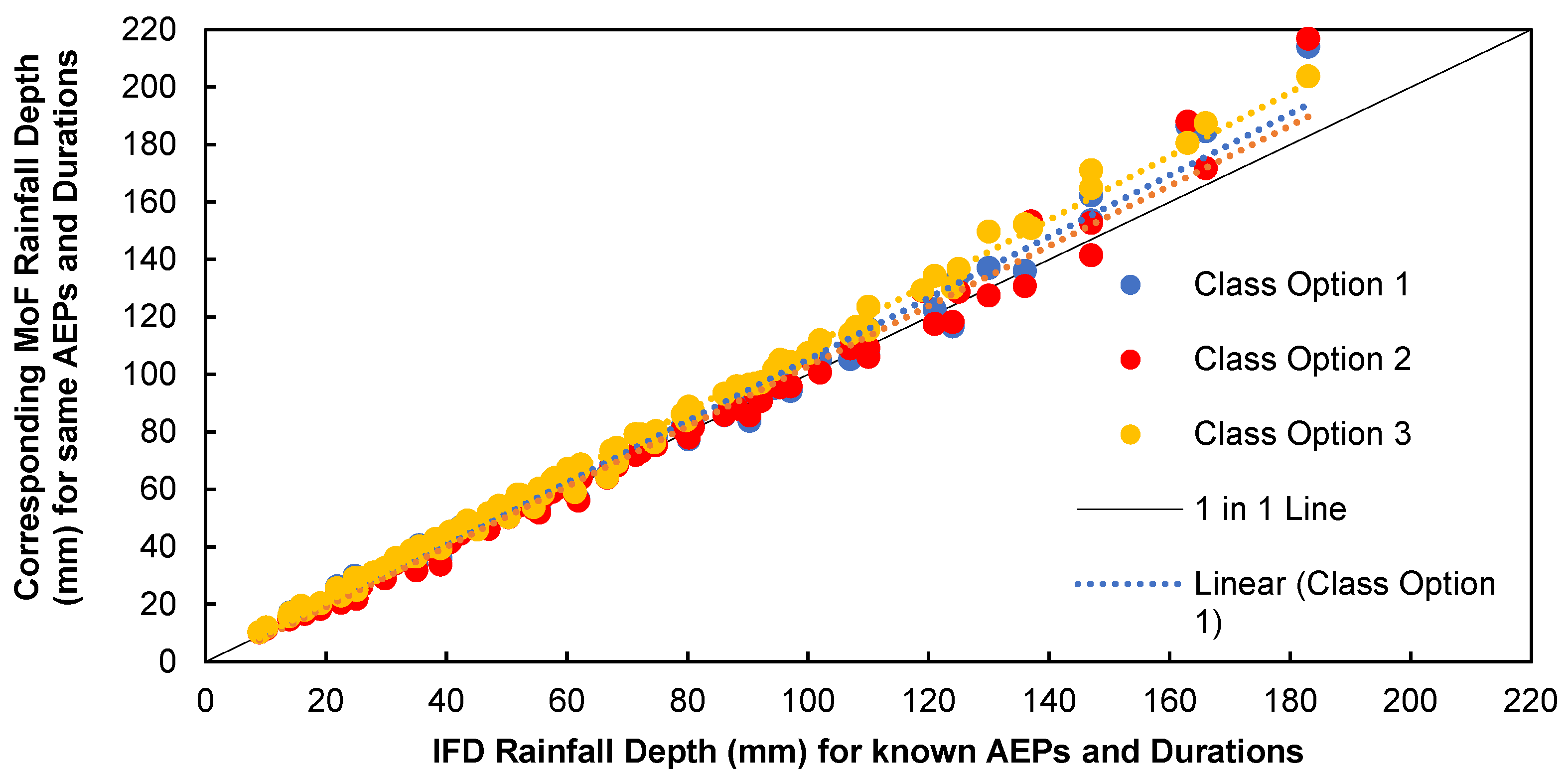
Figure 5.
Number of unique storms available for selection within each Class ID. Ignoring seasonality from the disaggregation process allowed for a much larger number of storms available for selection when using the MoFs.
Figure 5.
Number of unique storms available for selection within each Class ID. Ignoring seasonality from the disaggregation process allowed for a much larger number of storms available for selection when using the MoFs.
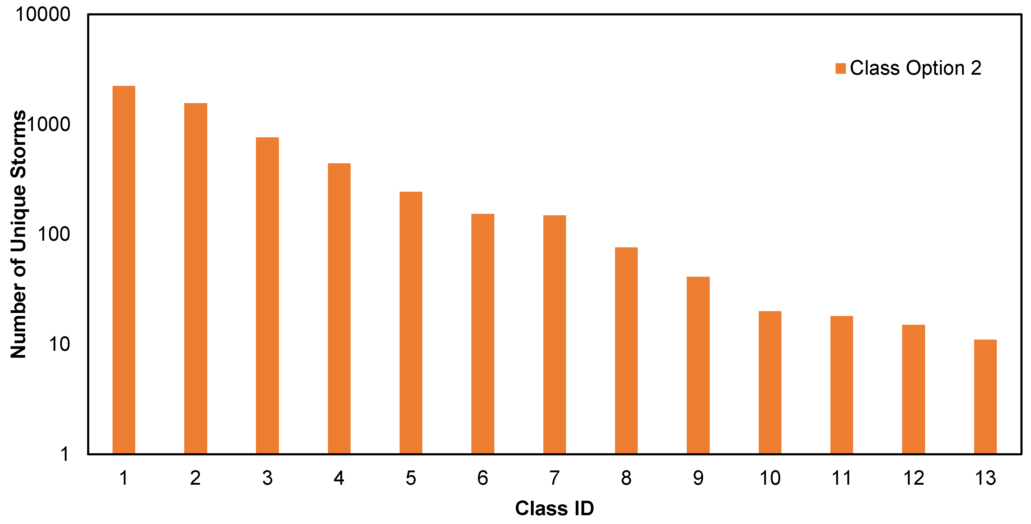
Figure 6.
Peak monthly flow from 100 years of continuous flow ranked in ascending order, with clear changes in trend highlighted by the red dots. A threshold value of 70 m3/s was used in this research based on this method.
Figure 6.
Peak monthly flow from 100 years of continuous flow ranked in ascending order, with clear changes in trend highlighted by the red dots. A threshold value of 70 m3/s was used in this research based on this method.

Figure 7.
Flood frequency analysis of all 20 simulations (orange), with the median result shown in black and the same analysis of the stream gauge series shown in green. The simulated results show a relatively tight range suggesting there is limited uncertainty in the result.
Figure 7.
Flood frequency analysis of all 20 simulations (orange), with the median result shown in black and the same analysis of the stream gauge series shown in green. The simulated results show a relatively tight range suggesting there is limited uncertainty in the result.
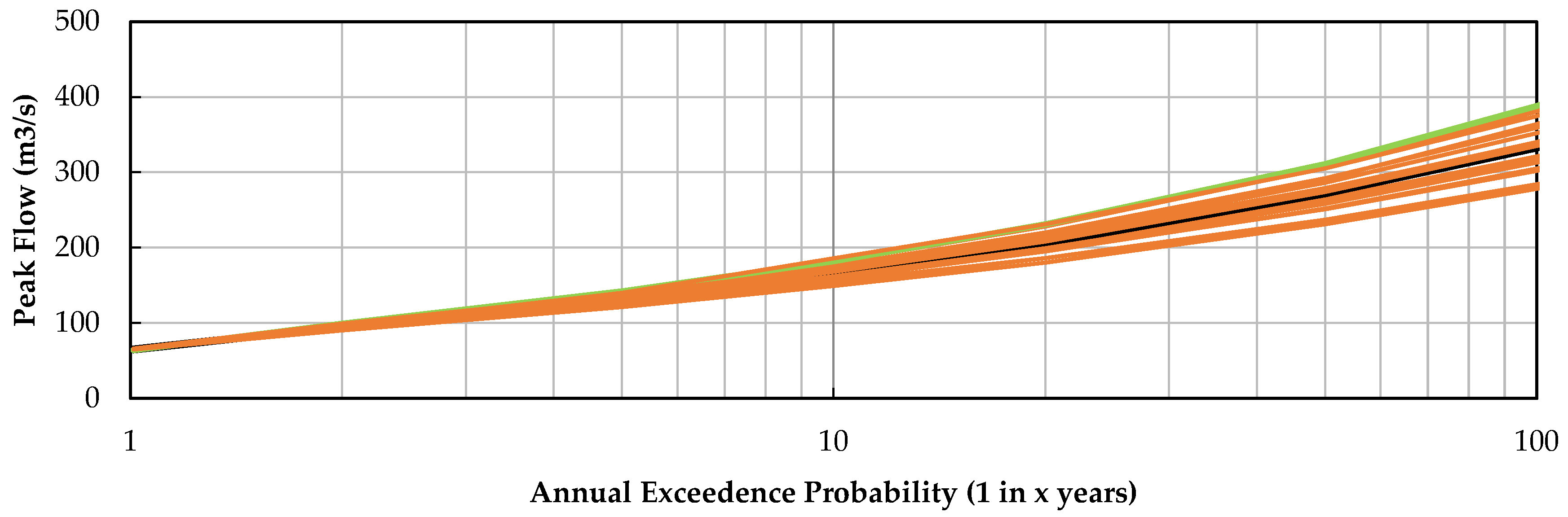
Figure 8.
Flood frequency analysis of 52 years of all 20 simulations (orange) with the median result shown in black, and the same analysis of the stream gauge series shown in green. The simulated results show a relatively tight range, suggesting that there is limited uncertainty in the result.
Figure 8.
Flood frequency analysis of 52 years of all 20 simulations (orange) with the median result shown in black, and the same analysis of the stream gauge series shown in green. The simulated results show a relatively tight range, suggesting that there is limited uncertainty in the result.
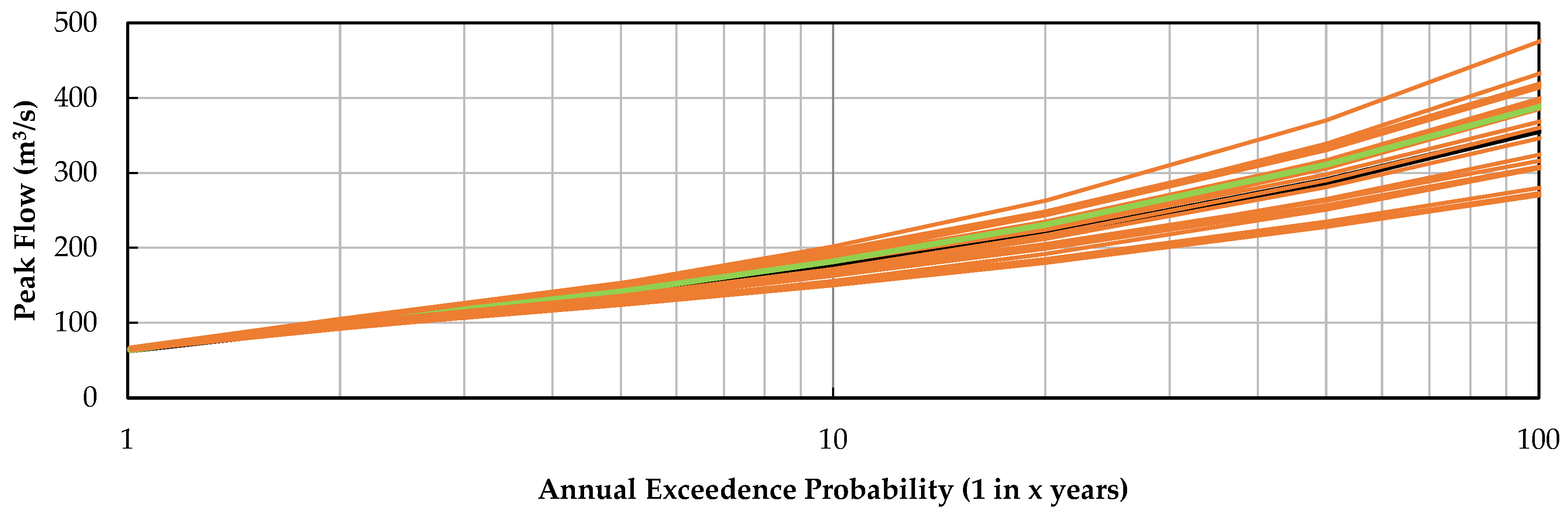
Figure 9.
Flood frequency analysis of different 50 year time periods of one model simulation. The results show a significant difference in the estimated peak flows based on the period of data adopted.
Figure 9.
Flood frequency analysis of different 50 year time periods of one model simulation. The results show a significant difference in the estimated peak flows based on the period of data adopted.
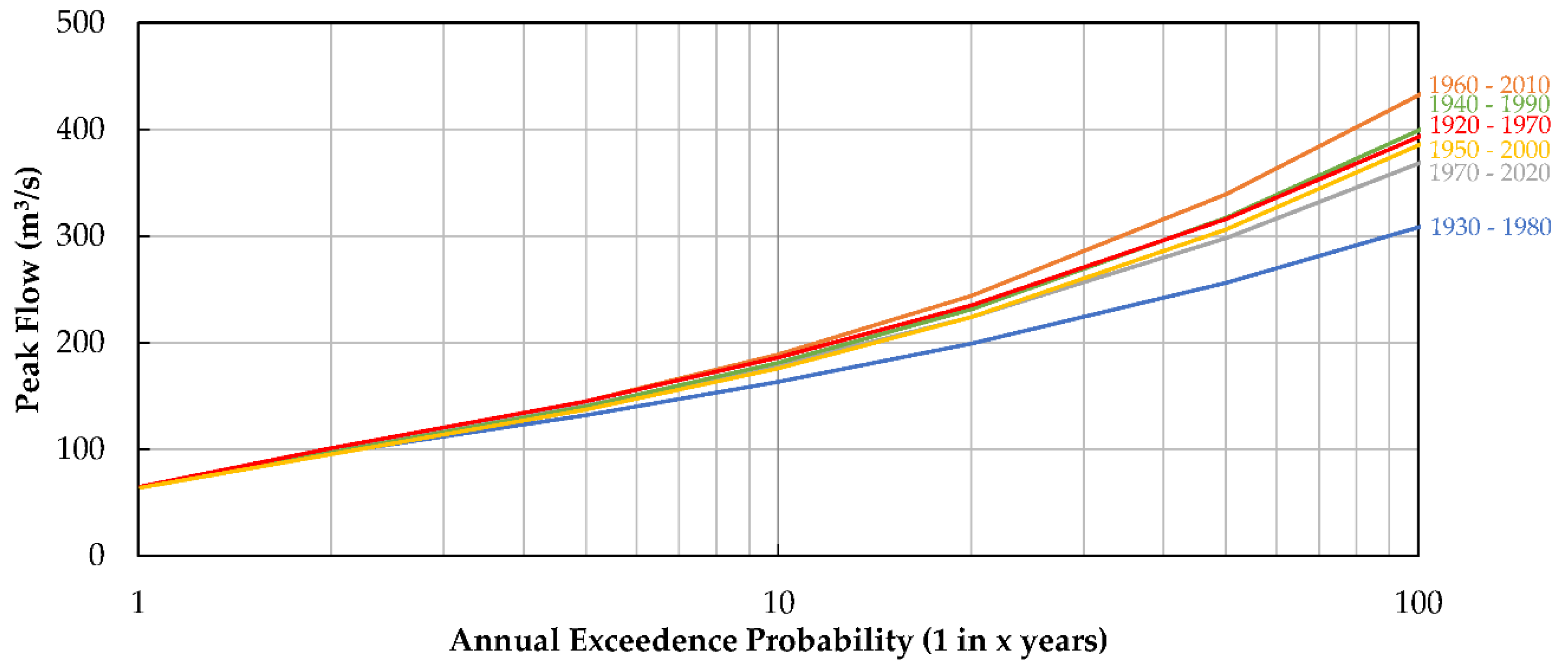
Figure 10.
Flood frequency analysis of all 20 simulations using the peaks over threshold series (orange) and annual maximum series (blue). In general, the annual maximum series results in higher peak flows for the same AEP while also resulting in a wider range (or increased uncertainty) in the results.
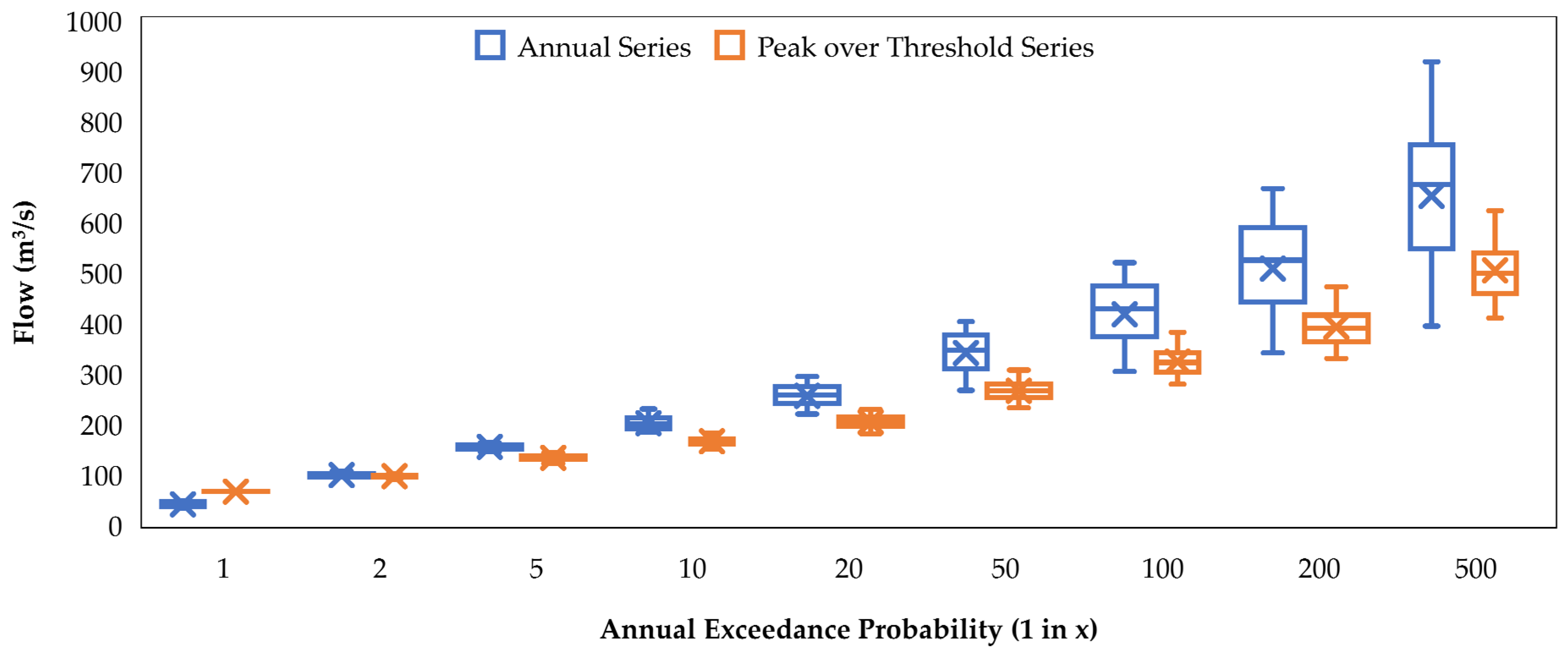
Figure 11.
Change in median peak flow (red) and range (black) for the 1% AEP with an increase in the number of disaggregated rainfall iterations. There appears to be a trend change in both results after 11 iterations.
Figure 11.
Change in median peak flow (red) and range (black) for the 1% AEP with an increase in the number of disaggregated rainfall iterations. There appears to be a trend change in both results after 11 iterations.
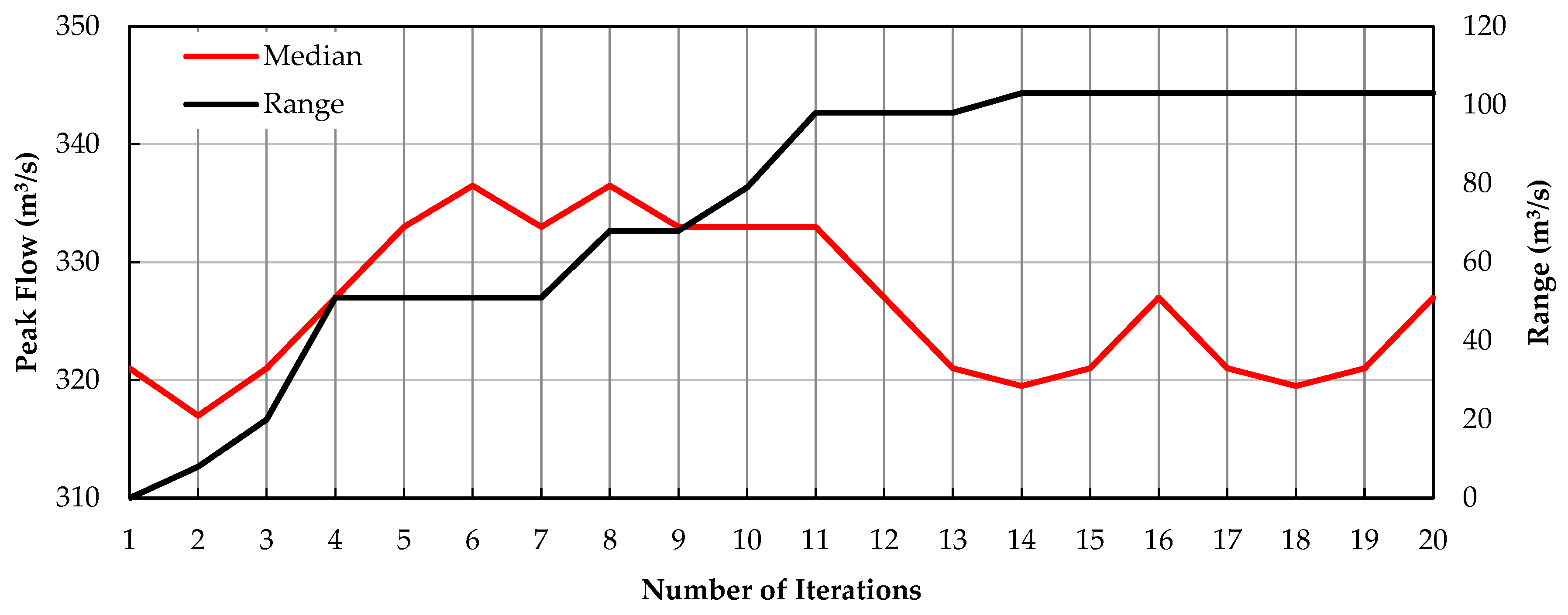
Figure 12.
Comparison of the results of this research (diamond) against the design event method (circle), the Rational Monte Carlo framework (cross) and a flood frequency analysis of the stream gauge. The comparison shows a good agreement between this research and the design event method.
Figure 12.
Comparison of the results of this research (diamond) against the design event method (circle), the Rational Monte Carlo framework (cross) and a flood frequency analysis of the stream gauge. The comparison shows a good agreement between this research and the design event method.
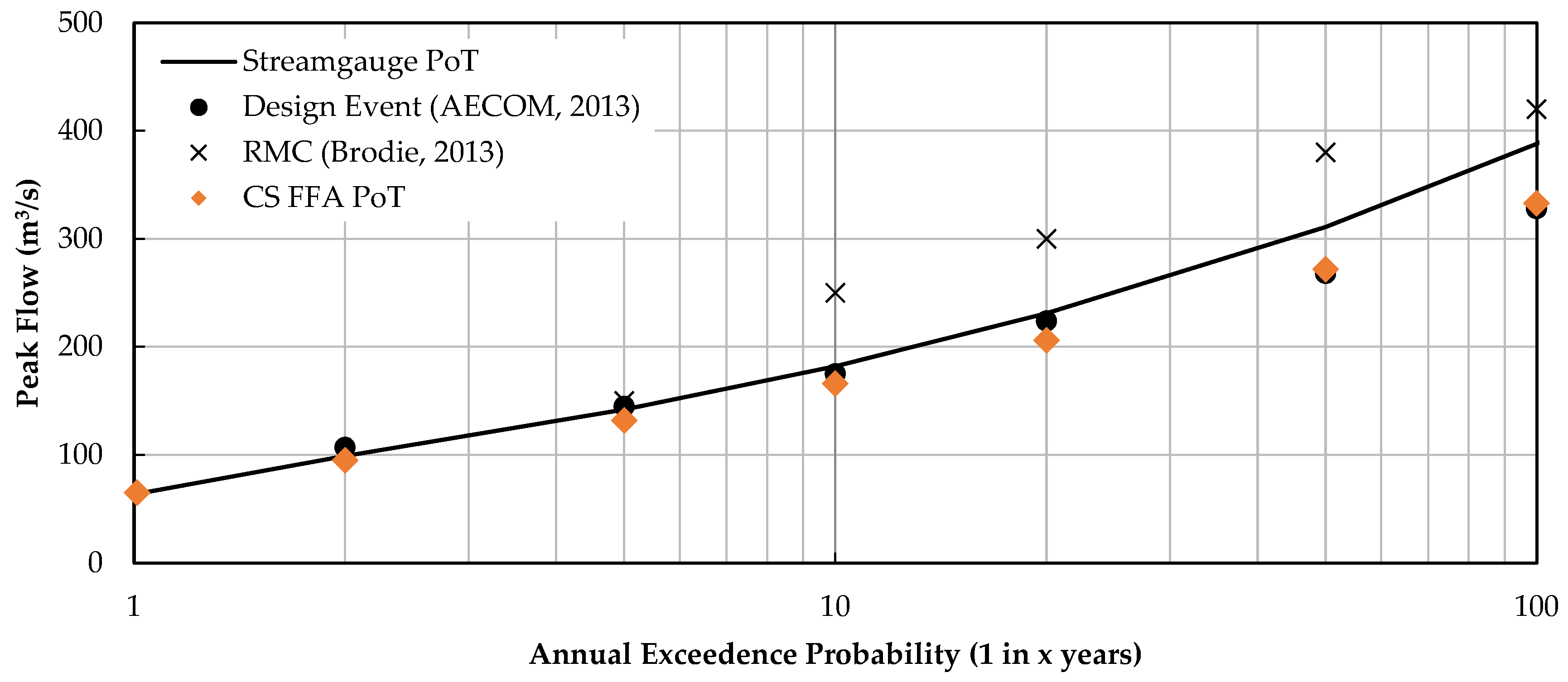
Figure 13.
Hydrographs for all scenarios simulated (red) for the major January 2011 event in comparison to the recorded stream flow (black).
Figure 13.
Hydrographs for all scenarios simulated (red) for the major January 2011 event in comparison to the recorded stream flow (black).
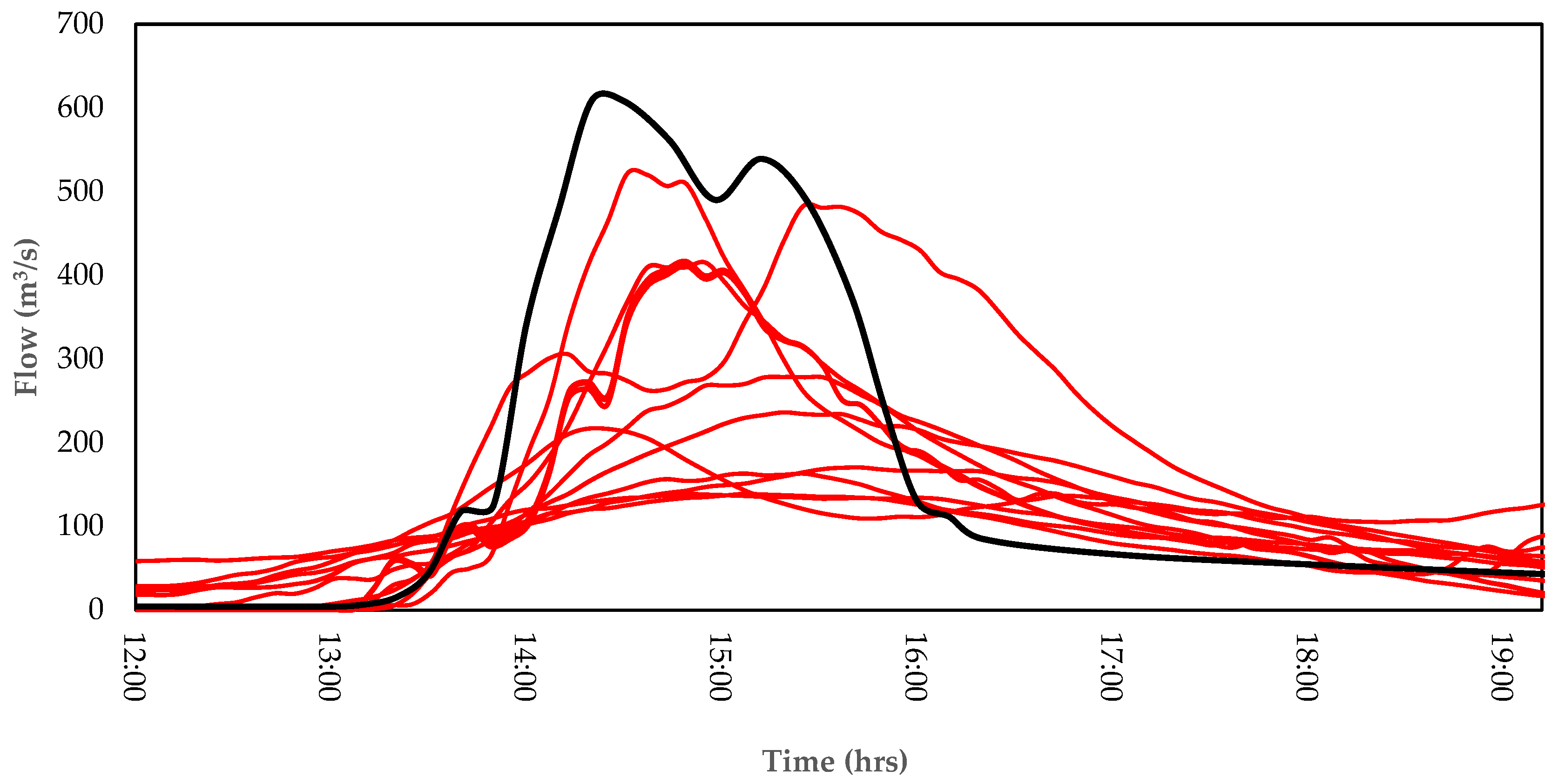

Table 1.
Storm class options assessed.
| Class ID | Option 1 | Option 2 | Option 3 | |||
|---|---|---|---|---|---|---|
| Min Rain (mm) | Max Rain (mm) | Min Rain (mm) | Max Rain (mm) | Min Rain (mm) | Max Rain (mm) | |
| 1 | 0.1 | 1 | 0.1 | 1 | 0.1 | 1 |
| 2 | 1.1 | 5 | 1.1 | 5 | 1.1 | 6 |
| 3 | 5.1 | 10 | 5.1 | 10 | 6.1 | 11 |
| 4 | 10.1 | 15 | 10.1 | 15 | 11.1 | 16 |
| 5 | 15.1 | 20 | 15.1 | 20 | 16.1 | 19 |
| 6 | 20.1 | 25 | 20.1 | 25 | 19.1 | 24 |
| 7 | 25.1 | 30 | 25.1 | 35 | 24.1 | 36 |
| 8 | 30.1 | 35 | 35.1 | 45 | 36.1 | 68 |
| 9 | 35.1 | 40 | 45.1 | 55 | 68.1 | 200 |
| 10 | 40.1 | 45 | 55.1 | 65 | ||
| 11 | 45.1 | 50 | 65.1 | 75 | ||
| 12 | 50.1 | 55 | 75.1 | 100 | ||
| 13 | 55.1 | 60 | 100.1 | 200 | ||
| 14 | 60.1 | 65 | ||||
| 15 | 65.1 | 70 | ||||
| 16 | 70.1 | 75 | ||||
| 17 | 75.1 | 80 | ||||
| 18 | 80.1 | 100 | ||||
| 19 | 100.1 | 200 | ||||
Disclaimer/Publisher’s Note: The statements, opinions and data contained in all publications are solely those of the individual author(s) and contributor(s) and not of MDPI and/or the editor(s). MDPI and/or the editor(s) disclaim responsibility for any injury to people or property resulting from any ideas, methods, instructions or products referred to in the content. |
© 2023 by the authors. Licensee MDPI, Basel, Switzerland. This article is an open access article distributed under the terms and conditions of the Creative Commons Attribution (CC BY) license (http://creativecommons.org/licenses/by/4.0/).
Copyright: This open access article is published under a Creative Commons CC BY 4.0 license, which permit the free download, distribution, and reuse, provided that the author and preprint are cited in any reuse.


