
Submitted:
04 August 2023
Posted:
09 August 2023
You are already at the latest version
Abstract
Bipolar disorder is a severe mood disorder and is one of the top 20 reasons of disability in the world. It causes a huge burden on society. In this study, the prediction models of bipolar disorder were constructed based on the concept of knowledge distillation. The input data consisted of patients of bipolar disorder and matched controls, all of which were selected from the open database MIMIC. The method of kernel density estimation (KDE) was exploited to generate probability density functions (PDF) which identify distributions of input data. The PDF values referred to as the soft labels were combined with the input data to construct the prediction models of bipolar disorder using decision tree and artificial neural network respectively. According to the evaluation results, indicators for identifying positive samples of bipolar disorder were improved. Meanwhile, the indicators for identifying negative samples have also been advanced. In addition, the branching attributes selected by the decision trees can be mapped back to specific disease diagnoses, which are all associated with bipolar disorder. In conclusion, using KDE to generate the soft label information of the input data can make knowledge distillation work and has improved the performances of prediction models for bipolar disorder.
Keywords:
bipolar disorder
; knowledge distillation
; kernel density estimation
; Medical Information Mart for Intensive Care (MIMIC)
; decision tree
; artificial neural network
1. Introduction
Bipolar disorder is a severe mood disorder characterized with alternating episodes of depression and mania [1,2]. During periods of mania, patients may exhibit unusually energetic, happy, or irritable behavior, and have reduced sleep. During depression, patients may cry inexplicably, have a negative attitude toward life, and have poor eye contact with others. According to statistics, 6% of patients with bipolar disorder die by suicide, and another 30-40% suffer from self-harm. Many patients with bipolar disorder also suffer from other mental illnesses, such as substance abuse addiction, anxiety disorders, etc. According to academic researches, people with bipolar disorder account for about 1% of the global population [3]. In the United States, approximately 3 percent of the population experience bipolar symptoms at some points in their lives, with no significant gender differences [4]. The most common age for onset of symptoms is between 20 and 25 years old. The younger the age, the worse the prognosis [5].
The combined action of many genetic variations may lead to the development of bipolar disorder [1], and genetic factors account for about 70-90% of the risk of bipolar disorder [6,7]. Environmental risk factors include the history of childhood abuse and chronic stress [1]. In addition, many other psychiatric disorders share symptoms of bipolar disorder, including attention deficit/hyperactivity disorder, schizophrenia, substance abuse, etc. [1]. On the other hand, about one-quarter to one-third of people with bipolar disorder experience economic, social, or professional problems [1]. According to the survey provided by WHO, bipolar disorder is one of the top 20 reasons of disability in the world, and causes a huge burden on society [8]. Moreover, some diseases have a higher incidence in patients with bipolar disorder compared to the general population, including coronary heart disease, metabolic syndrome, migraine, obesity, and type 2 diabetes. Accordingly people with bipolar disorder have twice the risk of death compared to the general population [1,5]. For a recent study conducted between January 2018 and January 2020 at a hospital in Turkey, each of the 1148 patients with bipolar disorder was interviewed to investigate the incidence of various target diseases in his/her first- and second-degree relatives as well as himself/herself. It was found that if there is a family history of epilepsy, the patient's symptoms of mental illness will be more pronounced. Similarly, a family history of diabetes mellitus is strongly associated with bipolar disorder, and a family history of thyroid disease is correlated with co-occurring anxiety disorders. Finally, there exists a co-morbid association between bipolar disorder and cerebrovascular disease [9].
There is an intuitive way to improve the performance of machine learning. Different models can be trained respectively using the same dataset, then their prediction outcomes will be integrated. However, such ensemble learning may consume computational resources. Moreover, for deep neural networks trained on images, it has been generally observed that the learned features are similar to Gabor filters and color patches. Therefore, the concept of transfer learning is proposed. In the applications of computer vision, the technique of transfer learning is constantly used in problems such as object detection and target segmentation. A common practice for transfer learning is to train a basic convolutional neural network using the input dataset firstly. Then its convolutional layers, the earlier layers of the network architecture, and/or the connection weights, are duplicated in the target network [10,11]. Similar to the concept of transfer learning, the idea of “knowledge distillation” is proposed and its effectiveness has been verified in various studies. For the practice of knowledge distillation, firstly a sophisticated model or multiple models will be trained using any learning algorithm, such as the deep neural network. Outcomes produced by this group of “teacher models” can be thought of as conditional distributions for the input data, and may be referred to as “soft labels”. These data distributions can be used as the learning targets for the “student model”, which will be trained using simpler learning architectures [12,13]. The evaluation results have shown that the student model with a simpler architecture can achieve prediction performances close to those produced by complex learning architectures. On the other hand, the soft labels can be used as the reference information and to train the student model together with the original input data. This process may also be seen as the student model "distilling" the "knowledge" provided by the group of teacher models [14].
The kernel density estimation (KDE), which is a nonparametric estimation approach in statistics, has been widely exploited to identify distributions in various types of datasets. A kernel density estimator generates an approximate probability density function (PDF) by computing the linear combination of the weighted kernel functions placed at the locations of all data instances in the vector space. Accordingly, variations in the vector space with different PDF values can be identified as distributions of data instances [15,16,17]. In this article, we will report how the KDE method performed with a real medical dataset and how it has been exploited to identify distributions hidden in the data. Moreover based on the concept of knowledge distillation, the PDF values produced by the KDE method were then transferred as the soft labels to construct the prediction models of bipolar disorder using learning methods of decision tree and artificial neural network respectively. According to the evaluation results, using the data distribution information generated by KDE has improved the true positive rates and positive predictive values, meanwhile the indicators for identifying negative samples were also advanced. In addition, the branching attributes selected by the decision trees have been mapped back to specific disease diagnoses, which are all associated with bipolar disorder. To the best of our knowledge, this study is the first attempt to apply KDE to knowledge distillation for supervised machine learning.
2. Materials and Methods
2.1. The input data
In the early 2000s, the "Laboratory for Computational Physiology" of the Massachusetts Institute of Technology (MIT) began to implement the project "Integrating Signals, Models and Reasoning in Critical Care". The main goal of this project is to build a large dataset for researches based on intensive care, the result of which is the database "Medical Information Mart for Intensive Care, (MIMIC)". The contents of this database come from Beth Israel Deaconess Medical Center (BIDMC). MIMIC is a publicly shared medical database. It contains de-identified information from electronic medical records for thousands of adult patients admitted to medical/surgical intensive care units and emergency wards. The development of this database is approved by the ethical review boards of BIDMC and MIT, respectively. MIMIC has been used extensively by academic researchers around the world, helping to promote advances in clinical informatics, epidemiology, and machine learning [18].
In the database tables of MIMIC, all the information of the same patient are concatenated with the field value of “subject_id”. In this case-control study, the case group included patients with bipolar disorder and/or related symptoms. The following diagnostic codes were used when selecting case samples from the table “diagnoses_icd”. Their ICD-9 versions are 296.40~296.45, 296.50~296.56, 296.60~296.62, 295, 298; ICD-10 versions are F20, F29, F31. Then 10,000 people were randomly selected from these patients of bipolar disorder to form the case group. The date of the firstly diagnosed bipolar disorder for each case patient, i.e. the field value of “admittime”, was regarded as the index date. Finally for each case patient, the subject_id was used to retrieve all his/her diagnosis records in the database.
On the other hand, the control sample did not have diagnoses of bipolar disorder and any associated symptoms in the database. They were matched with the case patients in age and gender, i.e. the field values of “gender” and “anchor_age” from the table “patients”. In addition, in the month of the index date for a case patient, the corresponding control sample must have any diagnosis record, which represents similar health status. Based on the aforementioned matching conditions, this study selected the control samples at a ratio of 1 vs. 1 and 1 vs. 3, respectively. Finally for each control sample, the subject_id was used to retrieve all his/her diagnosis records in the database to form the input data.
2.2. Kernel density estimation
Kernel density estimation (KDE) is the application of kernel smoothing for probability density estimation, i.e., a non-parametric method to estimate the probability density function of a random variable based on kernels as weights [15,16]. KDE answers a fundamental data smoothing problem where distributions about the population are made [17]. For the basic definition of KDE, let (x1, x2, …, xn) be independent and identically distributed samples drawn from a specific distribution with an unknown density f at any given point x. Its kernel density estimator can be defined using Formula (1).
In Formula (1), K(x-xi; h) is the kernel function, whose outcomes are non-negative values. There exists a range of kernel functions being used, such as cosine, linear, normal, etc. [15,16]. The positive variable h is called the bandwidth, which is a smoothing parameter and exhibits a strong influence on the resulting estimation. In this study, the class of “KernelDensity” from the scikit-learn package was used to perform the KDE analyses. After verification, the exponential kernel (i.e. K(x; h) = exp()) was chosen to estimating distributions of input data for subsequent computations of knowledge distillation. The smoothing parameter h was set to 0.2, which is the default value given by the scikit-learn package.
2.3. Embedding vector
In the application of machine learning, the content of category data needs to be converted into a special format before subsequent analyses can be performed. In addition to transforming them into numerical information, these representations should correctly retain the characteristic attributes of the original data contents. The idea of embedding vector will present a categorical data item (such as a word in a text) in the form of a multi-dimensional vector. Each element of the vector is a real number, and the contents of the vector can reveal the properties of the original data items [19]. The embedding vector can be generated by the parameter optimization mechanism using a specific neural network architecture [20,21]. As for the loss function required in the learning process, its basic concepts are defined as Formula (2).
Formula (2) represents the conditional probability of correctly judging the context (i.e. m words before and after wi, which constitute contents in the sliding window as wi-m, ……, wi-1, wi+1, ……, wi+m) with the word vector wi as the input premise. The probability value can be increased as much as possible through the parameter optimization mechanism. Then sum up the conditional probability values of all the words in the full text (e.g. a total of N words), and the logarithm function is used to simplify the computation process. The expected loss function is shown in Formula (3).
When implementing the program suite of this loss function, the data structure of the Huffman tree can be used to improve the computational performance.
The "word2vec" proposed by Google in 2013 is currently the mainstream embedding vector algorithm [20,21]. The algorithm combines two learning mechanisms: skip-gram and CBOW (continuous bag of words). In the calculation of skip-gram, the word vector wi is used as the input premise, and the predictions of m word vectors before and after wi, which constitute contents in the sliding window as wi-m, ……, wi-1, wi+1, ……, wi+m, are respectively produced. On the other hand, in the computation of CBOW, the 2m word vectors within the sliding window, i.e. wi-m, ……, wi-1, wi+1, ……, wi+m, are used as the input premises, and the prediction of the word vector wi is outputted.
2.4. Machine learning algorithms
The decision tree is a hierarchical model that uses a tree-like structure. In this model, each internal node represents a test on an attribute, and each branch represents the outcome of the test. At the bottom of the structure, each leaf node represents a class label, which is the decision taken after analyzing all of the attribute features [22]. The path from the root note to a leaf represents a specific decision rule, and the conditions along the path form a conjunction of “if-then” clauses [23]. The decision tree is a white-box model because the decision rules produced are easy to understand and interpret. The node branching function used can have an impact on improving the accuracy of the decision tree. Among various types of node branching functions, the Gini impurity is constantly used and was chosen in this study. According to the relative frequencies of class labels in the dataset, the Gini impurity measures how often a data item will be incorrectly labeled if it was labeled randomly and independently. For a dataset of items with J class labels and relative frequencies pi, i ∈ {1, 2, …, J}, the probability of correctly recognizing the class label of a data item, assuming it is class i, is pi. On the contrary, the probability of misclassifying that item is . Therefore, the computation formula of Gini impurity IG(p) is defined as follows.
IG(p) reaches the minimum value zero when all data items in the node fall into a single class label.
The artificial neural network is a machine learning algorithm that imitates the human nervous system, and its definition formula is as follows [24,25].
Because the neural network can have a plurality of input and output neurons, they will be assembled respectively into the "input layer" and the "output layer". The matrix X represents the input values of a set of attributes, and the matrix Y simulates the output neurons for the computation results. The weight matrix W simulates the axons, which connect the input/output neurons and are responsible for transmitting messages. In the application problem, this represents the respective influences of different attribute characteristics. The matrix B of bias values simulates synapses and represents the degree to which the output neurons are activated. The higher the bias values are, the easier it is for a neuron to be activated and transmit the message. The symbol represents the activation function, which accepts a weighted sum of input values and performs a special calculation. If the resulting value is greater than the threshold, the output neuron is activated and the message is transmitted. In addition, the "hidden layer" can be added to the network architecture, containing nodes that mimic internal neurons. Since the hidden layer makes the network structure more complicated, it can handle more kinds of application problems, or simulate the interaction of more complex attribute features.
2.5. The analysis procedure
This study used the concept of knowledge distillation to construct predictive models of bipolar disorder. After the case patients and control samples were screened from the MIMIC database, all of their diagnosis records in the database were selected as the input data. In the MIMIC database, an average of 20 different disease diagnoses are recorded for each sample. Using the aforementioned word2vec algorithm, these disease diagnoses were converted into 8-dimensional embedding vectors. Therefore, the input data of each sample would be stored in a 20×8 matrix structure. The research team then planned two analysis procedures as follows.
Referring to Figure 1a, in the first procedure the KDE was used to estimate the probability density function representing the distribution for the input data X. After the data X was input into the density function, the soft label information Xpdf was produced, which represented the likelihood values of the data distribution of the input X. Next, Xpdf was used as the input attributes of the training dataset, and the set Y contained the class labels as the learning targets. In this study, supervised learning methods such as decision tree and artificial neural network were used respectively to construct the predictive models for bipolar disorder.
Referring to Figure 1b, in the second analysis procedure the KDE method was still used to convert the input data X into the soft label information Xpdf. Next, both of X and Xpdf were used as the input attributes of the training dataset, and Y still was the set of class labels for learning. Finally, decision tree and artificial neural network were used respectively to develop the predictive models for bipolar disorder.
3. Results
The datasets of this study were composed of case patients of bipolar disorder and the matched control samples, with a ratio of 1:1 and 1:3, respectively. The distributions of these data would be computed using KDE to produce the corresponding probability density functions as the soft label information for subsequent knowledge distillation. When using a machine learning algorithm to construct the prediction model for bipolar disorder, the randomly selected 80% of data samples would be used for model training and validation, and the remaining 20% were used as the testing set. When estimating the data distributions with KDE, we used the exponential kernel function. In addition, we set Gini impurity as the branching function for constructing the decision tree. When training the prediction models with artificial neural network, we chose ReLU and sigmoid respectively as the activation functions of the network nodes. Finally, cross entropy and Adam optimizer were set as the loss function and optimization mechanism respectively when training and validating the prediction models with artificial neural network.
In the following paragraphs of this paper, we define a specific sequence to express the architecture of the neural network. Assuming that the architecture contains three hidden layers, and the number of nodes in each hidden layer is v1, v2, and v3 respectively, then we use NN(v1, v2, v3, 1) to represent architecture of this neural network. Since the learning models in this study are all binary predictors of bipolar disorder, the last 1 in the sequence represents only one node in the output layer. There have been three types of network architecture evaluated in this study: NN(80, 10, 1), NN(160, 40, 1), and NN(80, 20, 10, 1). All of these architectures were tested and verified empirically.
Because the learning models in this study are all binary predictors of bipolar disorder, we adopt the terminology from a confusion matrix: true positive (TP), true negative (TN), false positive (FP), and false negative (FN). The following metrics are utilized for evaluating performances of prediction models trained by various machine learning algorithms respectively.
For the dataset of case patients and control samples with the matching ratio of 1:1, their respective probability density functions estimated by KDE are presented in Figure 2 in the format of curve chart. Observing the content of Figure 2, we can find that the respective probability density functions of case patients and control samples are quite different. In other words, they exhibit very different data distributions in diagnostic records used as characteristic attributes.
Next, we have tried to test whether the data distribution information estimated by KDE is helpful for constructing the learning model. For our first analysis procedure (Figure 1a), the soft label information Xpdf, which represented the likelihood values of the data distribution of the input X, were used as the attributes for training and validating the prediction models. The evaluation results for the testing set are shown in Table 1a.
For our second analysis procedure (Figure 1b), both of X and Xpdf were used as the input attributes for training and validating the prediction models. The evaluation results for the testing set are shown in Table 1b.
Finally, in order to verify the effectiveness of the soft label information Xpdf, only the data X were used as the attributes for training and validating the prediction models. The evaluation results for the testing set are shown in Table 1c.
Comparing the results shown in Table 1a,c, only using the soft label information Xpdf as the input attributes does not always improve the performances of the predictive models. However, when both of X and Xpdf are used for training and validating the prediction models (Table 1b), not only the TPR and PPV are improved, but also the TNR and NPV become better.
In order to confirm that the data distributions generated by KDE can play a role in knowledge distillation, we repeated 10 times to randomly select case patients and matched control samples to form the dataset. Each time we used KDE to generate the soft label data Xpdf, and then the Xpdf were utilized to train a decision tree. Finally we examined the decision rules accompanying the tree structure and counted the features in Xpdf most frequently chosen as branching attributes. According to the descending order of the chosen frequency, the disease diagnoses corresponding to these branching attributes are listed below.
For decision rules leading to the positive label of bipolar disorder, the most frequent branching attributes include: hypertension; depressive disorder; anxiety disorder; suicidal ideations; type II diabetes mellitus; hyperlipidemia; esophageal reflux; chest pain; nicotine dependence; asthma; hypercholesterolemia; hypothyroidism; alcohol abuse.
For decision rules leading to the negative label of bipolar disorder, the most frequent branching attributes include: hypertension; hyperlipidemia; type II diabetes mellitus; chest pain; alcohol abuse; esophageal reflux; atrial fibrillation; hypercholesterolemia; depressive disorder; atherosclerosis/coronary heart disease; abdominal pain; urinary tract infection; hypothyroidism; nicotine dependence; headache; syncope and collapse.
For the dataset of case patients and control samples with the matching ratio of 1:3, their respective probability density functions estimated by KDE are presented in Figure 3 in the format of curve chart. Again it can be found that case patients and control samples exhibit very different data distributions in diagnostic records.
For this dataset, the evaluation results of the testing set on prediction models of bipolar disorder trained using various learning algorithms are presented in Table 2. Comparing the results shown in Table 2a,c, the prediction models using the soft label information Xpdf as the input attributes constantly perform worse than models trained using the input data X. However, when comparing the results shown in Table 2b,c, using both of X and Xpdf as the input attributes for training the prediction models improves all evaluation metrics.
Finally for the dataset of cases and controls with the matching ratio of 1:3, the decision tree analysis mentioned above has been executed again. Similarly we examined the decision rules accompanying the tree structures produced, and counted the features in Xpdf most frequently chosen as branching attributes. According to the descending order of the chosen frequency, the disease diagnoses corresponding to these branching attributes are listed below.
For decision rules leading to the positive label of bipolar disorder, the most frequent branching attributes include: hypertension; depressive disorder; anxiety disorder; suicidal ideations; type II diabetes mellitus; esophageal reflux; hyperlipidemia; nicotine dependence; hypercholesterolemia; asthma; chest pain; hypothyroidism; atherosclerosis/coronary heart disease.
For decision rules leading to the negative label of bipolar disorder, the most frequent branching attributes include: hypertension; hyperlipidemia; type II diabetes mellitus; esophageal reflux; chest pain; depressive disorder; alcohol abuse; hypercholesterolemia; atherosclerosis/coronary heart disease; atrial fibrillation; nicotine dependence; hypothyroidism; chest pain; headache; urinary tract infection; abdominal pain; syncope and collapse.
4. Discussion
In the evaluation results of this study, the predictive performances of the models trained only with soft label information Xpdf are not always better than those of the models trained with only input data X (Table 1a,c)). Moreover, we can also observe trade-offs between PPV and TPR values when increasing the sample size of matched controls, i.e. from 1:1 to 1:3. In other words, comparing the prediction results of the models trained with Xpdf and X respectively on the testing set, we have found that the increase in PPV values is accompanied by the decrease in TRP values, or vice versa (Table 2a,c)). In addition, increasing the sample size the matched controls means that the input data of the negative class increases, so the evaluation indicators NPV and TNR of the prediction models to identify negative testing samples will be improved (Table 1 and Table 2). Regardless of the matching ratio of case patients and control samples, we can observe that as long as the soft label information Xpdf are combined with the input data X to train the prediction models, the evaluation indicators PPV and TPR for identifying positive testing samples will be improved. At the same time, the indicators NPV and TNR for identifying negative samples have also been advanced (Table 1 and Table 2). To sum up, this study used KDE algorithm to generate the soft label information Xpdf which can make knowledge distillation work and may improve the predictive performances of the trained models.
In order for knowledge distillation to improve the prediction performance of the trained model, the soft label information must provide accurate distribution conditions of the input data. Referring to the research work of G. Hinton et al, they argued that adding a "temperature" variable to the formula that normalizes the predicted outputs can smoothening the probability distributions for the class labels. Moreover, the research team proposed to use the probability distribution values produced by the sophisticated deep learning model as the soft label. Input these reference information together when training a shallow neural network model can achieve prediction accuracies close to those of sophisticated deep learning models. They concluded that the “knowledge” of a deep learning model can be transferred to a shallow “distilled” learning model [14]. In addition, the parameter optimization of artificial neural network can adopt the concept of conditional probability. Under the premises of input data and current parameter settings, the predicted conditional probability distributions can approximate the true distributions of class labels. A typical solution for this problem is the Monte Carlo approximation. However, this method needs to construct multiple sets of prediction models and store multiple sets of parameter settings. Consequently more computing resources are required. In view of this, the research work of A. Korattikara Balan et al proposed an improvement. Firstly, sample data are selected to construct multiple models of different neural networks. These network models form the "teacher group" for ensemble learning. The group of teachers produce sets of outcomes, which were presented as the conditional probability distributions. These probability distributions were used as the learning targets for the "student" neural network. The parameters of the student network model are optimized through the training process. Therefore, the final outcomes of the student network, which are also presented as probability distributions, can be thought of as approximating the conditional probabilities provided by the teacher group. The approach proposed by this work also amounts to the student network “distilling” the knowledge provided by network models of the teacher group [12]. On the other hand, essentially KDE is a non-parametric method of estimating distributions of data samples. It is known that KDE has been applied in estimating the conditional probability distributions of input data when using a naive Bayes classifier [17,26]. Referring to the contents of the aforementioned literatures, this study was inspired to combine KDE for knowledge distillation to construct prediction models for bipolar disorder.
When KDE is used for data analysis, it often focuses on the setting of bandwidth. This parameter has a great influence on the accurate estimation of data distributions. If the set value of bandwidth is too small, the under-smoothed distribution will contain many spurious data artifacts. On the contrary, if the value of bandwidth is set too large, the over-smoothed distribution will obscure much of the underlying structures. There has been numerous studies discussing the criteria to set this parameter [15,16,27]. A novel KDE method developed by our research team has been exploited to identify interesting patterns hidden in the dataset. The main features of this method include minimizing the bias part of the mean square error, and elevating the bandwidths of the kernel functions to alleviate the effects of variance. It has been verified that our novel KDE can estimate the distributions of input data more accurately than many traditional KDE methods [28,29,30,31]. Therefore, one of our future works will use this novel KDE for knowledge distillation to construct more accurate predictive models.
In order to further verify effectiveness of the soft label information Xpdf generated by KDE, we examined the decision rules of the tree structures constructed with Xpdf. Regardless of the matching ratio of case patients and control samples, we have found that identical disease diagnoses are selected as the branching attributes from the analysis results. The contents contained in Xpdf are not categorical disease descriptions, but likelihood values of the probability density functions generated by KDE. Therefore, the features selected as branching attributes in the decision rules must be mapped back to the categorical disease descriptions. Since identical disease diagnoses are always selected as the branching attributes, Xpdf do provide correct distribution information of the input data. On the other hand, through survey of reference literatures, we have found various associations between bipolar disorder and these disease diagnoses selected by the decision trees. It is known that 6% of patients with bipolar disorder die by suicide, and another 30-40% suffer from self-harm [1]. Many patients with bipolar disorder also suffer from other mental illnesses, such as anxiety disorders, schizophrenia, substance abuse, etc. Furthermore, one typical symptom of the depressive phase of bipolar disorder is fatigue [1]. Moreover, some diseases have a higher incidence in patients with bipolar disorder compared to the general population, including metabolic syndrome, migraine, obesity, and type II diabetes [5]. In addition, compared to the general population, patients with bipolar disorder have twice the risk of dying from coronary heart disease [1]. Meanwhile, hypertension, hyperlipidemia, hypercholesterolemia, chest pain, etc., are typical risk factors and symptoms of coronary heart disease.
Since bipolar disorder and asthma are leading causes of morbidity in the US, recently a cross-sectional analysis explored the clinical characteristics of bipolar disorder and an asthma phenotype and fitted a multivariable regression model. The evaluation results concluded that a history of asthma is common among patients with bipolar disorder [32]. Some medical illnesses with clinical presentations similar to symptoms of bipolar disorder, such as the similar features between migraine headache and bipolar disorder. Some symptoms also need to be identified whether they are caused by bipolar disorder or endocrine system diseases such as hypothyroidism or hyperthyroidism [33]. Another study conducted in Sweden has found that higher odds for bipolar disorder co-morbidity occurred in patients with gastroesophageal reflux disease [34]. Furthermore, recently a genome-wide pleiotropic association study using genome-wide association summary statistics concluded that the pleiotropic genetic determinants between gastrointestinal tract diseases and bipolar disorder are extensively distributed across the genome. The findings provide supports for the shared genetic basis underlying the gut-brain axis [35]. Referring to the research work of Benjamin J S Al-Haddad et al, a total of 1,791,520 Swedish children born between 1973 and 2014 were observed for up to 41 years using linked population-based registries. The analysis results suggested that fetal exposure to any maternal infection, such as urinary tract infection, while hospitalized increases the risks for autism and depression, but not bipolar or psychosis, during the child's life [36]. However, ketamine is mainly used for bipolar disorder, and it has been reported that longstanding ketamine abuse may cause urinary tract infection [37].
It is known that cerebrovascular reactivity (CVR) represents the relax ability of cerebral blood vessels to vasoactive substances, and is a quantitative indicator for cerebrovascular health. Results of the analysis performed by Adam L Urback's research team have shown that adolescents with bipolar disorder had lower CVR values in the posterior cingulate and periventricular white matter than the mentally healthy controls. After adjusting for the effect of BMI values, further group differences in CVR values were observed in the regions of temporal pole, supramarginal gyrus, and lingual gyrus. In conclusion, his study reported preliminary evidence that bipolar disorder is associated with cerebrovascular dysfunction, pointing to areas of the brain that predispose to cerebrovascular diseases [38]. The research work of Paul J Harrison et al. has compared the incidence of various disorders, including Parkinson's disease, dementia, cerebrovascular disease and stroke, during a follow-up period of at least one year after the diagnosis of bipolar disorder. Several risk factors were taken into account as covariates in the regression analysis. The results have shown that bipolar disorder may increase the risk of developing cerebrovascular disease and stroke, although the physiological mechanisms leading to this phenomenon still need further investigation [39]. A recently published study conducted by Sermin Kesebir et al. has performed a follow-up assessment of 1,148 bipolar disorder patients admitted to a hospital. Each patient was interviewed to investigate the incidence of various target diseases in his/her first- and second-degree relatives as well as himself/herself. It was found that a family history of diabetes mellitus was strongly associated with bipolar disorder, and a family history of thyroid disease was correlated with co-occurring anxiety disorders. Finally, this study also observed a co-morbid association between bipolar disorder and cerebrovascular disease [9].
To sum up, the soft label information Xpdf generated by KDE provide correct data distributions, so they help the decision tree algorithm to select the appropriate branching attributes to construct the prediction models. These branching attributes can be mapped back to specific disease diagnoses, which are all associated with bipolar disorder.
5. Conclusions
To sum up, this study used KDE algorithm to generate soft label information of the input data, which can make knowledge distillation work and improve performances of the prediction models for bipolar disorder. Not only the evaluation indicators for identifying positive samples of bipolar disorder are improved, but also the indicators for identifying negative samples become better. In addition, the soft label information generated by KDE provide correct data distributions, so they help the decision tree algorithm to select the appropriate branching attributes to construct the prediction models. These branching attributes can be mapped back to specific disease diagnoses, which are all associated with bipolar disorder. In conclusion, the KDE algorithm can provide correct information of data distributions, and this information can be applied to knowledge distillation to improve prediction models for bipolar disorder.
Author Contributions
Conceptualization, Meng-Han Yang; methodology, Yu-Shiang Tseng and Meng-Han Yang; software, Yu-Shiang Tseng; formal analysis, Yu-Shiang Tseng; data curation, Yu-Shiang Tseng; writing—original draft preparation, Yu-Shiang Tseng and Meng-Han Yang; writing—review and editing, Meng-Han Yang; supervision, Meng-Han Yang. All authors have read and agreed to the published version of the manuscript.
Funding
This research received no external funding.
Institutional Review Board Statement
Not applicable.
Informed Consent Statement
Not applicable.
Data Availability Statement
MIMIC-III Clinical Database: https://doi.org/10.13026/C2XW26. MIMIC-IV: https://doi.org/10.13026/6mm1-ek67
Acknowledgments
Not applicable.
Conflicts of Interest
The authors declare no conflict of interest.
References
- I. M. Anderson, P. M. Haddad, and J. Scott, "Bipolar disorder," Bmj, vol. 345, p. e8508, Dec 27 2012. [CrossRef]
- A. P. Association, Diagnostic and Statistical Manual of Mental Disorders: DSM-5, 5th ed. Arlington, VA: American Psychiatric Publishing, 2013, p. 991.
- I. Grande, M. Berk, B. Birmaher, and E. Vieta, "Bipolar disorder," Lancet, vol. 387, no. 10027, pp. 1561-1572, Apr 9 2016. [CrossRef]
- A. Schmitt, B. Malchow, A. Hasan, and P. Falkai, "The impact of environmental factors in severe psychiatric disorders," Frontiers in neuroscience, vol. 8, p. 19, 2014. [CrossRef]
- A. F. Carvalho, J. Firth, and E. Vieta, "Bipolar Disorder," The New England journal of medicine, vol. 383, no. 1, pp. 58-66, Jul 2 2020. [CrossRef]
- D. S. Charney, J. D. Buxbaum, P. Sklar, and E. J. Nestler, Charney & Nestler's Neurobiology of Mental Illness, 5th ed. Oxford University Press, 2018, p. 1024.
- W. V. Bobo, "The Diagnosis and Management of Bipolar I and II Disorders: Clinical Practice Update," Mayo Clinic proceedings, vol. 92, no. 10, pp. 1532-1551, Oct 2017. [CrossRef]
- A. J. Ferrari et al., "The prevalence and burden of bipolar disorder: findings from the Global Burden of Disease Study 2013," Bipolar disorders, vol. 18, no. 5, pp. 440-50, Aug 2016. [CrossRef]
- S. Kesebir, M. I. Koc, and A. Yosmaoglu, "Bipolar Spectrum Disorder May Be Associated With Family History of Diseases," Journal of clinical medicine research, vol. 12, no. 4, pp. 251-254, Apr 2020. [CrossRef]
- Y. Ganin et al., "Domain-Adversarial Training of Neural Networks," Journal of Machine Learning Research, vol. 17, no. 59, pp. 1-35, 2016. [Online]. Available: http://jmlr.org/papers/v17/15-239.html.
- D. Hendrycks, K. Lee, and M. Mazeika, "Using Pre-Training Can Improve Model Robustness and Uncertainty," in International Conference on Machine Learning, 2019.
- A. Korattikara Balan, V. Rathod, K. P. Murphy, and M. Welling, "Bayesian dark knowledge," in Conference on Neural Information Processing Systems, Montreal, Canada, C. Cortes, N. Lawrence, D. Lee, M. Sugiyama, and R. Garnett, Eds., Dec 7-12 2015, vol. 28, pp. 3438-3446.
- J. Ba and R. Caruana, "Do Deep Nets Really Need to be Deep?," in Conference on Neural Information Processing Systems, Montreal, Canada, Z. Ghahramani, M. Welling, C. Cortes, N. Lawrence, and K. Q. Weinberger, Eds., Dec 8-13 2014, vol. 27, pp. 2654-2662.
- G. Hinton, O. Vinyals, and J. Dean, "Distilling the Knowledge in a Neural Network," presented at the Conference on Neural Information Processing Systems; Deep Learning and Representation Learning Workshop, Montreal, Canada, Dec 7-12, 2015.
- E. Parzen, "On Estimation of a Probability Density Function and Mode," The Annals of Mathematical Statistics, vol. 33, no. 3, pp. 1065-1076, 1962. [CrossRef]
- M. Rosenblatt, "Remarks on Some Nonparametric Estimates of a Density Function," The Annals of Mathematical Statistics, vol. 27, no. 3, pp. 832-837, 1956. [CrossRef]
- s. M. Piryonesi and T. El-Diraby, "Role of Data Analytics in Infrastructure Asset Management: Overcoming Data Size and Quality Problems," Journal of Transportation Engineering, Part B: Pavements, vol. 146, p. 04020022, 06/01 2020. [CrossRef]
- A. E. W. Johnson et al., "MIMIC-III, a freely accessible critical care database," Scientific Data, vol. 3, no. 1, p. 160035, 2016/05/24 2016. [CrossRef]
- D. Jurafsky, J. H. Martin, A. Kehler, K. V. Linden, and N. Ward, Speech and Language Processing: An Introduction to Natural Language Processing, Computational Linguistics and Speech Recognition, 1st ed. Prentice Hall, 2000, p. 934.
- T. Mikolov, I. Sutskever, K. Chen, G. Corrado, and J. Dean, "Distributed representations of words and phrases and their compositionality," presented at the Proceedings of the 26th International Conference on Neural Information Processing Systems - Volume 2, Lake Tahoe, Nevada, 2013.
- T. Mikolov, K. Chen, G. s. Corrado, and J. Dean, "Efficient Estimation of Word Representations in Vector Space," Proceedings of Workshop at International Conference on Learning Representations, 01/16 2013.
- D. v. Winterfeldt and W. Edwards, "Decision Analysis and Behavioral Research," 1986: Cambridge University Press, 1st ed.
- J. R. Quinlan, "Simplifying decision trees," International Journal of Man-Machine Studies, vol. 27, no. 3, pp. 221-234, 1987/09/01/ 1987. [CrossRef]
- A. K. Jain, M. Jianchang, and K. M. Mohiuddin, "Artificial neural networks: a tutorial," Computer, vol. 29, no. 3, pp. 31-44, 1996. [CrossRef]
- Y. LeCun, Y. Bengio, and G. Hinton, "Deep learning," Nature, vol. 521, no. 7553, pp. 436-444, 2015/05/01 2015. [CrossRef]
- T. Hastie, R. Tibshirani, and J. Friedman, The Elements of Statistical Learning: Data Mining, Inference, and Prediction (Springer Series in Statistics). Springer, 2003, p. 552.
- M. C. Jones, J. S. Marron, and S. J. Sheather, "A Brief Survey of Bandwidth Selection for Density Estimation," Journal of the American Statistical Association, vol. 91, pp. 401-407, 1996.
- Y.-J. Oyang, Y.-Y. Ou, S.-C. Hwang, C.-Y. Chen, and T.-H. Chang, "Data classification with a relaxed model of variable kernel density estimation," in Proceedings. 2005 IEEE International Joint Conference on Neural Networks, 2005., 31 July-4 Aug. 2005 2005, vol. 5, pp. 2831-2836 vol. 5. [CrossRef]
- Y.-J. Oyang, S.-C. Hwang, Y.-Y. Ou, C.-Y. Chen, and Z.-W. Chen, "Data classification with radial basis function networks based on a novel kernel density estimation algorithm," IEEE transactions on neural networks, vol. 16, no. 1, pp. 225-36, Jan 2005. [CrossRef]
- C.-C. Yang, "Kernel Density Based Probability Estimation for Data Classifiers," Master Master thesis, Master Program in Statistics, National Taiwan University, 2019.
- R.-J. Liu, "A Study on Optimal Bandwidth Settings for Adaptive Kernel Density Estimation," Master Master thesis, Master Program in Statistics, National Taiwan University, 2022.
- F. Romo-Nava et al., "Clinical characterization of patients with bipolar disorder and a history of asthma: An exploratory study," J Psychiatr Res, vol. 164, pp. 8-14, Aug 2023. [CrossRef]
- A. L. Price and G. R. Marzani-Nissen, "Bipolar disorders: a review," Am Fam Physician, vol. 85, no. 5, pp. 483-93, Mar 1 2012. [Online]. Available: https://www.ncbi.nlm.nih.gov/pubmed/22534227.
- M. Taloyan, H. Alinaghizadeh, B. Wettermark, J. H. Jan Hasselstrom, and B. C. Bertilson, "Physical-mental multimorbidity in a large primary health care population in Stockholm County, Sweden," Asian J Psychiatr, vol. 79, p. 103354, Jan 2023. [CrossRef]
- W. Gong et al., "Role of the Gut-Brain Axis in the Shared Genetic Etiology Between Gastrointestinal Tract Diseases and Psychiatric Disorders: A Genome-Wide Pleiotropic Analysis," JAMA Psychiatry, vol. 80, no. 4, pp. 360-370, Apr 1 2023. [CrossRef]
- B. J. S. Al-Haddad et al., "Long-term Risk of Neuropsychiatric Disease After Exposure to Infection In Utero," JAMA Psychiatry, vol. 76, no. 6, pp. 594-602, Jun 1 2019. [CrossRef]
- W. Liu et al., "Epidemiologic characteristics and risk factors in patients with ketamine-associated lower urinary tract symptoms accompanied by urinary tract infection: A cross-sectional study," Medicine (Baltimore), vol. 98, no. 23, p. e15943, Jun 2019. [CrossRef]
- A. L. Urback, A. W. Metcalfe, D. J. Korczak, B. J. MacIntosh, and B. I. Goldstein, "Reduced cerebrovascular reactivity among adolescents with bipolar disorder," Bipolar disorders, vol. 21, no. 2, pp. 124-131, Mar 2019. [CrossRef]
- P. J. Harrison and S. Luciano, "Incidence of Parkinson's disease, dementia, cerebrovascular disease and stroke in bipolar disorder compared to other psychiatric disorders: An electronic health records network study of 66 million people," Bipolar disorders, vol. 23, no. 5, pp. 454-462, Aug 2021. [CrossRef]
Figure 1.
Analysis procedures of this study; (a) the 1st procedure; (b) the 2nd procedure.
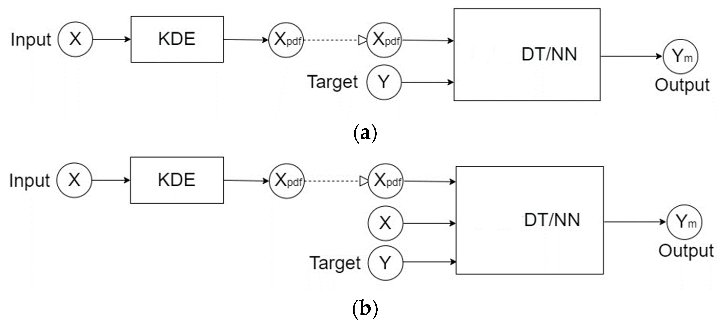
Figure 2.
The respective probability density functions estimated by KDE of case patients and control samples with the matching ratio of 1:1.
Figure 2.
The respective probability density functions estimated by KDE of case patients and control samples with the matching ratio of 1:1.
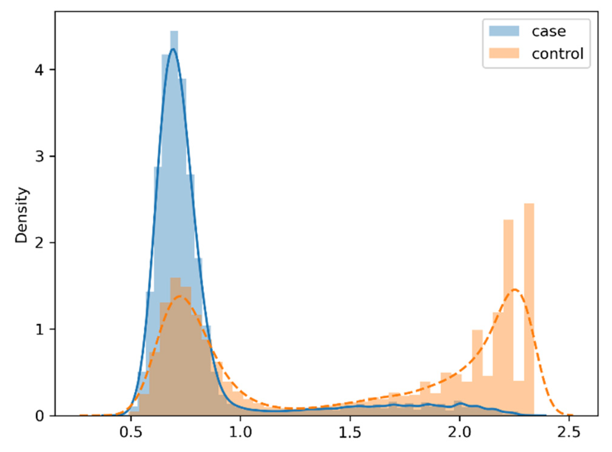
Figure 3.
The respective probability density functions estimated by KDE of case patients and control samples with the matching ratio of 1:3.
Figure 3.
The respective probability density functions estimated by KDE of case patients and control samples with the matching ratio of 1:3.
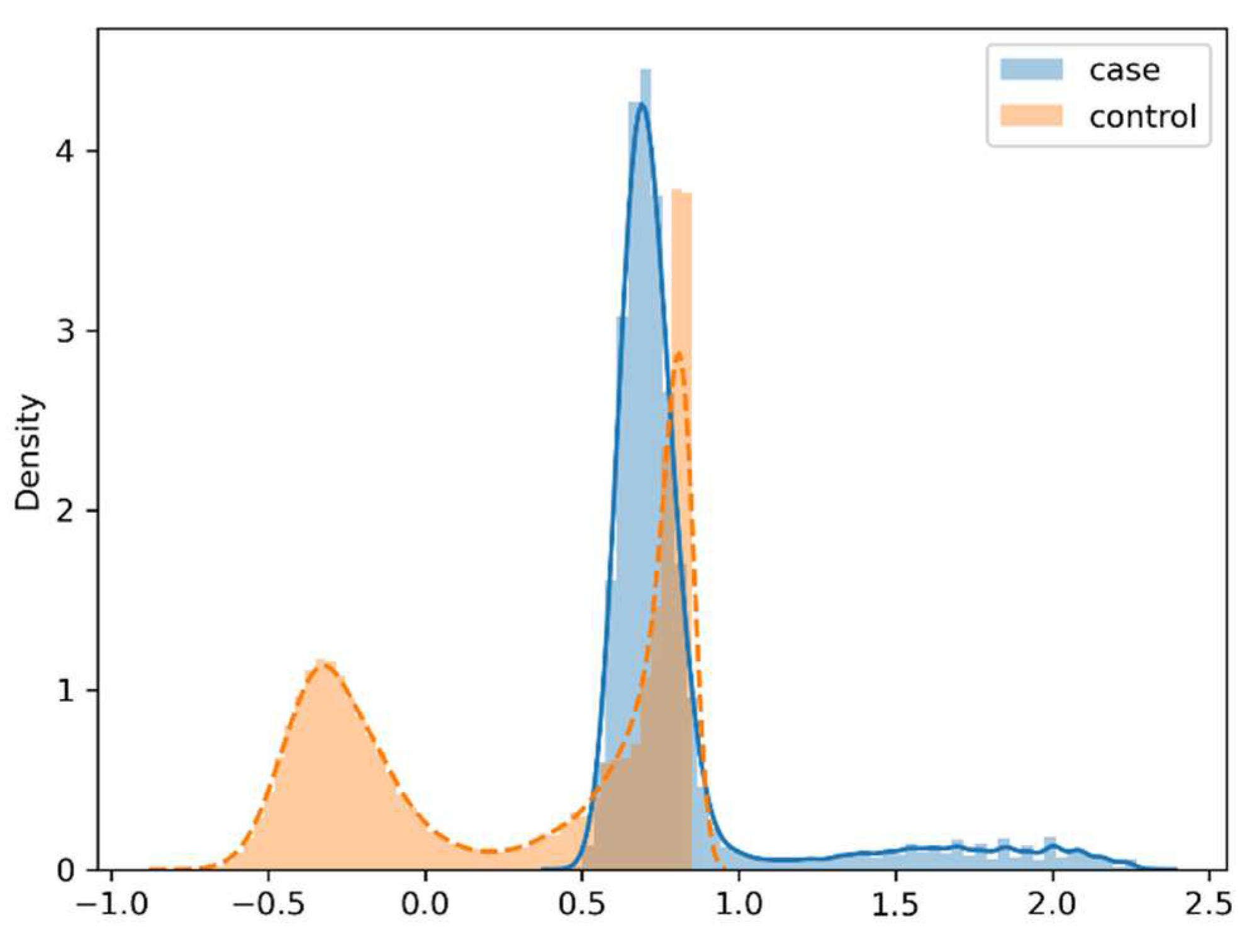

Table 1.
For cases and controls with the matching ratio of 1:1, the evaluation results of the testing set on prediction models of bipolar disorder trained using various learning algorithms. (a) Only use the soft label information Xpdf as the input attributes; (b) use both of X and Xpdf as the input attributes; (c) only use X as the input attributes.
| (a) | |||||||||
|---|---|---|---|---|---|---|---|---|---|
| The algorithm | TP | FP | TN | FN | Accuracy | PPV | NPV | TPR | TNR |
| Decision tree | 1371 | 561 | 1445 | 623 | 0.704 | 0.710 | 0.699 | 0.688 | 0.720 |
| NN(80, 10, 1) | 1597 | 500 | 1468 | 306 | 0.792 | 0.762 | 0.828 | 0.839 | 0.746 |
| NN(160, 40, 1) | 1551 | 549 | 1447 | 349 | 0.770 | 0.739 | 0.806 | 0.816 | 0.725 |
| NN(80, 20, 10, 1) | 1566 | 509 | 1489 | 358 | 0.779 | 0.755 | 0.806 | 0.814 | 0.745 |
| (b) | |||||||||
| The algorithm | TP | FP | TN | FN | Accuracy | PPV | NPV | TPR | TNR |
| Decision tree | 1579 | 425 | 1581 | 415 | 0.790 | 0.788 | 0.792 | 0.792 | 0.788 |
| NN(80, 10, 1) | 1602 | 482 | 1554 | 315 | 0.798 | 0.769 | 0.831 | 0.836 | 0.763 |
| NN(160, 40, 1) | 1620 | 389 | 1633 | 372 | 0.810 | 0.806 | 0.814 | 0.813 | 0.808 |
| NN(80, 20, 10, 1) | 1584 | 432 | 1563 | 401 | 0.791 | 0.786 | 0.796 | 0.798 | 0.783 |
| (c) | |||||||||
| The algorithm | TP | FP | TN | FN | Accuracy | PPV | NPV | TPR | TNR |
| Decision tree | 1563 | 425 | 1581 | 431 | 0.786 | 0.786 | 0.786 | 0.784 | 0.788 |
| NN(80, 10, 1) | 1549 | 483 | 1484 | 432 | 0.768 | 0.762 | 0.775 | 0.782 | 0.754 |
| NN(160, 40, 1) | 1612 | 444 | 1533 | 332 | 0.802 | 0.784 | 0.822 | 0.829 | 0.775 |
| NN(80, 20, 10, 1) | 1505 | 526 | 1449 | 464 | 0.749 | 0.741 | 0.757 | 0.764 | 0.734 |
Table 2.
For cases and controls with the matching ratio of 1:3, the evaluation results of the testing set on prediction models of bipolar disorder trained using various learning algorithms. (a) Only use the soft label information Xpdf as the input attributes; (b) use both of X and Xpdf as the input attributes; (c) only use X as the input attributes.
| (a) | |||||||||
|---|---|---|---|---|---|---|---|---|---|
| The algorithm | TP | FP | TN | FN | Accuracy | PPV | NPV | TPR | TNR |
| Decision tree | 979 | 1050 | 4945 | 1023 | 0.741 | 0.483 | 0.829 | 0.489 | 0.825 |
| NN(80, 10, 1) | 1363 | 991 | 5013 | 633 | 0.797 | 0.579 | 0.888 | 0.683 | 0.835 |
| NN(160, 40, 1) | 1307 | 909 | 5094 | 690 | 0.800 | 0.590 | 0.881 | 0.654 | 0.849 |
| NN(80, 20, 10, 1) | 1434 | 1041 | 4914 | 611 | 0.794 | 0.579 | 0.889 | 0.701 | 0.825 |
| (b) | |||||||||
| The algorithm | TP | FP | TN | FN | Accuracy | PPV | NPV | TPR | TNR |
| Decision tree | 1315 | 710 | 5285 | 690 | 0.825 | 0.649 | 0.885 | 0.656 | 0.882 |
| NN(80, 10, 1) | 1560 | 394 | 5588 | 458 | 0.894 | 0.798 | 0.924 | 0.773 | 0.934 |
| NN(160, 40, 1) | 1265 | 591 | 5410 | 734 | 0.834 | 0.682 | 0.881 | 0.633 | 0.902 |
| NN(80, 20, 10, 1) | 1278 | 717 | 5325 | 680 | 0.825 | 0.641 | 0.887 | 0.653 | 0.881 |
| (c) | |||||||||
| The algorithm | TP | FP | TN | FN | Accuracy | PPV | NPV | TPR | TNR |
| Decision tree | 1276 | 752 | 5243 | 729 | 0.815 | 0.629 | 0.878 | 0.636 | 0.875 |
| NN(80, 10, 1) | 1196 | 739 | 5238 | 827 | 0.804 | 0.618 | 0.864 | 0.591 | 0.876 |
| NN(160, 40, 1) | 1184 | 725 | 5260 | 831 | 0.806 | 0.620 | 0.864 | 0.588 | 0.879 |
| NN(80, 20, 10, 1) | 1179 | 788 | 5215 | 818 | 0.799 | 0.599 | 0.864 | 0.590 | 0.869 |
Disclaimer/Publisher’s Note: The statements, opinions and data contained in all publications are solely those of the individual author(s) and contributor(s) and not of MDPI and/or the editor(s). MDPI and/or the editor(s) disclaim responsibility for any injury to people or property resulting from any ideas, methods, instructions or products referred to in the content. |
© 2023 by the authors. Licensee MDPI, Basel, Switzerland. This article is an open access article distributed under the terms and conditions of the Creative Commons Attribution (CC BY) license (http://creativecommons.org/licenses/by/4.0/).
Copyright: This open access article is published under a Creative Commons CC BY 4.0 license, which permit the free download, distribution, and reuse, provided that the author and preprint are cited in any reuse.


