Preprint
Article

Performance of Lip-sync instead of Speech Imagery, New Combination Signals, Supplement Bond Graph Classifier and Deep Formula Detection as Confidents Extraction and Roots Detection Classifier for EEG and BCI

Altmetrics

Downloads

141

Views

67

Comments

0

A peer-reviewed article of this preprint also exists.

This version is not peer-reviewed

Submitted:

05 August 2023

Posted:

07 August 2023

You are already at the latest version

Alerts
Abstract
Nowadays, brain signal processing is performed rapidly in various brain-computer interface (BCI) applications. Most researchers focus on developing new methods for the future or improving the basic implemented models to identify the optimum standalone feature set. Our research focuses on four ideas. One of them introduces future communication models, and the others are for improving old models or methods. These are: 1) new communication imagery model instead of speech imager using the mental task: Due to speech imagery is very difficult, and it is impossible to imagine sound for all of the characters in all of the languages. Our research introduces a new mental task model for all languages that call Lip-sync imagery. This model can use for all characters in all languages. This paper implemented two lip-sync for two sounds, characters or letters. 2) New combination Signals: Selecting an inopportune frequency domain can lead to inefficient feature extraction. Therefore, domain selection is so important for processing. This combination of limited frequency ranges proposes a preliminary for creating Fragmentary Continuous frequency. For the first model, two s intervals of 4 Hz as filter banks were examined and tested. The primary purpose is to identify the combination of filter banks with 4Hz (scale of each filter bank) from the 4Hz to 40Hz frequency domain as new combination signals (8Hz) to obtain well and efficient features using increasing distinctive patterns and decreasing similar patterns of brain activities.3) new supplement bond graph classifier for SVM classifier: When SVM linear uses in very noisy, the performance is decreased. But we introduce a new bond graph linear classifier to supplement SVM linear in noisy data. 4) a deep formula recognition model: it converts the data of the first layer into a formula model (formula extraction model). The main goal is to reduce the noise in the subsequent layers for the coefficients of the formulas. The output of the last layer is the coefficients selected by different functions in different layers. Finally, the classifier extracts the root interval of the formulas, and the diagnosis does based on the root interval. For all of the ideas achieved the results of implementing methods. The results are between 55% to 98%. Less result is 55% for the deep detection formula, and the highest result is 98% for new combination signals.
Keywords: 
Subject: Engineering  -   Bioengineering

1. Introduction

Brain-Computer Interface (BCI) systems have been established to direct communication in the human brain and external environment [1,2,3,4,5]. These systems act as a communication channel for exchanging information and controlling external devices [5]. The BCI systems such as EEG can measure signals of movement imagination modulation of the brain’s electrical activities [6]. The origin of motor area neurons activation is real movement or imagination movement. These two movements are somewhat similar in motor area neurons activation [7]. Different measurable EEG patterns are discovered based on different kinds of motor imagery. Different EEG signals such as mu and beta rhythms show cortical potentials [8], event-related P300 [9,10], visual evoked potentials [11], and so on. Motor imagery (MI) is one of many kinds of BCIs systems used in most researches over the past decades. The Motor Imagery-BCI (MI-BCI) is suitable and safe for noninvasive measurement. The advantages of Motor Imagery include an advanced approach for signal processing and the least auxiliary equipment.
Preprocessing, feature extraction, and pattern classification of EEG signals are core parts of the BCI systems. EEG signals are consist of source brain signals and noise [12]. To simplify the problem, raw EEG signals can be considered linear. As an essential part, the preprocessing part acts for removing noise. The next part is feature extraction which is a very crucial part. One famous feature extraction approach for MI-BCI is Common Spatial Pattern (CSP) [4], [13], [14]. CSP includes an effective feature extraction approach and a popular spatial filtering algorithm for two MI tasks classification. For accurate classification, effective parameters are the best frequency band and the associated filter parameters. The optimum frequency band depends highly on users and measurement. Hence it is necessary to find the optimum frequency band for each user/ or dataset separately.
Many methods for solving the problem of finding the effective parameters, i.e., finding the best frequency band and the associated filter parameters have been proposed [15,16,17,18]. For using CSP for the combination of two different signals (observed with the time-delayed signals) following methods are introduced: 1) Common Spatial-Spectral Pattern (CSSP) [15] and 2) Common Sparse Spectral-Spatial Pattern (CSSSP) [16]. These approaches obtain coefficients of a Finite Impulse Response (FIR) filter. CSSP has a time delay drawback and a limitation. Hence, CSSP provides very poor frequency selectivity. Even having the time delay limitation CSSP can provide different spectral patterns for any channel. In comparison, CSSSP can provide different spectral patterns for all channels.
Computationally optimization of CSSSP is expensive and high. It requires a high cost and extensive parameter tuning optimization for filter parameters. In the methods of the spectrally weighted common spatial pattern (SPEC-CSP) [17] and iterative spatial-spectral patterns learning (ISSPL) [18] for optimizing filters and spatial weights, iterative procedures are used. Therefore, for the spectrum, spatial weights and filter parameters are optimized by CSP and weights, which could find them using some criteria. It could lead to solving the two optimization problems, i.e., finding the best frequency band and the associated filter parameters. Based on different cost functions, these two problems cannot guarantee that they will be converged.
In the paper [19], the sub-band common spatial pattern (SBCSP) is introduced, and the filter bank common spatial pattern (FBCSP) [20] is used on sub-band decomposition. The main idea of these approaches is to decompose the raw EEG signals into multiple frequency bands, which include different pass bands as filter banks. CSP has extracted the most discriminative features on each band, which leads to an increase in classification accuracy. However, this will seriously damage the raw signals when the EEG signals are decomposed to narrow overlapping frequency bands, leading to a drop in the classification accuracy. To avoid the decrease in the quality of EEG signals, it is necessary to decompose EEG signals into fewer parts in the form of suitable scale frequency bands, leading to less damage for EEG signals. Based on several studies, MI can cause an increase or decrease in frequency rhythms energy in the related cortical areas, which illustrates fixed frequency bands that contain the discriminative information.
In addition to the previously mentioned methods, some methods for solving these problems are also proposed, which could not solve the problem completely. In the paper [21], Luo et al. used 7Hz to 30Hz and 7Hz-120Hz frequency range with the same method for extracting features. They reported a 1% higher average accuracy in the 7Hz-120Hz than the 7Hz-30Hz frequency range. This proves that most information related to distinctive activity patterns like left and right hand are in the 7Hz to 30Hz frequency range. The paper [22] compared using a 7Hz-30Hz pass band filter and ten filter banks on four subjects. The filter banks method could increase the accuracy better than 7Hz-30Hz band pass filter. In the paper [23], Zheng Yang Chin et al. argued that selecting different features for different subjects from some filter banks is necessary to increase average accuracy. The paper [23] explained the percentage of selecting features from each filter bank, where the subjects are selected from two to four filter banks. Most subjects used two filter banks, and the selected filter banks for each subject are different. For example, selected features for subjects 1 are 33% from filter bank 3and 67% from filter bank 6.

1.1. Speech Imagery with Mental Task

Before speech imagery research [24], the essential part of the classification began in 2009. First, Charles S. Da Silva[25] and all the video lectures of the two English characters researched with a practical mode for relaxation. In the second stage, Lee Wang and et. al [26] formed their mental task with/without speech imagination. Some researchers implemented other ideas. But the main ones implemented. According to all research, five English characters (a, e, u, o, i) are possible for humans to create sounds in the brain. It is also difficult to imagine these vowels easily for more time. Each researcher considers only their language, such as English, Chinese, etc. It is impossible to imagine sound of other characters.
Our paper focuses on lip movement to understand lips that have recognized lip synchronization. It also uses language for speech. But it cannot see language while speaking. Our research started contacting the sync language. Our idea chose M and A with a lip-sync model. The accuracy of our results shows that this method can improve future communication.
Why is the current method the good or the alternative to previous methods?
Lip-sync method is simple and easy to imagine. The advantage of this method is: 1) It does not cause fatigue for a long time. 2) It is possible to imagine for all ages. 3) It can be used as a base for all languages. By imagining them in order, it is possible to use letters possible for all languages. It causes the removal of letters and sounds of any specific language. It can generally approve the use of all languages.

1.2. FilterBank and Common Models

Based on the Fourier series [27,28], each signal consists of many sine waves with different pulses, phases, and amplitudes. Therefore, brain activity signals include different pulses, phases, and amplitudes in large special ranges. The main brain activity formula is supported by large-scale frequency bands based on EEG systems. But based on researches[19,20], the formula of distinctive patterns between brain activates are distributions in the range of 4Hz-40Hz [23] for more than two activates and 8Hz-30Hz [21] for only two activates. When all frequency domains are used for processing [21], it is crucial to find the best feature extraction methods to discover these distinctive patterns of all frequency-domain for extracting features. The focus of most researchers [15,16,17,18] was on 8Hz-30Hz to detect the distinctions of the brain activates such as left hand and right hand. Based on researches[13,14], important distinctive patterns of the brain activates are within 4Hz-40Hz and 8Hz-30Hz domains. When the researchers consider a large frequency domain for processing, it is necessary to process the most similar and distinctive patterns, which leads to extract ineffective features. And when the researchers consider a suitable limited frequency domain [20,21], it decreases the similar patterns while keeping most of the distinctive patterns, which leads to extracting effective good features. Based on research [19,20], finding small and suitable frequency bands with important distinctive patterns is necessary for increasing high accuracy classification. Many studies [15,16,17,18,19,20,21,22,23] confirm that the most distinctive patterns are distributed in the different frequency domains. This article aims to find a near-optimal, locally optimal, or slightly optimal frequency domain to extract the most distinctive features. The frequency range can be small and limited frequency ranges in between 4 Hz and 40 Hz. A specific large frequency domain can necessarily arise from several small frequency domains as filter banks. For this purpose, it can suggest combinations (two, three, four, etc.) with various filter sizes of limited banks (0.1, 0.2, 0.5, ..., 4.). Because in some articles, 4 Hz filter banks were applied for processing, and they have shown better performance. As a preliminary work, we use a combination of two limited frequency domains as filter banks, which lead to the discovery of the most significant distinct patterns of brain activity signals for classification. The level of classification accuracy can express as a measure of the proportion of distinctive patterns in the newly combined signals. Therefore, the ultimate goal of this paper is to find the frequency bands with the different features associated with many brain activities. This paper is considered two combinations of two filter banks as two small frequency bands in this paper. In future research, the majority of models will examine the types of combinations and the sizes of the types of filter banks. It will be possible for us to find the optimal maximum or close to the optimal maximum.
This paper focuses on different combinations of pairs of 4Hz sized filter banks to extract better features set for recognizing users’ brain activities with high accuracy. In some research [20,21], 4Hz as a small frequency range for the filter bank is applied. The new combination of filter banks was analyzed by CSP and FBCSP (CSP with mutual information) for extracting and selecting features, respectively. Moreover, some new features are extracted by the Lagrangian polynomial coefficients (LPC) method. Finally, the impact of the new combination signals was investigated by Principal components analysis (PCA).

1.3. Deep Learning Methods

Due to the availability of large data sets, researchers use neural networks to find a cheap and suitable solution. That’s why they learn deep learning architecture. These innovations have led to an increase in deep learning applications in the past two decades. Effectively, deep learning shows very well performance in processing images [29], videos [30], speech [31], and text [32]. Because neural networks update their variables automatically, it does not require much prior knowledge of the dataset, which is very difficult to interpret even for experts in large datasets. In recent years, due to the collection and availability of large-scale EEG data, deep learning has been used to decode and classify EEG patterns, which usually have a low signal-to-noise ratio[33].
The paper [34] reported lower accuracy after examining various EEG features and neural network designs. Jiraiocharonsak et al. [34] tried three different combinations of calculated features. But found that even a mixture of PCE, CSA, and PSD features could not correct SAE deficiencies for this data set. Xu and Plataniotis [35] compared the accuracy between SAE and several DBNs and found that DBNs with three restricted Boltzmann devices have different RBMs than SAE and DBN. Correlation layers use in five of these studies. Two of these five architectures were combinations that the CNN sends to the LSTM modules of the RNN, but none of these violate enough accuracy. The difference in accuracy in the three standard CNN studies is likely due to differences in the input formulation. Yanagimoto and Sugimoto [36] used signal values as input to the neural network, while [37,38] instead transformed the data into Fourier feature maps and 3D neural networks, and the accuracy is excellent. These CNN architectures consist of two convolutional layers, each with one or two dense layers. Only the MLPNN architecture applied to this dataset [36] achieved very well accuracy, comparable to the standard CNN that uses signal values. But the input formulation may be the main factor in the difference in accuracy. While CNN Deep uses signal quantities that require significant preprocessing, MLPNN requires extensive effort to preprocess the input with PSD features and forward asymmetry channel selection.
First, architecture includes two layers of LSTM [39] with one dense layer, which consider for an RNN network. The networks without convolution layers create. For the higher cases of this group, a deep learning regression architecture without convolution layers built to outperform other architectures look like iterative and motion aspect architectures. With the investigations done for that dataset, DBN, CNN, and RNN architectures are known as the most suitable and effective architectures. The selection of good formulas made the input suitable for CNN. Signal values for RNN, while computed properties, especially PSD properties, work better for DBN.
Machine learning provides and applies models as an effective solution [40,41,42,43] for most cases, because neuroscientists provide knowledge and procedures for processing and diagnosis, all cases of signal variability over time and led by machine learning approaches. Many classifiers such as neural networks [44,45,46,47,48,49], support vector machines (SVM) [50], [51] and hidden Markov models [52], [53] have been used to classify EEG signals. Detection of mental activity patterns based on potentials by updating neural networks with a propagation approach after EEG classification are used [54]. Researchers have used deep learning based on neural networks (CNN, RNN, etc.) to solve complex problems, and have made them perform very well in these fields [55,56,57,58,59,60,61,62,63,64,65,66,67,68,69].
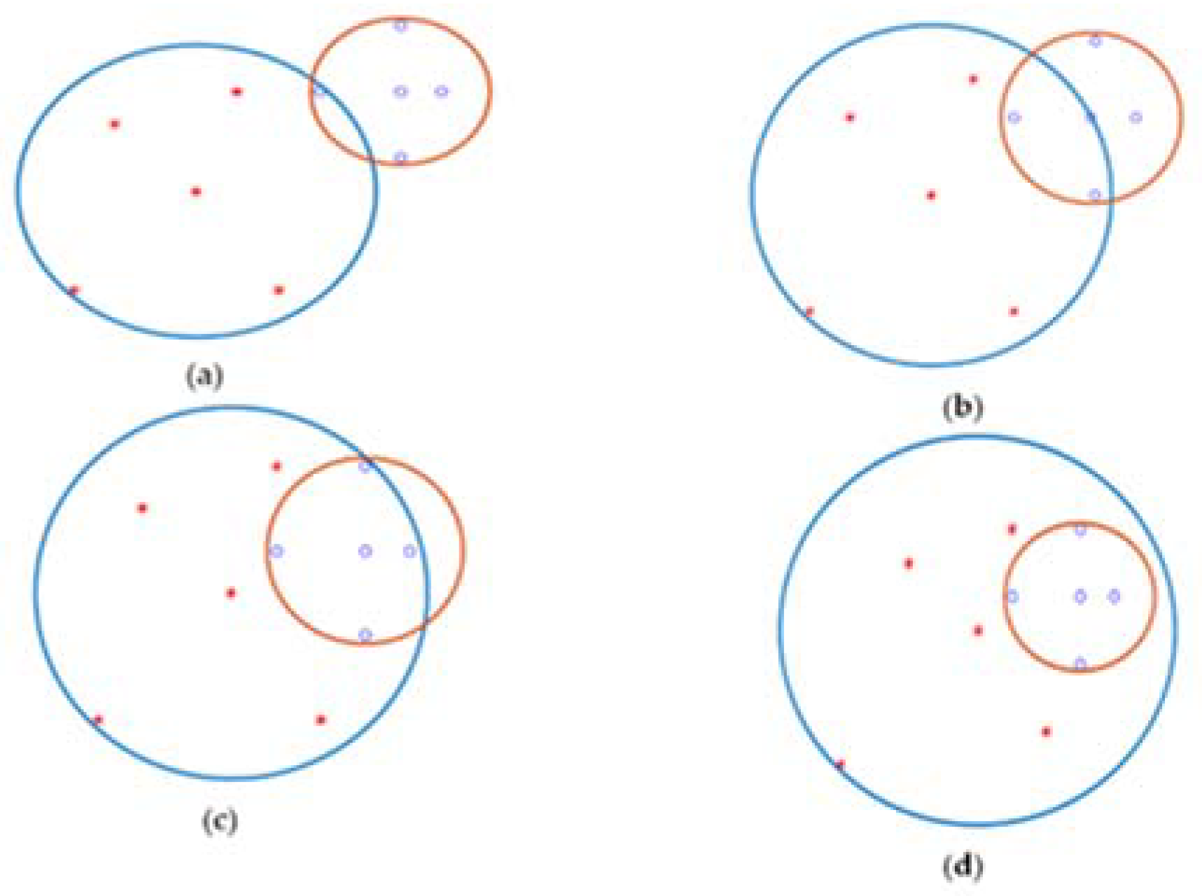
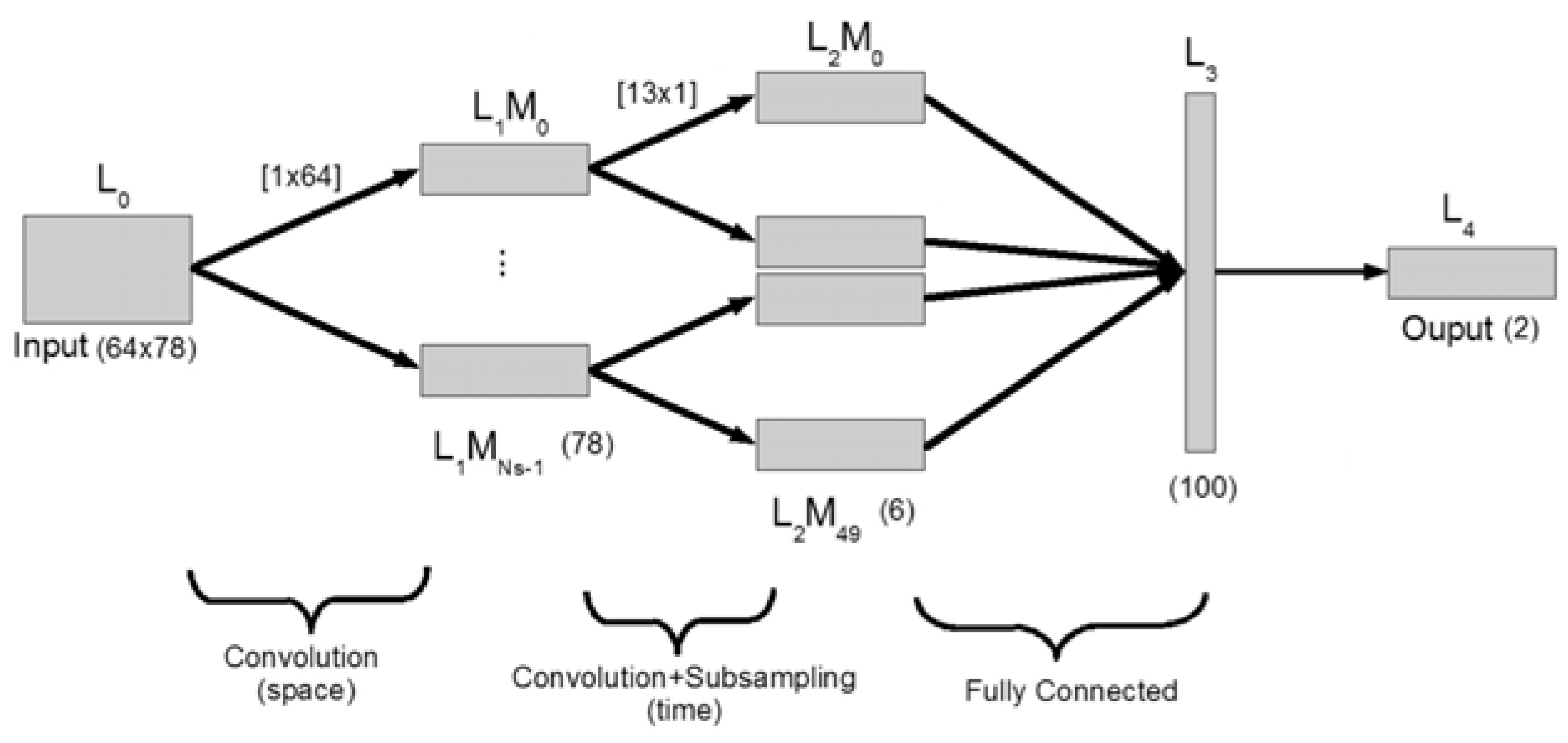
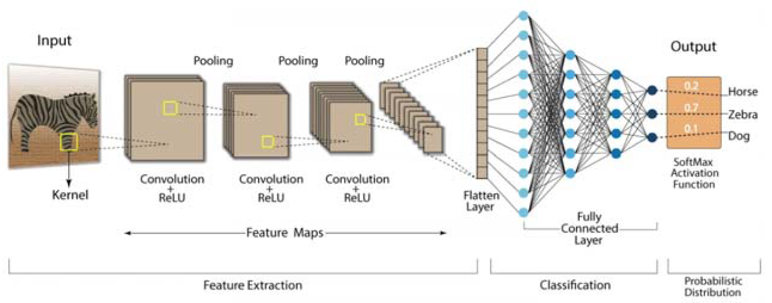
In [70], the authors propose a new form of feature that preserves the spatial, spectral, and temporal structure of the EEG. In this method, the signal power spectrum of each electrode is estimated, and the sum of absolute square values is calculated for three selected frequency bands. Then, the polar drawing method is used to map the electrode locations from 3D to 2D and creates input images (Figure 1 and Figure 2).
This article proposed to present one idea related to deep learning, which can achieve significant success by improving them because deep learning structure depends on proper designs of neural networks, which have a worthy effect on network structure. Our ideas are, respectively:
Extraction and selection of formulas related to brain activities along with finding the root of the formula related to brain activities: first, based on the data input, the input data convert into a formula (the first layer converts the characteristic layer of the data into equation coefficients based on the Lagrange formula In our model, this transformation is chosen based on the window size to extract the coefficient of Eq. In the subsequent steps (network layers), some coefficients are selected based on the definition of specified functions (the second layer selects some of these formulas based on the integration of the sampling model). The coefficients that have an excellent effect on the difference between the activities, then well results can achieve. We considered the first evaluation selection model. It is a simple function that selects the high value of the high-order transaction coefficient. Therefore, the output of the last layer for classification is a combination of coefficients of different activity formulas. Our proposed classification is root classification, which has three stages. A) The first part extracts all the intervals of the roots of each vector (combination formula). b) Finding the interval of the roots of each class based on the training formula (such as training data) c) The test recognition formula (such as the test data) based on the intervals of the roots of each class: a formula belongs to the class that has the maximum similarity to the intervals are the roots of that class. In the following, prevalent and general classifiers are also used to classify the body of the root class clause.
Ideas achieved different results. Some are minimum results of 55% and maximum results of 98%. Some ideas achieved good results, and some had middle and some weak results. Weak results can improve with a few changes in parts of some ideas.
This article is organized as follows; In section 2, proposed methods are presented. In the third section, experiments and results are presented. In section 4, the results are analyzed and compared with the previous similar methods. Finally, the concluding remarks and recommendations for future work are provided in section 5.

2. Proposed Methodology

2.1. Speech Imagery Based on Mental Task

Before speech imagery research [24], the essential part of the classification began in 2009. First, Charles S. Da Silva[25] and all the video lectures of the two English characters researched with a practical mode for relaxation. In the second stage, Lee Wang and et. al [26] formed their mental task with/without speech imagination. Some researchers implemented other ideas. But the main ones implemented. According to all research, five English characters (a, e, u, o, i) are possible for humans to create sounds in the brain. It is also difficult to imagine these vowels easily for more time. Each researcher considers only their language, such as English, Chinese, etc. It is impossible to imagine sound of other characters.

2.1.1. Speech Imagery Based on Lip-Sync

Our electrode cap has 32 channels related to the 10-20 international system. It is placed on the head to record EEG signals. The electrodes are distributed in different parts of the brain.
It is difficult for volunteers to imagine all the lips. Our research only considered the lip border as a line in 2D and a page in 3D to synchronize the language because it is easy to imagine and learn for all ages. The performance of these ideas depends on learning. This model is like the language of deaf people for all languages. Development this model for all sounds creates a new model for future communication. Our paper focuses on analyzing and classifying EEG signals from a mental task related to lip synchronization. The EEG signals collected the M and A sounds by lip synchronization with three Chinese volunteer students. Educated people are in good health.
Based on this idea, our model wants to create another idea for the communication person look like visual communication. This new idea uses lips and language synchronization. It can also be created based on one of them. But it is difficult for us to get a good result for it. Our model should make about 30 to 40 sounds for our area. First, it used a combination of them for this area with two basic sounds.
Lip synchronization is one way that some people can understand. Learning for any person is hard. Some articles have a formula for it.
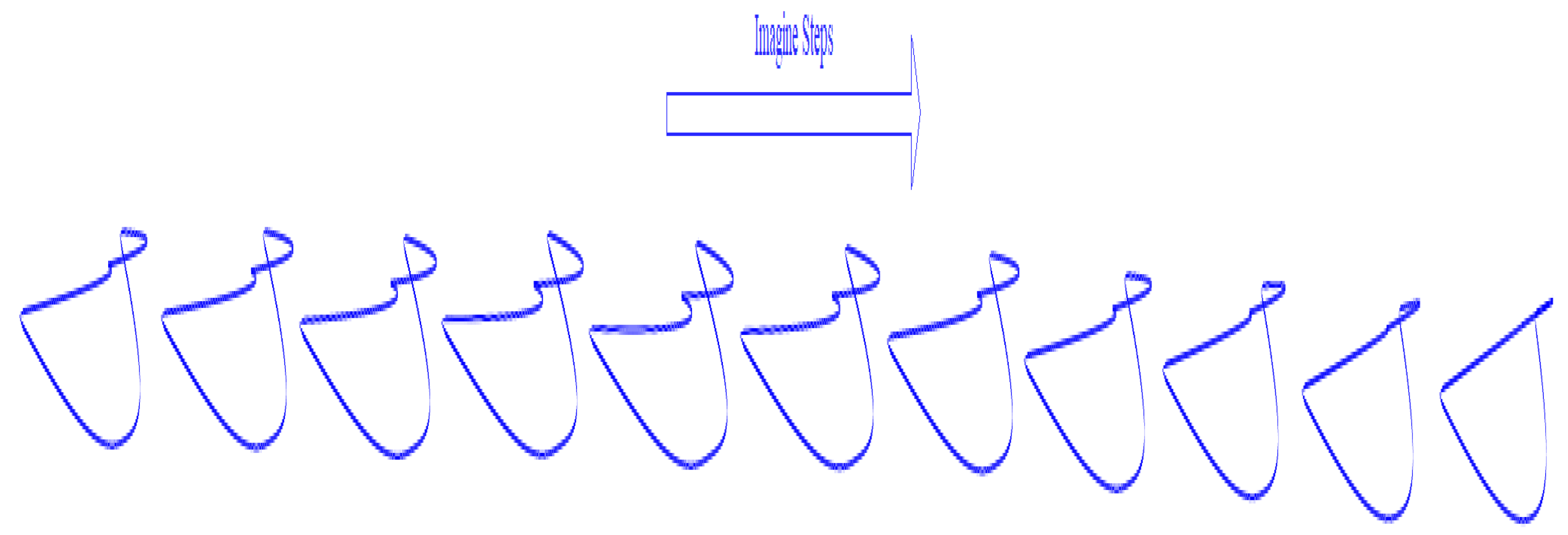
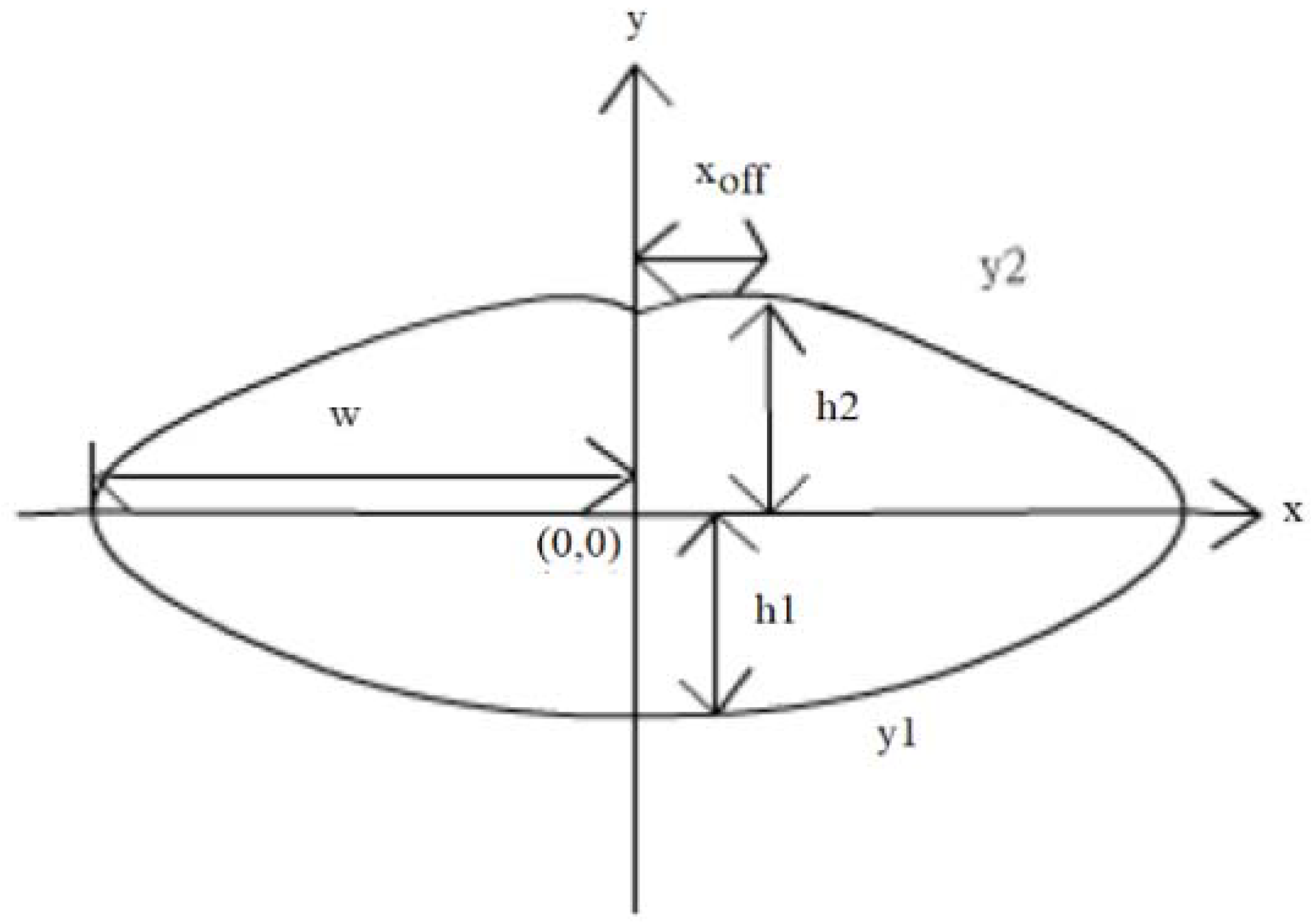
The lip-sync [71,72,73,74,75,76,77,78,79] contour formula is one of these formulas for detecting lip movement. Our model uses a lip liner for two created sounds. Figure 3, Figure 4 and Figure 5 show the steps of a sound based on lip and contour synchronization. Lip imagination is two-dimensional (2D) or three-dimensional (3D).
The formula of the contour of the lip is
y 1 = h 1 ( ( x sy 1 w ) ) 1 + σ 2 h 1
y 1 = h 2 ( w x eff ) 2 ( | x sy 2 | x eff ) 2 + h 2
H1 is the height of the lower lip, and H2 is the height of the upper lip. w is half of the mouth width. Xeff is the amount of curvature or the middle curve on the upper lip.

2.1.2. Signal Collection Datasets

Three Xian Jiaotong University volunteers collaborate with our experiment in a non-feedback the experiment. Their age is 30-40 years, the average age is about thirty five years old, and the standard deviation is three years. Our volunteer was in good health. They trained to work mentally with their lips and synchronize their language using video. The experiment is conducted under a test protocol under Xi’an Jiaotong University. All volunteers sign informed consent to the test. It explained for volunteers how to think and other details. People sit in a comfortable chair in a lab, about 1 meter in front of a 14-inch LCD monitor.

2.1.3. Filter in frequency Domain

Our electrode cap has 32 channels related to the 10-20 international system. It is placed on the head to record EEG signals. Based on some researches distributed electrodes in different brain parts such as the Broca and Wernicke area, the superior parietal lobe, and the primary motor area (M1). SynAmps system 2 EEG signals recorded. Vertical and horizontal electrooculogram (EOG) signals are recorded by two bipolar channels to control eye movements and blinking. EEG signals are recorded after passing through the 0.1 to 100 Hz bandwidth filter, and the sampling frequency set to 256 Hz. The skin impedance is also maintained below 5   k Ω .

2.1.4. Independent component analysis (ICA)

Independent component analysis (ICA) is a very broad method for EEG signal preprocessing. This is a classic and efficient way to isolate the blind source, the first solution to the problem of cocktail parties. As researchers all know, similar to a cocktail party scene generally includes music, conversation, and unrelated types of noise. Although scene is very messy because the person himself can see someone with the content He speaks and hears, the man forces himself to identify himself and wants to instinct content of the signal source, but this scene is deadly of various kinds. Blind and sources signals mix to make target source signal cocktail effect. Independent component analysis algorithm proposed for that purpose and allows the computer to have the ability to complete the same ear of interest. Component-independent component analysis algorithms assume that each source component is statistically independent.

2.1.5. Common Spatial Pattern (CSP)

Koles and eta have introduced a Common Spatial Pattern (CSP) that can detect abnormal EEG activity. CSP tries to find the maximum discrimination between different classes by using signal conversion to variance matrix. EEG pattern detection performs using spatial information extracted with a space filter. CSP only requires more electrodes to operate and does not require specific frequency bands and knowledge of these bands. CSP is also very sensitive to the position of electrodes and artifacts. The same electrode positions in the training process are related to memorization to collect similar signals. It is effective for increasing accuracy as obsolete.

2.2. New Combination Signal Model with Four CommonMethods

Most researchers [15,16,17,18,80] have used a large-scale frequency domain consisting of known brain activities and some noise representing unknown brain activities. A large-scale frequency filter could divide into overlapping narrow frequency filters to extract high discriminate features [19,20]. The disadvantage of decomposing the EEG signal into narrow-pass filters is the damage to the raw EEG signals. The essential information of each distribution event is in a large frequency band. The damage is related to removing more EEG frequency range for processing. The main EEG signals of the events are lost. The main goal of the model is to find the most important patterns of different events in small frequency bands and to find more frequency ranges of more similar patterns. Choosing an appropriate scale for frequency filters is essential to avoid damage to raw EEG signals and to reduce noise in EEG signals. Our model is reduced damage. For collecting important distinctive patterns of brain activities, it is necessary to combine several essential small-scale frequency bands for classification. The combination of two fixed filter banks introduces new combination signals. These models investigate three feature extraction methods and one feature selection method.
To the best of our knowledge, at the time of writing this paper, using the combination of two fixed filter banks with a 4Hz domain (limited frequency bands) is used for the first time with this scale in this paper. This leads to creating new combination signals with 8Hz domains in total. The accuracy performance of new signals has been studied by two feature extraction methods, i.e., CSP, FBCSP, and one feature selection, i.e., PCA. In addition to three common methods, a lagrangian polynomial equation is introduced to convert data structure to formula structure for classification. The purpose of the lagrangian polynomial is to detect important coefficients for increasing a distinction of brain activities. It may be noted that the concept of the lagrangian polynomial is different from Auto-regression (AR), in which features are coefficients for classification.
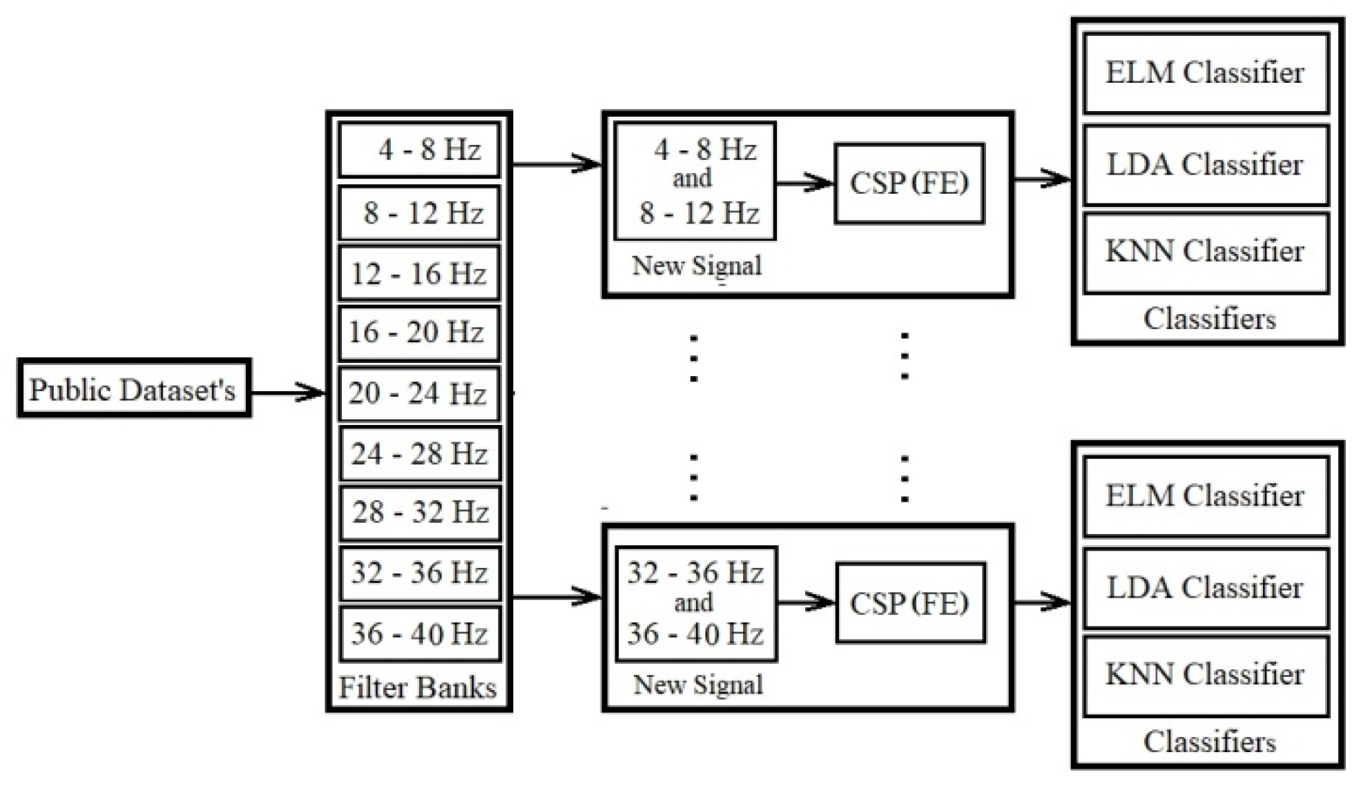
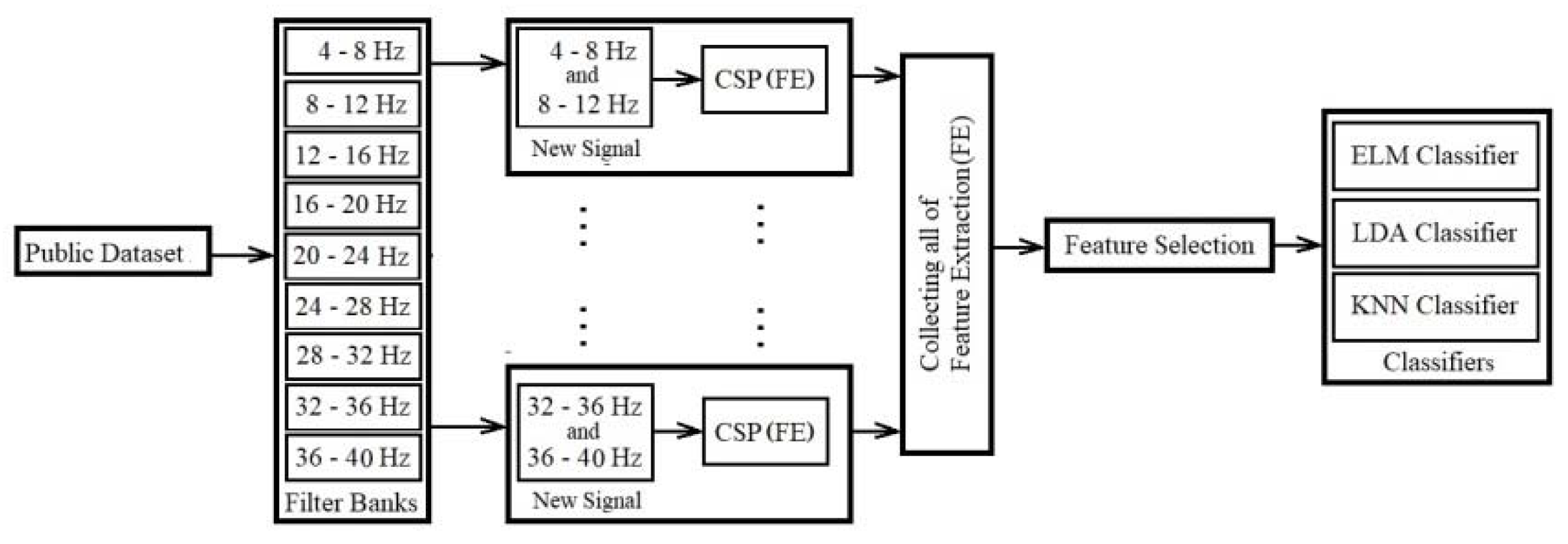
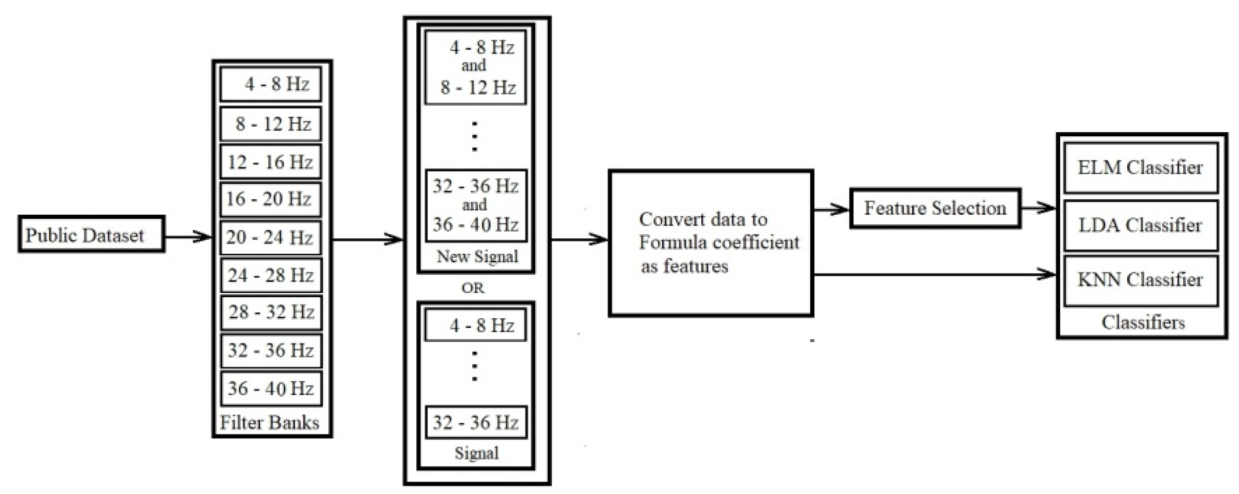
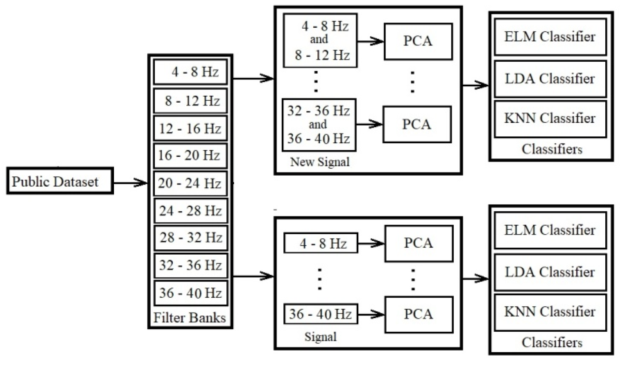
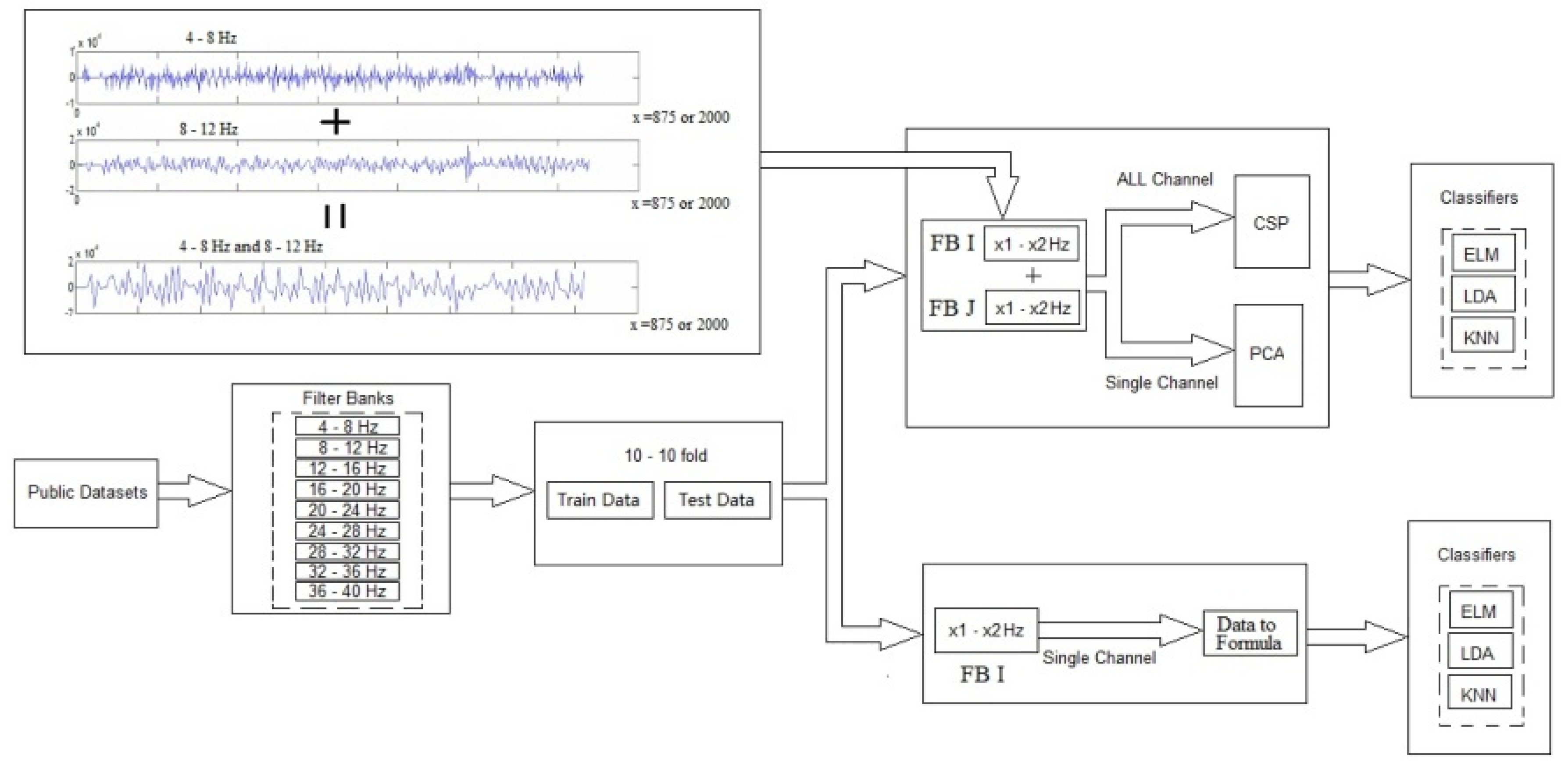
In the following subsections, we explain the details of the four main contributions of this paper by describing the models. We show an overview of four implemented models in Figure 1, Figure 2, Figure 3 and Figure 4. Figure 5 provides an overview of the database, filter banks, and the model of the new combination signals with the classifiers.

2.2.1. CSP Using New Combination Signal

The first proposed model increases the extracted good distinctive features on the whole channel. In this model new combinational signals are created and applied individually in the classification. In this case, all of the electrodes are involved in extracting features. The model consists of four phases as presented in Figure 6 and explained below:
1) Filtering data by Butterworth filter: In the first phase, using frequency filtering, noises and artifacts are removed with a filter bank. The domain of these filter banks is out of the noise and artifact domain. EEG measurements are decomposed into nine filter banks from 4-8Hz, 8-12Hz, …,36-40Hz. All of the data using the Butterworth filter is filtered by 100th order. Most of researcher use the Butterworth filter for filtering [20,21].
2) Creating new combination signals: The combination of the two fixed filter banks creates new combination signals. Each fixed filter bank has a 4-frequency range. For example, filter bank 5 starts with 20Hz (lower band) and ends with 24Hz (upper band). The new combination signal of filter banks 2 and 5 support the 8Hz to 12Hz and the 20Hz to 24Hz frequency ranges.
The formula of new signals for all of the electrodes is calculated as:
FB ( i , j , m ) = FB ( i , m ) + FB ( j , m ) .   i ,   j = 1 9 , ,   m = 1 n .
where FB(i,j,m) represents the ith and jth Filter bank of mth channel and n is the maximum electrodes of a dataset that data is recorded. Therefore, m and i variables indicate the selected channel and selected 4Hz-ranged domain frequency(for example, m=2 and i = 2, means channel 2 and 8Hz-12Hz frequency range).
3) Using CSP as the spatial filter and feature extraction: The common spatial pattern algorithm [81,82,83,84] is known as an efficient and effective EEG signal class analyzer. CSP is a feature extraction method that uses signals from several channels to maximizes the difference between classes and minimizes their similarities. This is accomplished by maximizing the variance of one class by minimizing the variance of another class.
The CSP calculation is done as follows
C = E   E   / trace ( E   E   )  
where C is the covariance of the normalized space of data input E, which provides raw data from a single imaging period. E is a N×T matrix where T is the number of electrodes or channels, and N is the number of samples in the channel. The apostrophe represents the transposition operator. Trace is also a set of diagonal elements of x.
The covariance matrix of both classes C1 and C2 is calculated by the average of several imaging periods of the EEG data, and the covariance of the combined space Cc is calculated as follows:
C c = C 1 + C 2
C c is real and symmetric and can be defined as follows:
C c = u c λ c u c
where u c is a matrix of eigenvectors and λ c is the diameter of the eigenvalues matrix.
p = λ 1 u c  
The variances in space are equalized by u c and all eigenvalues of p c ¯ L   p   are set to 1.
S L = p c ¯ L   p  
S R = p c ¯ R   p  
S L and S R are common special sharers, provided that S L = B λ L   B   and S R = B λ R   B   and λ L + λ R = I .
Eigenvalues are arranged in descending order. And the projection matrix W is defined as follows:
W = U T P  
where U T and P are transfer matrix and data.
The reflection matrix of each training is as follows
Z = W × i
where N rows are selected to represent each period of conception W P ( p = 1 , 2 , , N ) and the covariance P of Z , P components of the feature vectors are calculated for the nth instruction.
Normalized variance used in the algorithm is as follows:
f p = log 10 ( Var ( Z p ) / Var ( Z p ) )
4) Classification by Classifiers: Classification is done using three classifiers in our model, including LDA with a linear model, ELM with the sigmoid function using 20 nodes, and KNN with five neighborhoods (k=5).
Two public datasets are selected according to details described in next Section. After filtering data, the combinations of two filter banks based on formula (1) for all of the electrodes are created. Each combination of two filter banks is considered separately for the next steps. In the next step, CSP is applied for spatial filtering, removing artifacts, and extracting features on the new combination signal. The experimental model of train data and test data is presented in section 3.

2.2.2. FBCSP[85,86,87] Using New Combination Signal

The second proposed model increases the good extracted distinctive features on the whole channel, which have the additional step of feature selection to the first model. In this model new combination signals are created, and the best signals from both primary and new signals are selected using the feature selection and used the classification. All of the electrodes cooperate for noise and artifact filtering and extraction of features. This model consists of the following phases presented in Figure 7 and explained below:
1) Filtering data by Butterworth filter: This step is the same as the first step in the previous section, i.e., 2.2.1.1.
2) Creating new combination signals: This step is the same as the second step in the previous section, i.e., 2.2.1.1.
3) CSP as the spatial filter and feature extraction: In this phase, the CSP algorithm extracts m pairs of CSP features from new combination signals. This is performed through spatial filtering by linearly transforming the EEG data. Then features of all new signals are collected in a feature vector for ith trial, i.e.:
X i = [ cf 1 , cf 2 , , cf 9 ]
where cf b 2 m denotes the m pairs of CSP features for the b th band-pass filtered EEG measurements, X i   1 × ( 9 * 2 m ) .
4) Features collection and selection: In this phase, an algorithm called Mutual Information Best Individual Features (MIBIF) is used as feature selection from the extracted features, and it selects the best features that are sorted (descending order) using class labels.
In general, the purpose of the mutual information index in MIBIF [88,89] is to obtain maximum accuracy k features are selected that from a subset of S F ,   which the primary set F includes d features. This approach maximizes the mutual information I(S; Ω). In the classification of features, input features, i.e., X, are usually continuous variables, and the Omega class (Ω) has discrete values. So the mutual information between the input features X and class Ω is calculated as:
I ( X ; Ω ) = H ( Ω ) H ( Y | Ω )  
Where   ω   Ω   = { 1 , .. ,   N ω }
And the conditional entropy is calculated as:
H ( Ω | X ) = X ω = 1 N ω p ( ω | X ) log 2 p ( ω | X ) dx ,
Where the number of classes is Nω.
In general, there are two types of feature extraction approaches in mutual information technique, including wrapper and filter approach.
With a wrapper feature selection approach, conditional entropy simply is in the in (14):
H ( Ω | X ) = ω = 1 N ω p ( ω | X ) log 2 p ( ω | X ) ,
P(ω|X) can be estimated easily from the data samples that are classified as class ω using the classifier over the total sample set.
Mutual information based on the filter approach is described briefly in three steps:
Step1: Initialization of set d feature F = { f 1 , f 2 , , f d } , and selected features set S=Null.
Step2: Compute MI features based on I( f i |Ω) for each i=1…d, and f i belong to F
Step3: Select k best features that maximize I( f i |Ω) [87,88]
Step4: Repeat the previous steps until | S | = k .
5) Classification by Classifiers: This step is the same as the fourth step in the previous section, i.e., 2.2.1.1.
This model is applied to one public dataset (including left hand and right hand), which is described in next section. Most of the steps in the two models are the same. Except, one phase as feature selection is added between CSP and classifiers, which selects the best features by mutual information feature selection after collecting the extracting features of new combination signals. Selected features are about 10 to 100 features, which are sent to classifiers for classification.

2.2.3. Lagrangian Polynomial Equation Using New Combination Signal

The third proposed model increases the good extracted distinctive features on every single channel separately. In this model, we a Lagrangian polynomial model for transforming the data into formulas that are then used as features in classifications. A single channel/electrode cooperates for extracting features and classification, as illustrated in Figure 8 and explained in the following steps.
1) Filtering data by Butterworth filter: In the first phase using frequency filtering, the noises and artifacts are removed with a filter bank. This process is the same as the first step in section 2.2.1.1, with the difference that it involves single channels individually
2) Filter banks (sub-bands) signals or new combination signals: Two models are considered as input data, including sub-bands in the name of filter banks and new combination signals. New combination signals are created based on the following formula for a single electrode. ​This formula is used for the calculation of a single electrode or channel.
S _ FB ( i , j ) = S _ FB ( i ) + S _ FB ( j ) .   i ,   j = 1 9.
where S _ FB ( i , j ) represents the filter bank signal.
3) Convert data to the formula of coefficients with different order by the Lagrangian polynomial equation: The input data is about one second from 3.5 seconds imagination time. Lagrangian polynomial equation converts these input data of the two single channels to coefficients for classification.
Lagrangian polynomial is described as:
There is k + 1 data asset ( x 0 , y 0 ) , , ( x j , y j ) , , ( x k , y k ) , while each x j is unique. The interpolation polynomial as a linear combination is in the Lagrange [86,87] form.
L ( x ) = j = 0 k y j j ( x )
The structure of Lagrangian polynomial is described in the form of:
j ( x ) = 0 m k x x m x j x m = ( x x 0 ) ( x j x 0 ) ( x x j 1 ) ( x j x j 1 ) ( x x j + 1 ) ( x j x j + 1 ) ( x x k ) ( x j x k )
where 0 j k . In fact, in the initial assumption, two x j aren’t the same, then (when m j ) x j x m 0 , therefore, this phrase is the appropriate definition. The reason pairs x i = x j with y i y j are not allowed, so no interpolation function L such that y i = L ( x i ) would exist, and the function gives unique value for each argument x i . On the other hand, if also y i = y j , therefore x i = x j are the same value as one single point. For all i j , i ( x ) includes the term ( x x i ) in the numerator, so that with x = x i the whole product will be zero, i ( x ) is:
( j i ) : j ( x i ) = m j x i x m x j x m = ( x i x 0 ) ( x j x 0 ) ( x i x 1 ) ( x j x 1 ) ( x i x k ) ( x j x k ) = 0
On the other hand
j ( x i ) = m j x i x m x j x m = 1
In other words, lagrangian polynomials are j ( x i ) = 0 at x = x i Unlessit is j ( x i ) = 1 as lack of the ( x x j = 0 ) term. It follows that y j j ( x i ) = y j , so at each point x j , L ( x j ) = y j + 0 + 0 + + 0 = y j , shows that L interpolates the function entirely.
The final formula is:
( x ) = a n x n + a n 1 x n 1 + + a 1 x + a
where a n , a n 1 ,…, a 1 , a are coefficients of the Lagrangian polynomial, and n, n-1, n-2, …, 1 are the orders.
4) With/without feature selection methods: First, all features are used for the classification. Second, the best equation coefficients using the feature selection are selected for the classification.
5) Classification by Classifiers: In this phase, we perform classifications on features to determine accuracy using classifiers. This phase is similar to the last phase of the two above models.
This model is examined on one public dataset (including left and right hand) for examination. We describe this public dataset in more detail in next section. Single channels are applied for processing. Then the combination of two filter banks based on formula (17) for single electrodes/channels is calculated. Each combination is considered separately for the next steps. In the next step, two procedures are considered for processing. The first procedure uses fixed filter banks of a single channel, and the second procedure uses the new combination signals of a single channel. Then each procedure uses the lagrangian polynomial equation for converting data to formula structures. The lagrangian coefficients are considered as features for the classification. The feature selection is not used in the first procedure, but it is used in the second procedure. Mutual information feature selection selects the best features from 1 to 30 features. And finally, the selected coefficients as most effective features are sent to LDA, KNN, and ELM classifiers for classification.

2.2.4. PCA Using New Combination Signal

The fourth proposed model increases the good extracted distinctive features separately single-channels. In this model using PCA, we sort the data without dimensional reduction based on the best features before the classification. A single electrode cooperates for sorting the features and transforming to a new space followed by the classification as illustrated in Figure 9 and explained in the following steps:
Filtering data by Butterworth filter: The first phase is the same as the first phase of the previous model.
Filter banks (sub-bands) signals or new combination signals: The second phase is the same as the second phase of the previous model.
Sorting features by PCA: The purpose of PCA as an orthogonal linear transformation is to reduce the dimension by transferring data to a new space and sorting them. The greatest variance lies on the first coordinate as the first principal component and the second greatest variance as the second coordinate, and so on. PCA is introduced as one method for reducing primary features using the transformation of data to new space artificially [88,89,90,91].
The basic description of the PCA approach is as follows. Let’s define a data matrix X ( M × N ) where M is the number of observations and N is the number of features. Then C ( N × N ) is defined as the covariance matrix of matrix X :
C = [ Var ( X 1 ) Cov ( X 1 , X 2 ) Cov ( X 1 , X N ) Cov ( X 2 , X 1 ) Var ( X 2 ) Cov ( X 2 , X N ) Cov ( X N , X 1 ) Cov ( X N , X 2 ) Var ( X N ) ]  
Where: Cov ( X i , X j ) = 1 M 1 M ( X i ( k ) X ¯ i ) ( X j ( k ) X ¯ j ) and var ( X i ) = σ X i 2 .
Eigenvectors and eigenvalues matrix are produced by matrix C as:
Γ = Λ Γ = Γ Λ   Γ  
Where Λ ( N × N ) is a matrix of sorted eigenvalue ( λ 1 λ 2 λ N ) :
Λ = [ λ 1 0 0 0 λ 2 0 0 0 λ N ]
And Γ ( N × N ) is a matrix of eigenvectors (each column corresponds to one eigenvalue from matrix Λ ):
Γ = [ γ 11 γ 12 γ 1 N γ 21 γ 22 γ 2 N γ N 1 γ N 2 γ NN ]
Finally, the matrix of principal components is defined as:
Y = Χ Γ = [ y 11 y 12 y 1 N y 21 y 22 y 2 N y N 1 y N 2 y NN ]
Each of N features x 1 , x 2 , , x n can be explained with parameters from matrix Y as a linear combination of K first principal components: x mn = k = 1 K γ nk y nk .
Classification by Classifiers: The fourth phase is the same as the fourth phase of the previous model, with differences in the scale of input data.
This model uses the entire 3.5 seconds as input with the PCA method. PCA is used for transferring data and sorting in our research.
Finally, we present the combination of filter banks in Figure 10.

2.3. New Linear and Nonlinear Bond Graph Classifier

The bond graph classifier uses a distance calculation method for classification. This model is local and focuses on the structure. Boundary uses point data centrally. Our model has different steps: 1) Search for the minimum path of nodes (attributes). 2) Create the center of the arc with the node and the longest sub-nodes. 3) Calculate the boundary between the two centers. 5) Create the main structure to support all borders. In this section, this paper begins with a brief description of the new classifier model in the main structure. Our idea explains in the following.
Our idea uses one of the greedy algorithms (Prim algorithm) to find the least spanning tree, which is weighted based on a directionless diagram. A subset of edges provides by the Prim algorithm to minimize the total weight of all tree edges. The algorithm arbitrarily starts the tree from one vertex to the vertex once. Then it adds the cheapest possible connection from the tree to the other vertex. Following the development of the algorithm in 1930 by the Czech mathematician Vojtěch Jarník, the algorithm was republished by computer scientists Robert C. Prim in 1957 and Edsger W. Dijkstra in 1959. These algorithms find at least a spanning diagram in a potentially truncated router. The most basic form of the Prim algorithm finds only minimal spanning trees in connected diagrams. In terms of asymptotic time complexity, these three algorithms are equally fast but slower than more complex algorithms. However, for graphs that are dense enough, the Prim algorithm can run in linear time, meeting or improving time limits for other algorithms. [92,93,94,95,96] (Figure 11).
This tree matrix has some nodes above and below the nodes. Each head node finds the smallest distance from its sub-nodes. They then create a slightly larger arc than the longest (27).
Distance_Arc = longest sub-nodes + alpha * longest subnodes
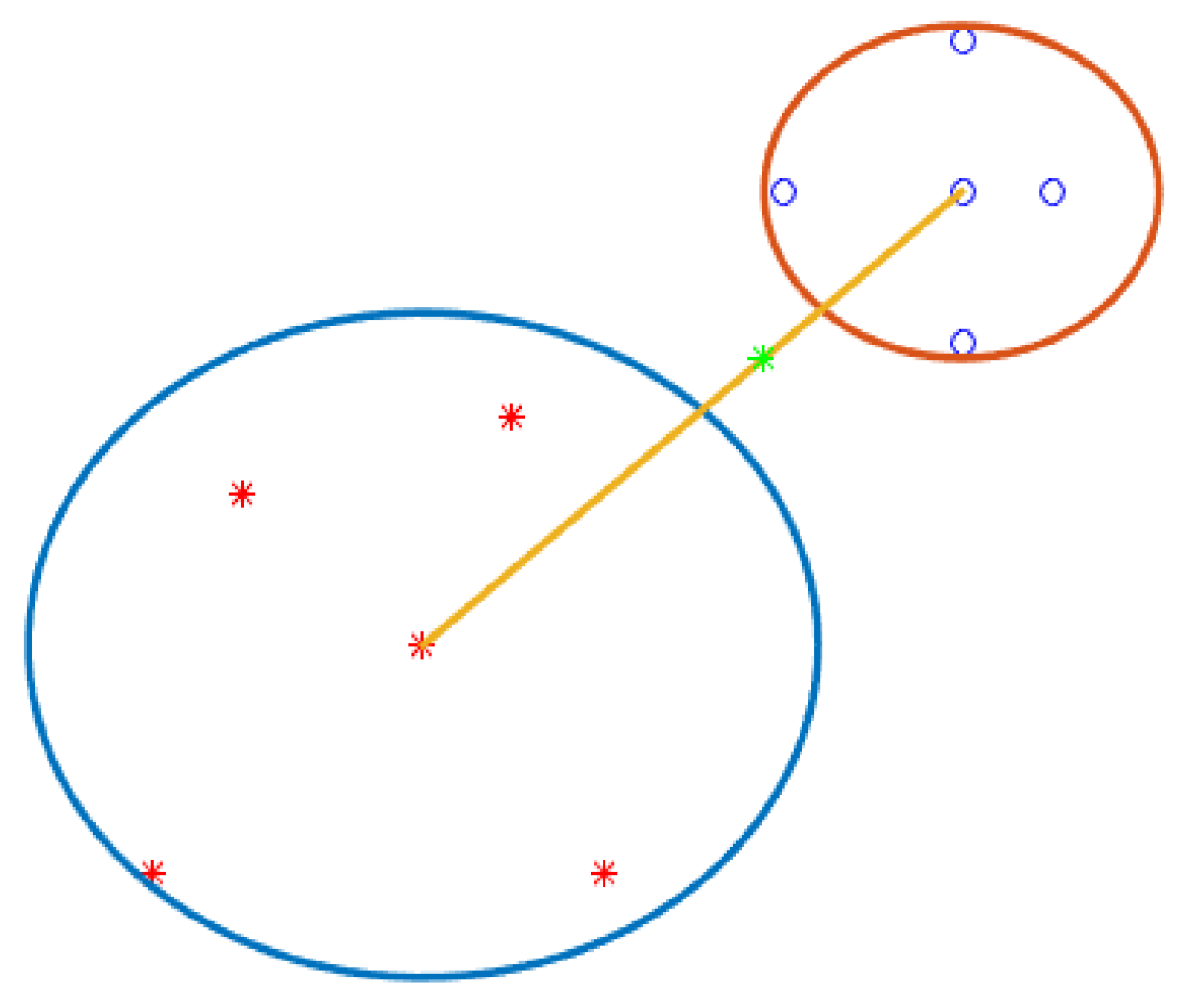
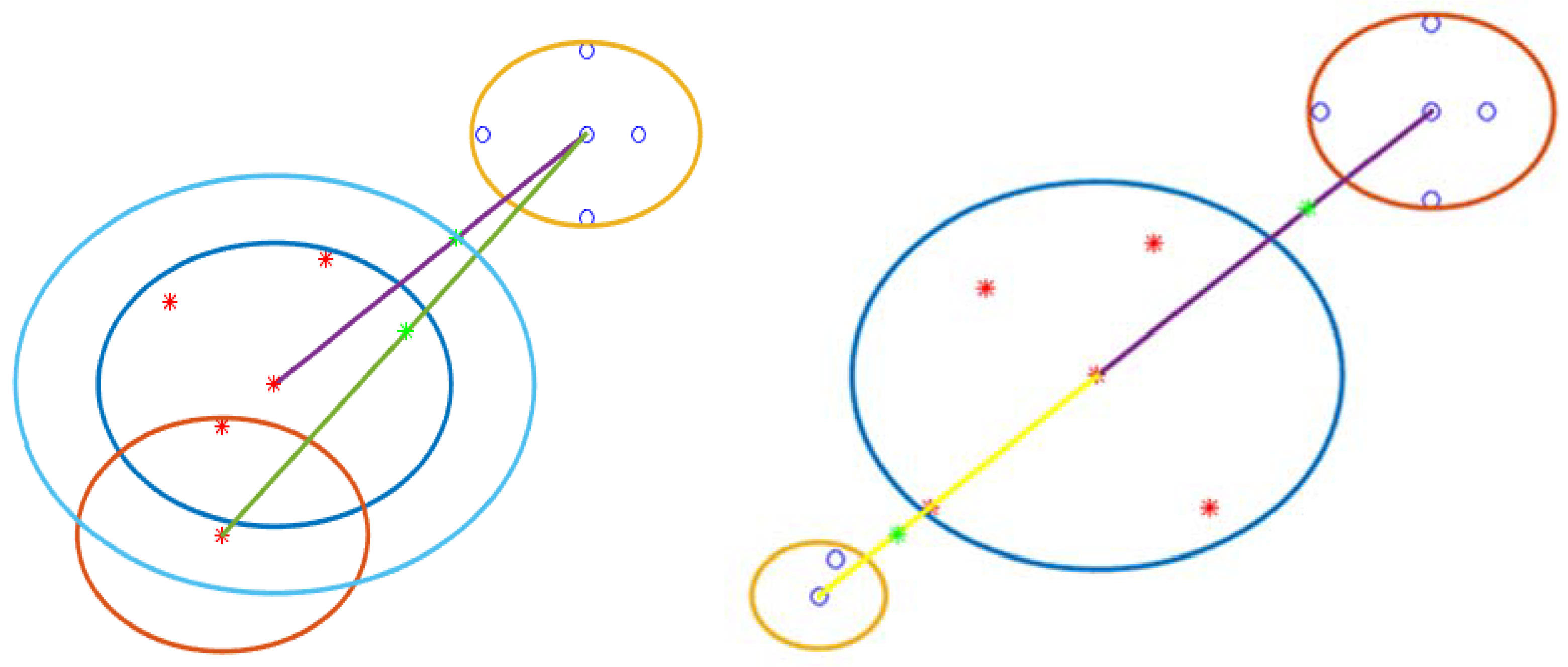
All head nodes of different classes have arches to participate. The distribution of samples in the n-dimension creates the longest different arcs and various centers for arcs. Our model has three modes for detecting a boundary point. 1) Near the center can detect the border point. 2) The local center can detect the boundary point. 3) Near the node center, can recognizes the border point. In one case, it can find the boundary point for arches when the arc does not intersect. The distance between two different central classes calculates. It does not have an arc distance, in the middle of which the distance between nodes recognizes as a boundary point. Figure 12 can show two different class centers. The blue and red dots respectfully belong to classes one and two. The two centers connect by a yellow line (the yellow line is the distance between the two centers). The red arc of class one and the blue arc of class two do not have a cross, and the border points with the green dot are in the middle of the two arches. Other states of the arc have intersections, in which case the arch must break and turn into small arches because only in the first case can this method detect the boundary point. This situation occurs when the distribution of samples is more at the border. The main question is, which arch needs to break? In Figure 9, there are four modes for this situation. All of them are necessary to break the blue arc into two small arches. (Figure 13).
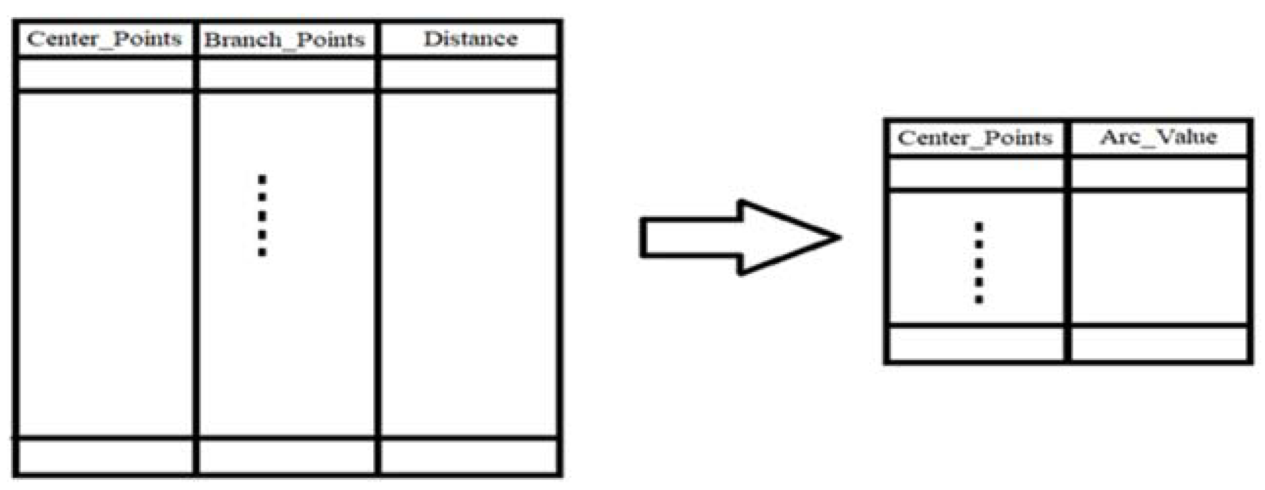
After finding all the border points, some border points are not necessary. Therefore, they need to remove. In Figure 14, two class two arcs and one class arc have two boundary points. One part of the program recognizes that some arches are necessary to stay, and another must delete because one boundary point also supports another boundary point. One green border point on the blue arc is light, and the other is the arc. It means that when two boundary points are in one direction, the other supports the other. In Figure 8, two different directional boundaries and locations do not remove another boundary point. You might think that if another green dot in the blue-green dot arc was bright, another green dot should remove. It is essential for boundaries to remove some boundary points where only a Class I arc has some boundary points with some different Class II arcs. Class two is the same as class one. Our model stores tree data like a matrix to find the longest arc. Then create another table for it. Since arches and centers work together to find the boundary when it is about to break, You must return the first table to create two other (Figure 15).
Then it finds the center of the hypothesis. First, the mean of two or more sample classes finds separately. Second, our model finds the distance between the central and the assumed points. It can see that 50 local concentrated locations are near the center of the hypothesis. Then it computes another hypothetical center based on these local focal points (the sample distribution is closer to the center. But it cannot find it exactly. Because it also has noisy samples. It is impossible not to have noisy features for EEG signals. Our model has a central assumption, then it adds the boundary points (around) of this center, and the other local center has noise, which means that the local and general nodes are noise because the node headbands support sub-nodes. Calculate the distance between the hypothetical axial and noisy axial points and calculate the existing noisy calculation.
In the following, our model has fully explained this classification.
Firstly, it explains the peso code of this model.
In the second step, the flow diagram clearly shows the details of this model.
1) Data collection: Collection of data from each field (collection of signal data from different areas and EEG signals (brain signals)).
2) Input data model (function): Two models intended for sending classification. 1) Raw data sends a classifier directly for classification (raw image data). 2) Processing data as filtering raw data sends the classifier for classification (filter signals). 2) Extract new features of raw data (raw image data and filter signals).
3) Select a data model for classification (function): This supports all models. In test marks, there are two models. 1) Data includes train and test data. 2) K-Fold model in which data divides into K parts. They consider one part of the test and the other part for training. All parts one time considered for testing. It executes K time.
4) Separate class data and random selection vectors (function): Two multi-class models can choose. 1) A class is first class, and other classes are a second class. It runs all these classes one by one. 2) A class is first class, and other classes are a second class. Once executed, that class deleted, and other classes used as public classes. Again, one class is considered a first-class general class and the other a second-class class. Our model runs until all classes are considered first class (First class). It executes these classes one by one.
5) Find the minimum routing for each class (function) separately: All vectors of each class passes to function of the Prim algorithm (it is possible to implement a new algorithm for this idea. But in the first our model uses the Prim algorithm for our purpose.) Each vector is considered a node that has all information of the vectors. The output of a connection matrix is the nodes have the least routing, the first column is the number of nodes, and the second column is the number of neighbors, which includes the least routing. There is no number of leaves in the first column. They exist only in the second column. The original algorithm uses the Euclidean distance to calculate. This table arranged for further processing.
6) Create Arc (Function): Based on the last step matrix, this function creates an arc based on two models. 1) A arc of each node is created from the first column with the maximum distance of children. The high distance between children plus the amount of epsilon considered the size of the Arc to create in all dimensions. 2) A arc is created only in the first column with the maximum distance of children, and they only support leaf nodes. In this type, like the first model, the high distance of children plus the amount of epsilon is also considered the size of the arch to create in all dimensions.
7) Find centers and calculate boundary points (function): This function starts to find boundary points using centers and arcs of two classes. Finding boundary points involves three possible modes, which briefly describe in this section. These modes are in order:
7.1) this means that the boundary point is in the middle of the distance between the two arcs. The Euclidean distance between two equal:
Euclidean Distance = the size of the center arc (Class 1) + the size of the second center arc (Class 2) + the outer distance between the two arches
These expression nodes in the two arches are completing noiseless.
7.2) If two arcs of two different classes are in contact and cover equal or less than a quarter of the other arc (area under the supporting arches) (this means that the Euclidean distance between the two centers is less than The first arc is plus, the center (the size of the second center arc). This mode is divided into two different models, respectively.
7.2.1) this model occurs when two centers do not locate in other arcs. In this case, the nodes belong to each center and its arches and do not place another. These nodes remove two. Other nodes consider finding boundary points. Ineffective nodes remove. They also do not have noisy knots. Noisy nodes are for border-to-border separation. Nodes and Central Nodes Special nodes with epsilon arcs of each class start finding boundary points (all nodes are central nodes with epsilon arcs).
This paragraph of our idea wants to prove the minimum and maximum nodes that can supports by the central nodes.
If the Euclidean distances a and b are equal to the Euclidean ab. Two modes occur. Mode 1: If node 3 is in zone 1, the central node cannot support node 3 (meaning that Node 3 does not have the minimum path to the central node). Mode 2: If Node 3 is in zone 2, Node 3 can support by the central node (this means that Node 3 has the least routing to the central node). But Node 2 can be supported by the central node. Node 2 connects node 3 (has minimal routing). If this path continues to all the space, the central node can support more nodes.
It does by examining the nodes with far and near distances. Each node can support angles between 60 and 120 degrees. If it considers the average of 90 degrees indicates that the number of nodes can be increased or decreased. But the number of nodes cannot increase the constant value, and if the minimum degree (60 degrees) or maximum degree considers for the nodes. The number of nodes is six nodes and three nodes, respectively.
7.2.2) When this model occurs, two arcs are touched. The big arc cannot fully support others (the small into the big). Under these conditions, all nodes are considered central. Then all the nodes go to the first mode and find the boundary points. These knots are a bit noisy. It exists right on the border. They may go to another class a little.
7.3) In this case, the center of the first class with its arc is placed in the center of another center class (meaning that the large fully supports the small. The Euclidean distance is also less than the arc scale. The Euclidean distance equals the absolute value of the size of one central arc (Class 1) minus the size of another center arc (Class 2). Use only the central node to find the boundary points. But another center breaks, and all nodes and centers become center nodes with epsilon values for their arcs. To the nodes, These nodes go to mode 1 to find the boundary points. Based on the Mathematica formula described above. The nodes locate away from the support of the other arc zone. These nodes remove before sending mode 1.
8) Effective and inefficient central boundary detection (function): This function supports two modes. 1) Boundary center detection for classification: All centers identify in the first case. But they are not exactly in the border area. They are not used to find border points. They removed. All centers in modes 2 and 3 are designed to find border points. 2) Identify the public center of each class: For all centers in the first case and all centers in the border support area to find the border, they are removed based on the deletion method. Based on the ranking of the total centers, the calculation leads to our center can find, which is close to the public center (it may have a central center. And then divide the sum of all ranking values). Find the general center assumption for calculating the noise intended for each node and will apply it to future work.
Figure 10 shows the flow diagram for the classification and noise detection of the two classes. This model becomes a multi-model by repeating this flow chart for more classes. For example, there are three classes. In Stage 1, the first class is Class 1, and the second and third classes are Class 2. In stage 2, the second class is class one, and the first and third classes call class two. In Stage 3, the third class is Class 1, and the first and second classes call Class 2. In this flowchart, our classifier uses the prim algorithm to find the least spanning tree. Anyone can use any algorithm that has a small chronological order. The best effect of this idea is that our model can use it as a steep descent to expand backward. For example, writing this idea and choosing a feature can be a great feature. And the sample noise is correct if more than 60 creatures do not have noise. The performance of this classification is more than 70% which is very well accuracy, and less than 50 is the worst. This classification is not very suitable for noise detection.

2.4. Deep Formula Detection With Extracting Formula Classifiers

2.4.1. Classification of deep formula coefficients by extracting formula coefficients in different layers along with prevalent classifiers

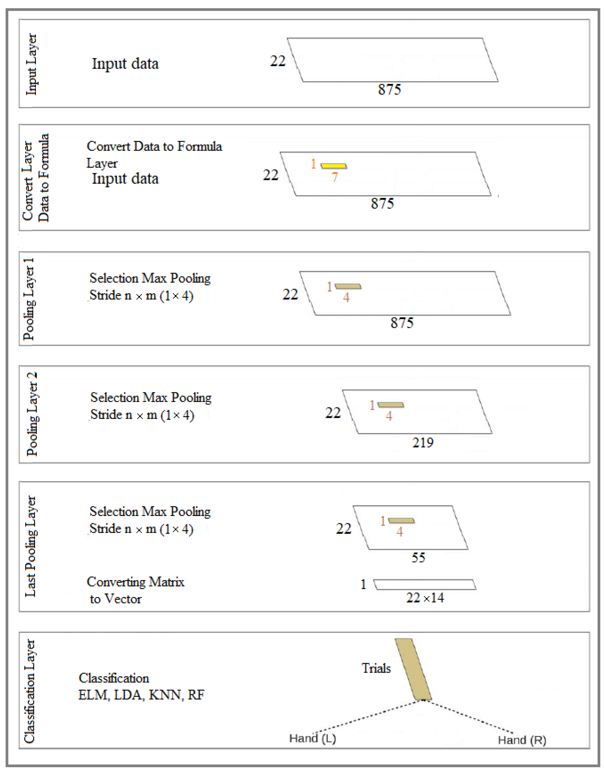
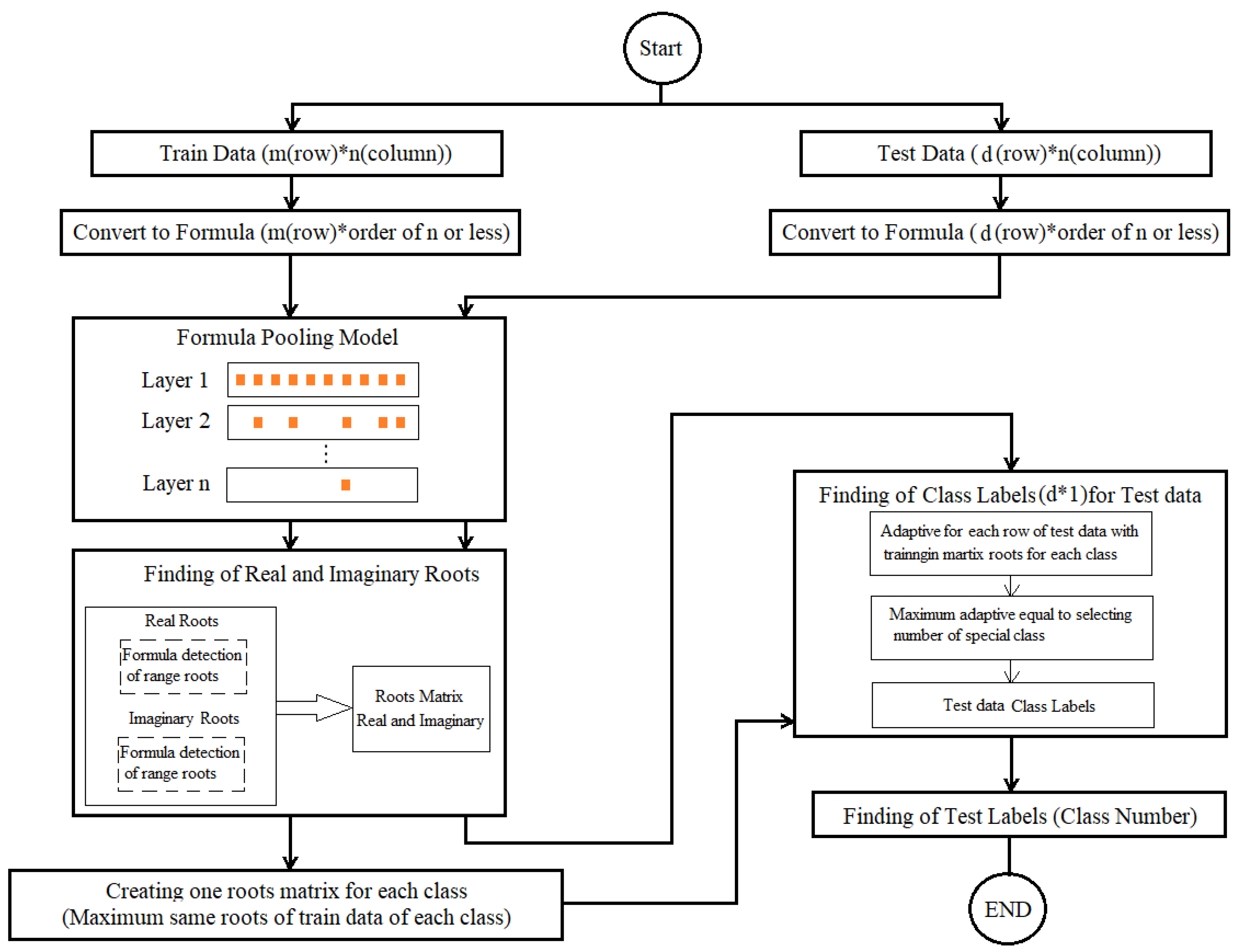
This section introduced a new model which converts the data into a formula in the first layer, and then the coefficients are extracted and selected in the other layers. After the last layer, the selected coefficients are sent as coefficients from the main formula to various classifiers. It is possible to apply classification to them. This model includes the following steps for definition, which are: (Figure 6):
1) Data-to-formula conversion layer: The input layer is the input data-to-formula conversion layer. At first, windows with specific sizes define to convert data into formulas, and then the conversion is done. In other words, the data converts into a polynomial equation using Lagrange’s formula based on the defined window size (filter in deep learning). The jump also uses in such a way that they do not overlap. In this layer, the entire matrix or vectors convert into formulas.
2) Formula coefficients selection layers: These layers are defined similarly to convolution neural network layers to remove noise from coefficients. But in this implementation, only the sampling part is used for layers (sampling without noise removal using convolution neural networks). When the sampling function (without noise removal) uses in each layer. The only method of separating specific parts of polynomial formulas based on specific criteria is applied. In other words, the coefficients of formulas decreased. We have implemented this model as a prototype for our research.
3) Common and common classifiers for data: In this part, several common and common classifiers RF, KNN, SVM, and LDA used.

2.4.2. Detecting the range of deep formula roots by extracting coefficients of formulas in different layers along with the extraction of the roots ranges together with the classifiers of event formula roots

This section presents a new model which the data converts into a formula in the first layer, and then the coefficients are extracted and selected in the other layers. After the last layer, the coefficients are selected as coefficients from the original formula to the new interval extraction model. Test formulas sent to have classification applied to them for the same root interval basis. This model includes the following steps for definition, which are: (Figure 16):
1) This layer is the same as the items defined in the first part of the section 2.2, which uses in the same way for the two specified items. The only difference can be the various selection of the coefficient selection function in different layers.
2) These layers are the same as those defined in the first part of the section 2.2, which uses in the same way for the two specified cases. The only difference can be the various selection of the coefficient selection function in different layers.
3) New classifier based on the rooting interval of formulas for classes: a new classifier introduced to extract and identify the roots of group members as a class based on the formula roots of the majority of members. In this way, the range of majority formula roots of members of each class is identified and recognized during learning. Based on the high similarity between the formula roots intervals of the experimental members using the root interval of the group members (classes), it is possible to identify and determine which belong to group members a class. Our experiment runs on the members of two classes.
Because it takes a lot of time to find the exact place of roots, for this reason, we have chosen the method of finding the roots of equations or polynomials at specific intervals, which requires less time. It does not need to find the exact positions. But we can discover roots at certain fixed and limited intervals where there is a root in this interval. Our classifier uses certain fixed bounded intervals of formula Roots instead of the exact place of formula roots for classification. Formula Roots are in certain fixed bounded intervals.
In the following, it is described new roots extraction and detection classifiers for more details.
Suppose the function f is given by the table in the figure below so that we have for i j : x i x j In this method, we assume that L 0 ( x ) , L 1 ( x ) , , L n ( x ) each is a polynomial of degree n.
P ( x ) = L 0 ( x ) f 0 + L 1 ( x ) f 1 + + L n ( x ) f n
Where we have n for j = 0 , 1 , , n .
L j ( x ) = ( ( x x 0 ) ( x x 1 ) ( x x j 1 ) ( x x j + 1 ) ) ( x x n ) ) ( ( x j x 0 ) ( x j x 1 ) ( x j x j 1 ) ( x j x j + 1 ) ) ( x j x n ) )
We have.
L i ( x i ) = { 0 ,   i = j 1 , i < > j L i ( x i ) = { 0 ,   i = j 1 , i < > j
So we will have.
P ( x i ) = f i ,   i , 0 , 1 , , n .
That is, the polynomial (x) P defined by (1) holds in the condition P ( x i ) = f i .
The model for finding roots in a range is that the equation is divided into certain intervals. The range that has the condition of having a root is known as the root range, which must have the following conditions.
The following equation is used for real roots.
O 1.. m = ( a n x n + a n 1 x n 1 + + a 1 x 1 + a 0 ) ( x + b 1.. m )   .   i , j , n = 1 m .  
The following equation is used for imaginary roots.
O 1.. m = ( a n x n + a n 1 x n 1 + + a 1 x 1 + a 0 ) ( xf + b 1.. m )   .   i , j , n = 1 m , f = 2 , 4 , , d
We use the following method to establish the condition of the existence of the root in the specified interval.
If | O i | = | O n | and | O n | = | O j | , and ( O i is positive and O j is negative) or ( O i is negative and O j is positive), i < n < j Lead to one root is n value range.

2.4.3. Dataset and Experiments

Dataset IIa [101], from BCI competition IV: It is included EEG signals from 9 subjects, and they performed four class imagery such as left hand, right hand, foot, and tongue motor imagery (MI). 22 electrodes for the recording of EEG signals on the scalp have been used. For our research, EEG signals of left and right-hands MI are considered. All training (72 trials) and testing (72 trials) sets are available for each subject. Our experiment used 280 trails. For our research, it is considered 10-10fold for experiments. This dataset is used for all four ideas.
The structure is easier to find the roots of the equation or polynomial in specific intervals. It means that it does not find the exact position of roots, it finds roots in fixed limited specific intervals and the current commonly used classifiers use different formulas to differentiate the extracted class property.
When entering the coefficients of the formulas into the classifier, the coefficients of the training and test formulas are separated with a specified function. This method is also executed with the Kfold10-10 method.
The root classifier detection section (test function) identifies the roots of the classes based on the most similar formula roots between the members of the same class, so the formula roots of each class are identified and recognized. Each test member belongs to a class that has a high similarity between the formula roots of that member and the roots of one of the classes.
This section describes the values assigned to variables and structures for practical implementation. This includes:
1) All filter banks (1 to 9) with three selected channels (8, 10, and 12) are used to run the models.
2) Two fixed window sizes (7 and 14) are used, which convert data into formulas in the first layer.
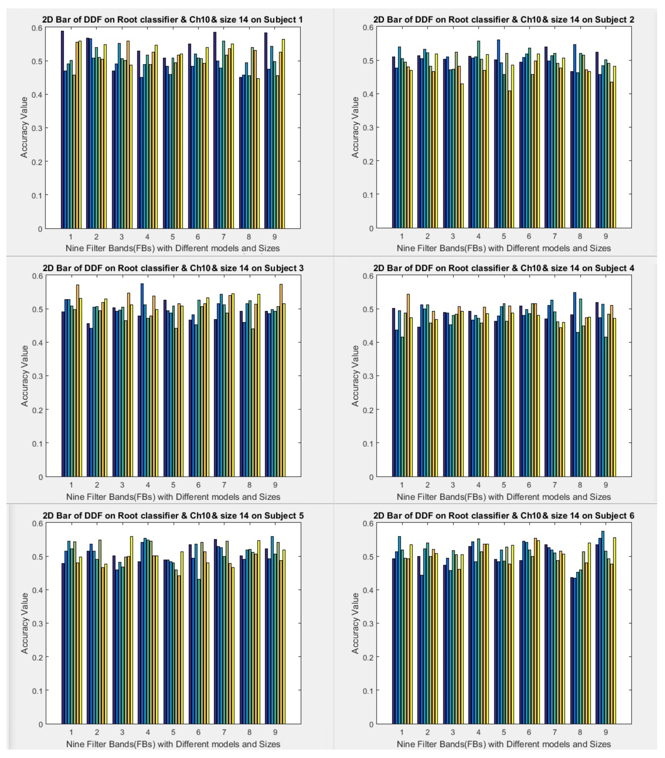
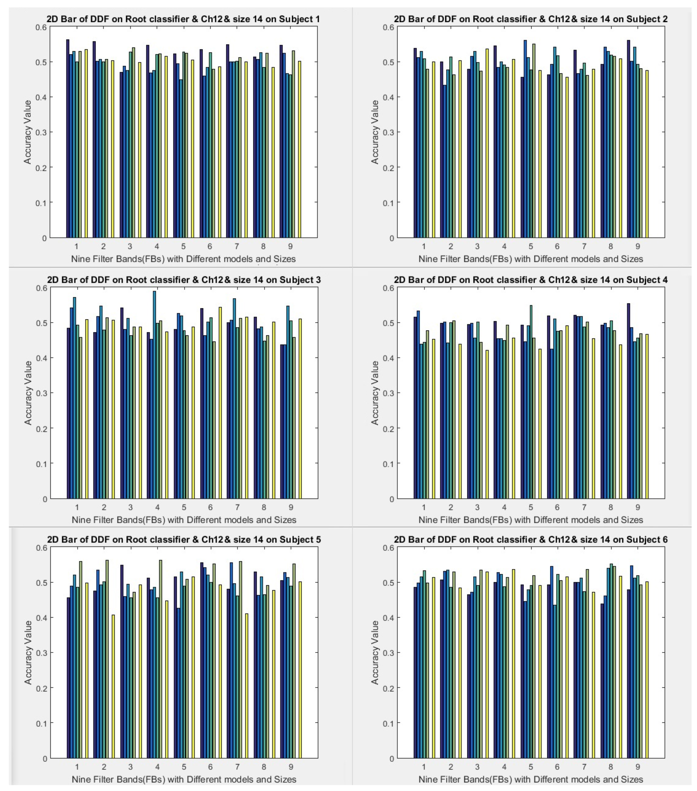
3) Window sampling size is used for the second and subsequent layers, respectively 3, 5, 7, 10, and 15 for size 7 (data to formula conversion). The window sampling size for the second layer and subsequent layers are 5, 10, and 14 the size of 14 (data to formula conversion), and various variables use for investigation. The results of the two cases mentioned above obtain. But this article shows the formula with a window size of 14.
4) The root folder has ten folders and ten executions. On average, all the results of 10 folders after execution are considered the final result. Therefore, it executes ten times, and the average of ten times is considered the final result. For the classifier, we set the root range (spin range) to 0.5 and can set it between 0.001 to 1. But the smaller the interval of these roots, the more time it will take to find the formula roots (our model considers only one mode).
Next, you can see an overview of the proposed new model with prevalent classifiers in Figure 17.
The size of the output layers and the filters used in four ways:
1) In all models, the input layer includes 288 mental images, nine filter banks, 22 channels, and 875 features for each channel during a mental imagination for each brain activity as left or right-hand. In other words, the total input data is 875x22x888x9x288 for a specific image such as the left or right hand. Therefore, the features are extracted from the original signal for each filter bank separately. In other words, the primary data stored by the electrodes for the EEG signal for each specific mental imagination (left or right hand) is equal to 875x22x288.
2) The second layer uses to extract spatial features. This way, a 22 x 1 filter applies to the channels, the output of which is 288 x 875. For all nine bank filters, feature extraction does separate. The second layer output for all models is 288x9x1x875.
3) The third layer removes in one of the models. So the third layer implements in two models. The third layer acts as an RNN layer. The jump operation is the same as the window size (filter size). The output of all models is 175x1, which includes two matrices in the form of a screen and nine bank filters, and the total network output results are 285x9x1x175.
4) The third layer uses only one model (the first model). The third layer input (the output of the second layer) directs to a fully connected neural network (MLP). The size for MLP is a 5x5 matrix. The last layer output is equal to the input to the neural network.
5) The data output of the last layer is collected for classification, and if it is in the form of a matrix, it converts into a one-dimensional vector. The number of features is equal to m, and the number of repetitions of brain activity is equal to 288. In other words, 288 × M, where m represents m = 175 × 2 × 9. Finally, a two-dimensional matrix sends to the classifier.
6) In the model where the third layer is disabled. The output of the second layer is sent directly to the ELM classifier for classification. The input data randomly divide into 50% and 50% training and testing parts. 20 neurons use for the ELM classifier.
3. Experiments and Results

In this section, we present the experimental results and analysis for our proposed models. Based on the experiments, these models can improve accuracy and kappa, and decrease the noise for extracting good patterns in large-scale frequency bands (4-40Hz). They also contribute to increasing the distinctive patterns between two activities by increasing the scale of filter banks. All models are implemented for left and right hands data, and the first model is implemented for both hand and foot data. The results are described in the following sub-sections.

3.1. Datasets and Experiments

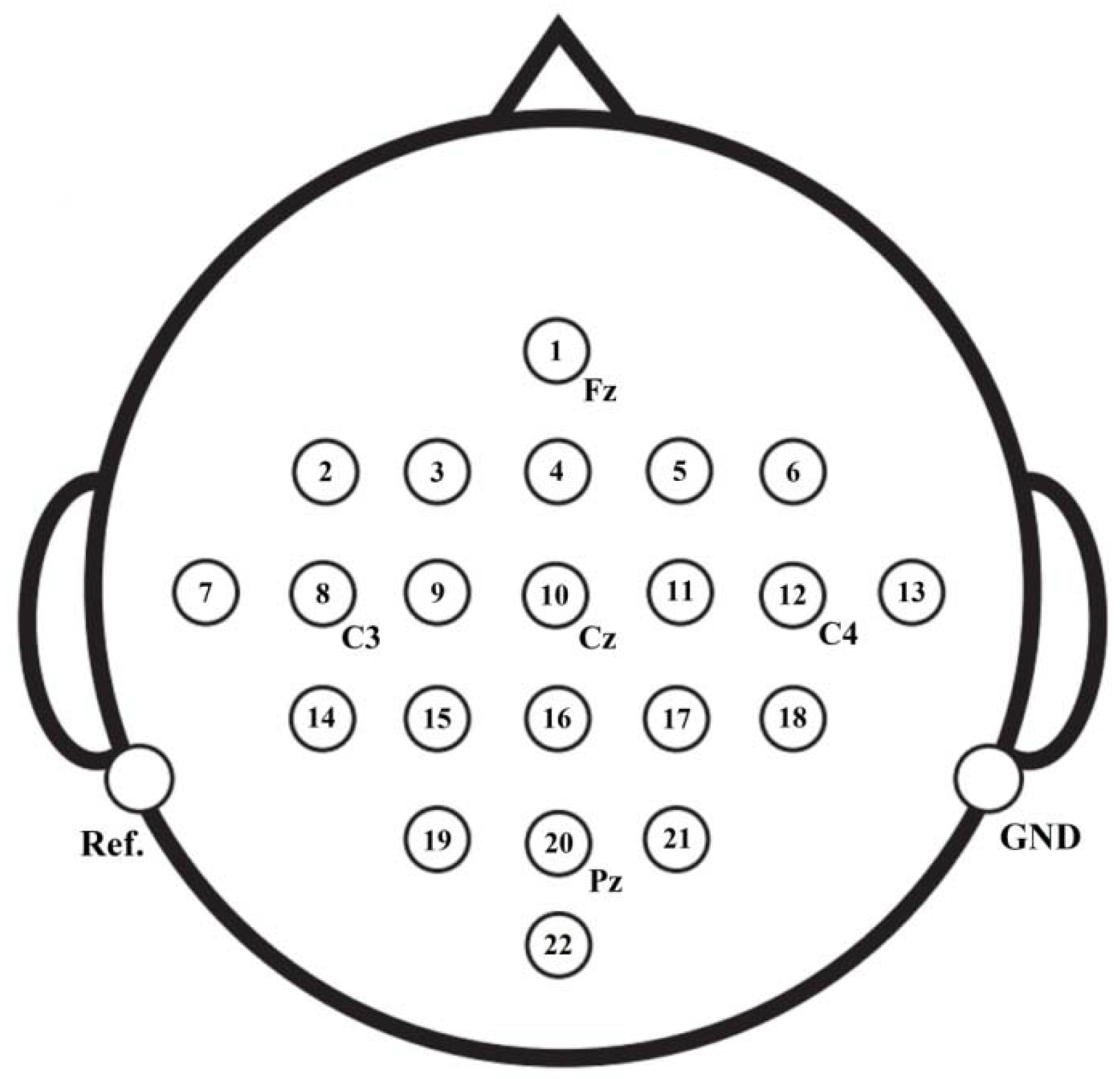
1) Dataset IIa [97], from BCI competition IV that includes EEG signals from 9 subjects, and that are performed four classes of imagery such as left hand, right hand, foot, and tongue motor imagery (MI). Twenty-two electrodes for the recording of EEG signals on the scalp from this dataset have been used. For our experiments, EEG signals of left and right hands MI are considered. All training (72 trials) and testing (72 trials) sets are available for each subject. Our experiment used 280 trails. We evaluated 10-10 fold (cross-validation) in the experiments. This dataset is used for all four proposed models. Figure 18 shows the location of selection electrodes on the scalp of the brain in IIa of BCI competition IV.
2) Dataset IVa [98], from BCI competition III [99] that includes EEG signals from 5 subjects, including right hand and foot motor imagery (MI). One hundred eighteen electrodes for recording are used. All training (140 trials) and testing (140 trials) sets are available for each subject.
We applied 10-10 fold cross-validation for training. The integrated training and validation data is considered for or training and test. The whole integrated data is divided into ten folds randomly. Each fold is applied as test data once, and the rest are considered train data. The procedure is repeated ten times, and averages of results are considered as final results. We use Butterworth filter with 100th order for filtering. We restricted our experiments to the data between 0.5 seconds before the visual cue to 3.0 seconds after the visual cue. So, we used 3.5 seconds, and each second includes 250 features (points). In total, all of the input features of each trial for one electrode are 875 features.

3.2. CSP Using New Combination Signal

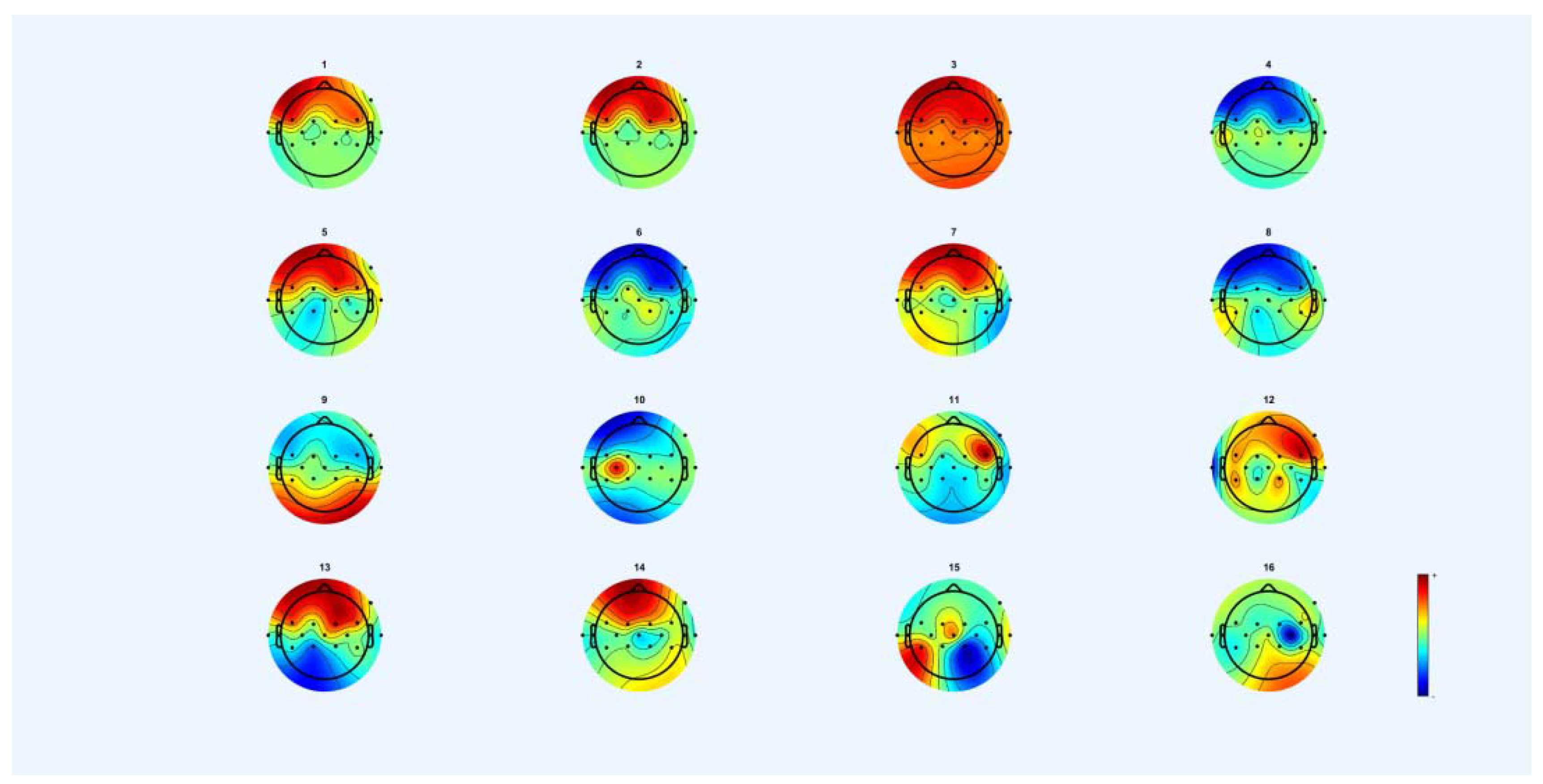
During the test period is 9 seconds, the signals of the image period contain only good information. Our paper shows the time-frequency analysis of EEG signals of the image period, which show the outstanding performance of the image period with the time window on the running image scale. ICA breaks down the channel data into interdependent components based on the training data. The number of ICA components is automatically selected based on the classification function in the training method (measured with mutual accuracy), which is physiologically appropriate because the neural sources of the ICA components are likely to be mutually independent and independent of ambient noise. Thus, significant neural components associated with movement/imaging are relatively amplified compared to unrelated neural components and noise (Bai et al., 2007).
To demonstrate ICA-amplified neural signals, it created four samples of ICA topography. Many aids identified from the sensory areas and formed in a circular shape which reflect our system’s emphasis on motor signals.
The ICA spatial filter attenuates the EEG signal in some parts of the scalp and amplifies the EEG signal in other parts of the scalp. To visualize typical signals amplified by the ICA space filter, is created ICA topographic diagrams for one person (person number one) and two mental images created as graphs. For classifying the two images, diagrams show which areas of the scalp have been weakened and which have been strengthened. A classification is made up of each chart because the weight and number of components of ICA components differ between classifications due to different training data (Figure 19).
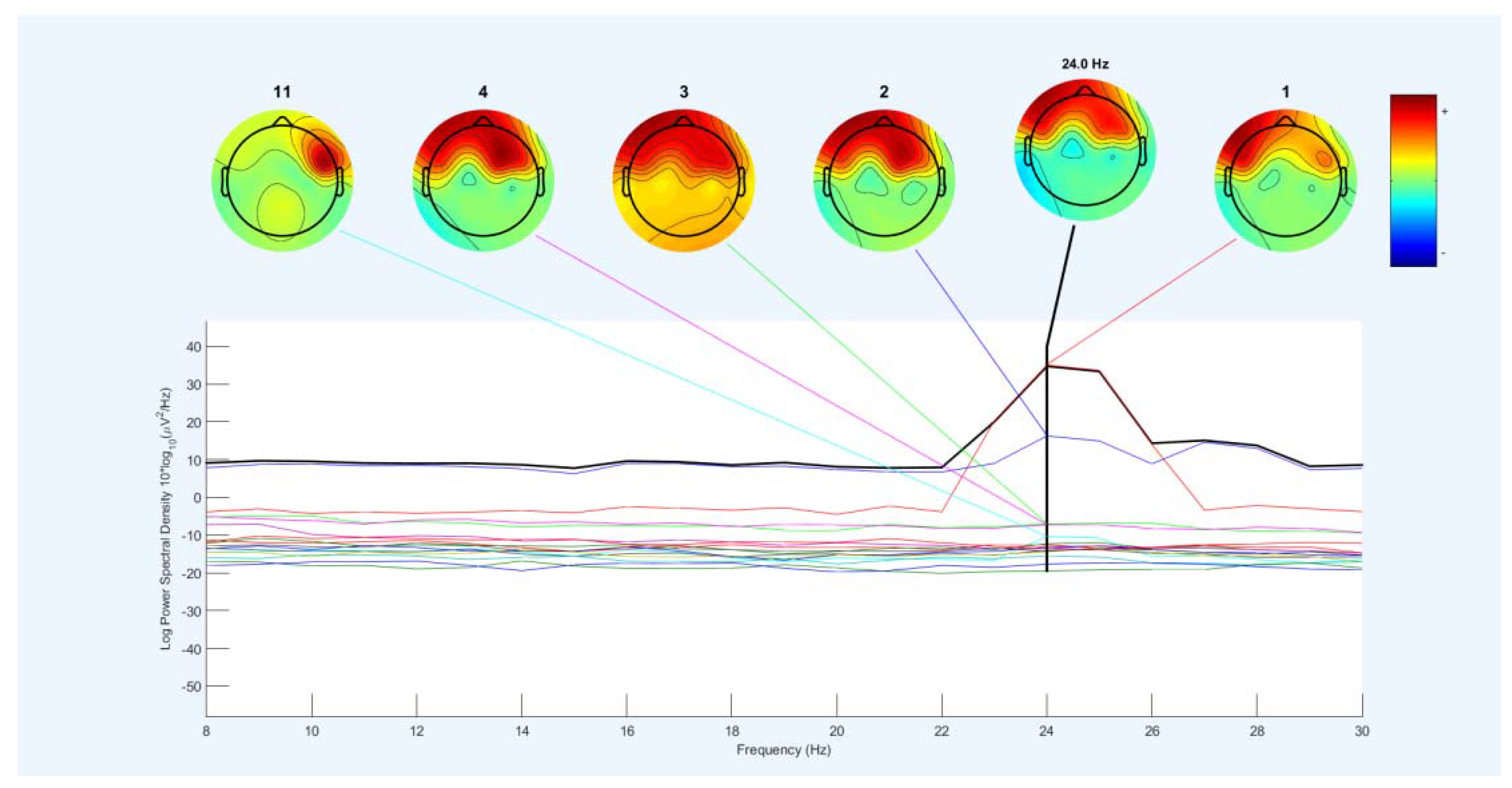
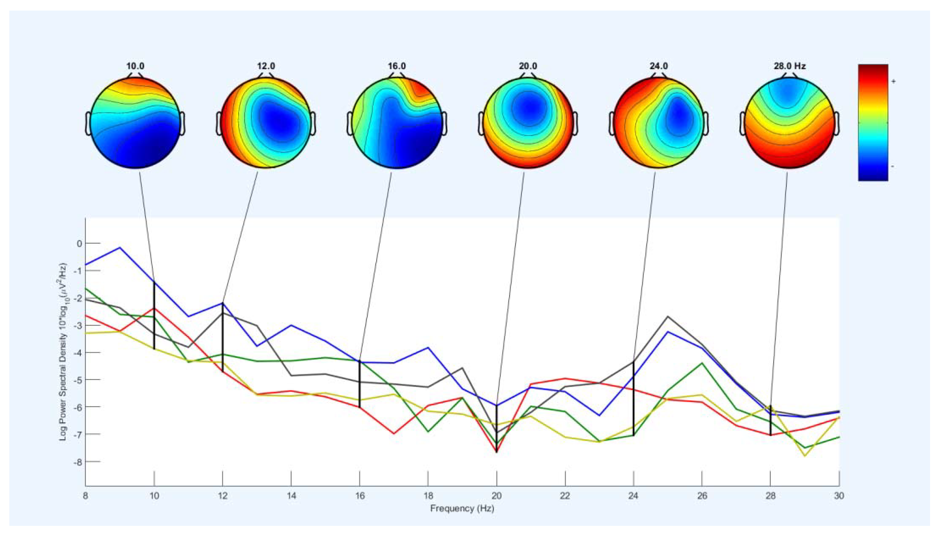
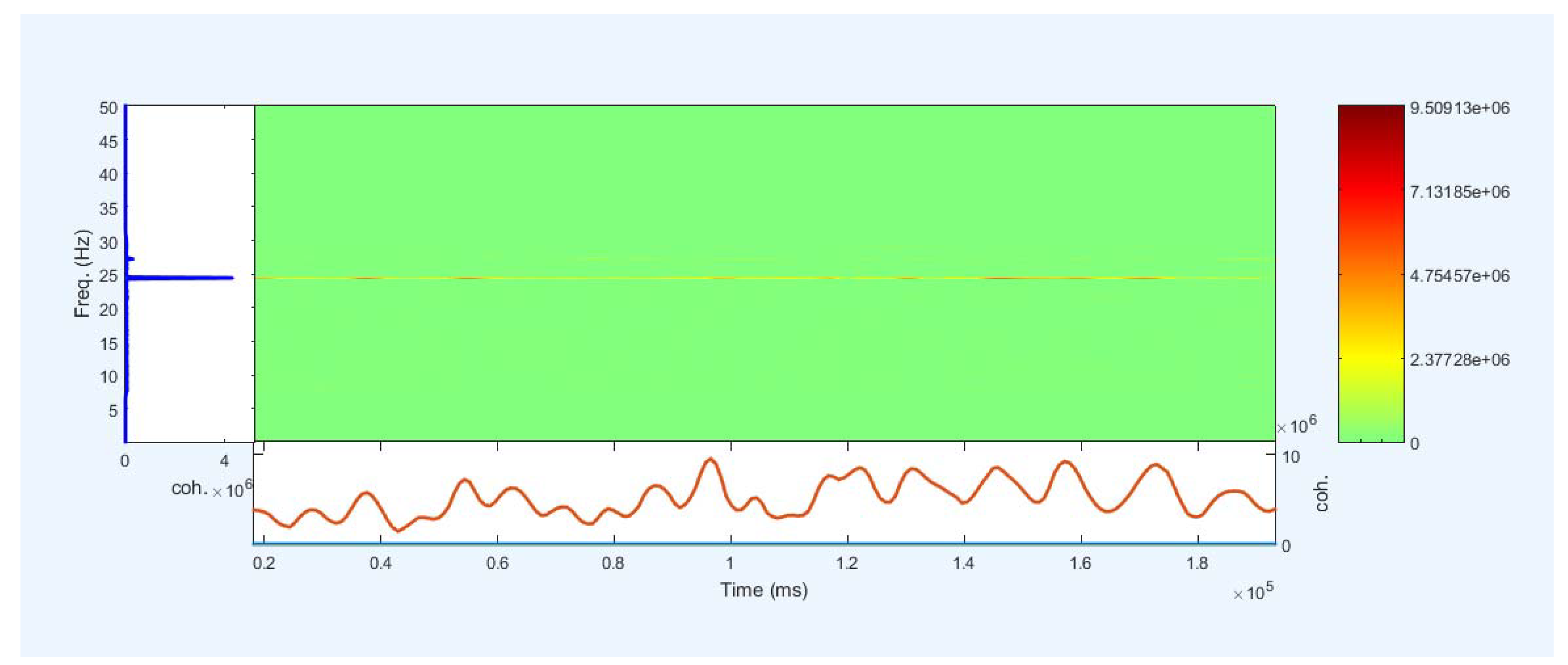
Figure 20 shows a frequency diagram with the power of the spectrum in the frequency range of 8 to 30 Hz. It examines 16 channels for the two lip-reading concepts "A" and "M" in EEGLAB. The power spectrum obtained between 10 to 20 in the frequency range 8 to 22Hz. Between two intervals is a little less and returned to the original state. These intervals are between 14-14 Hz and 22-20 Hz. Then, between 24-22Hz, the power of the spectrum increases to 40 Hz. First, between 25 to 24 Hz with a slow slope decreases slightly. And at about 25Hz, it goes down with a steep slope and reaches 20. And between the range of 28-26, it goes up and down a little, and then the frequency comes back the power of the previous intervals, which indicates the power of the spectrum in this range, which increases during imaging.
Figure 20 shows a frequency diagram with the power of the spectrum in the frequency range of 16 to 36 Hz. It examined 16 channels for the two lip-reading notions of A and M in EEGLAB. The power of the frequency spectrum increases and decreases between the frequency range of 22-25, which increase up to 40Hz, and after the frequency range of 33 Hz, they return to the lowest negative. Between 16 to 30Hz, the power of the spectrum increases. This interval corresponds to the mental imagery interval. Different channels show the energy at 25 Hz on the head. Therefore, this indicates that the power and energy of the brain parts are distinct when mentally imagining at a frequency of 25 Hz. Figure 21 shows the power output as Figure 21. But it is between 8 to 16Hz.
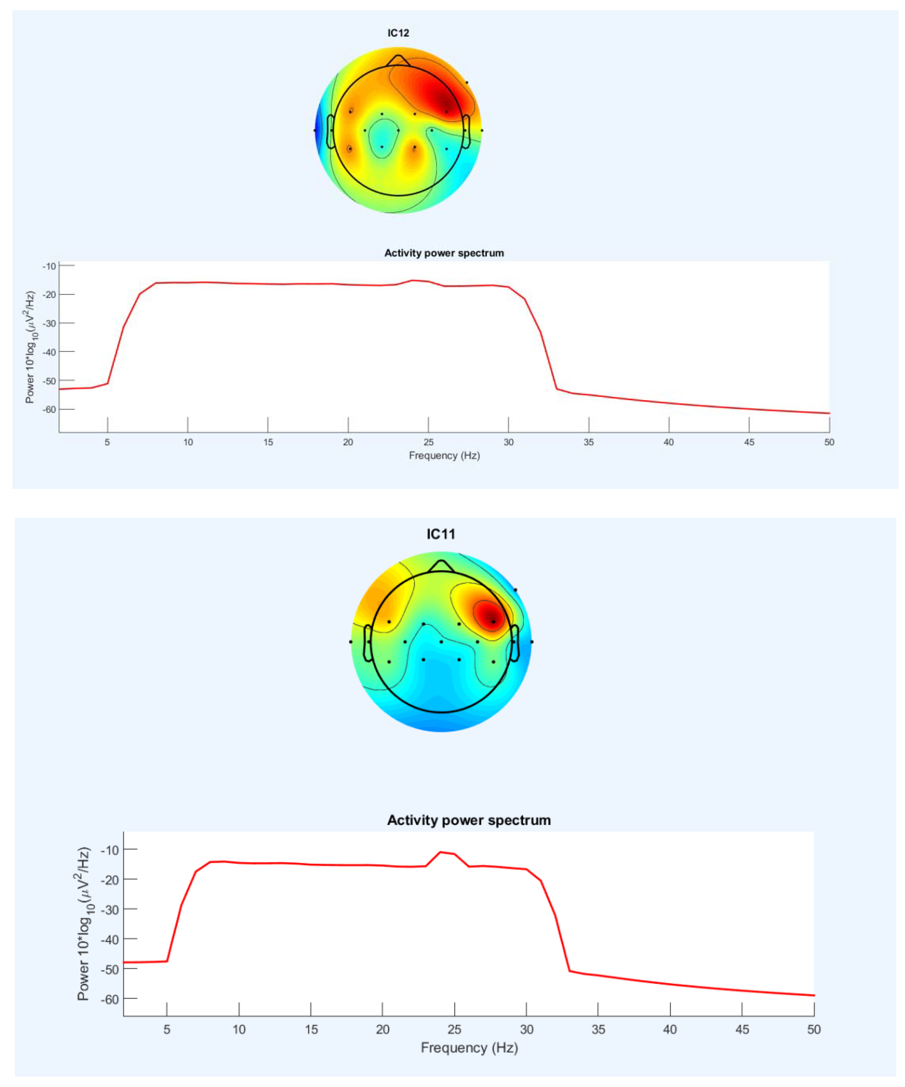
As shown in Figure 20 and Figure 23, Figure 24 examines the frequency power diagram in the 0 to 50 Hz frequency range. Frequency power varies in the frequency range of 4 to 34 Hz. Frequency power increases between 4 and 8, and frequency power decrease between 31 and 34 Hz. The frequency power is almost the same between 8 and 30 but in the range of 23 to 26. There is a slight increase and decrease in frequency. The amount of energy also shows in different parts of the joint. Only one channel for the power of the spectrum is shown.
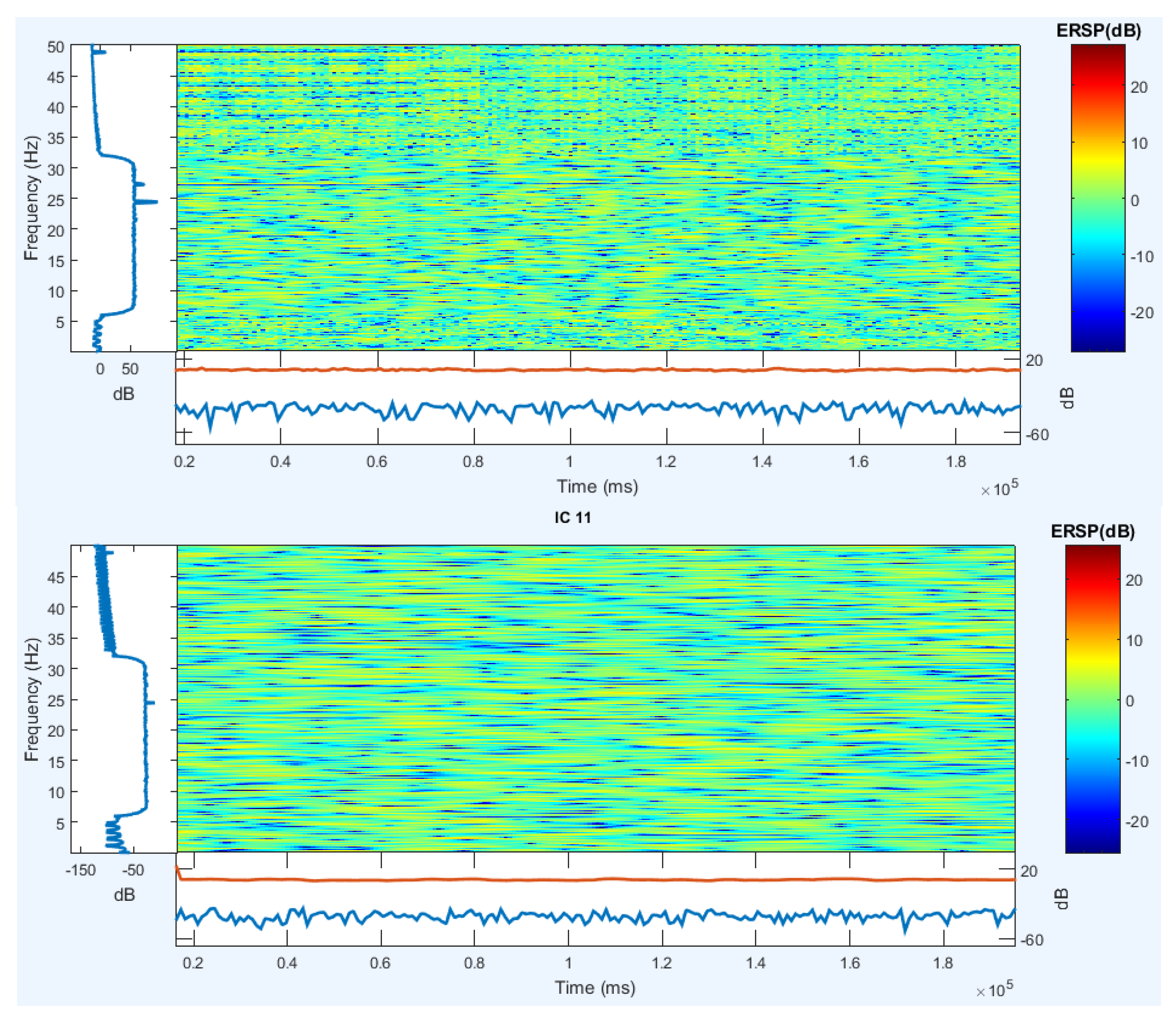
To compare with the previous work (speech imagery and mental task) [100], channels C3 and C4 near Broca’s area and Wernicke’s area are selected to analyze event-related spectral perturbation (ERSP). Using complex Morlet’s wavelets, single-trial had to superimpose energy spectrum by ERSP. EEGLAB was used for plotting ERSP in this dissertation [100]. The ERSPs related to the two channels are respectively presented from subject 1 in the second and third steps in Figure 25.
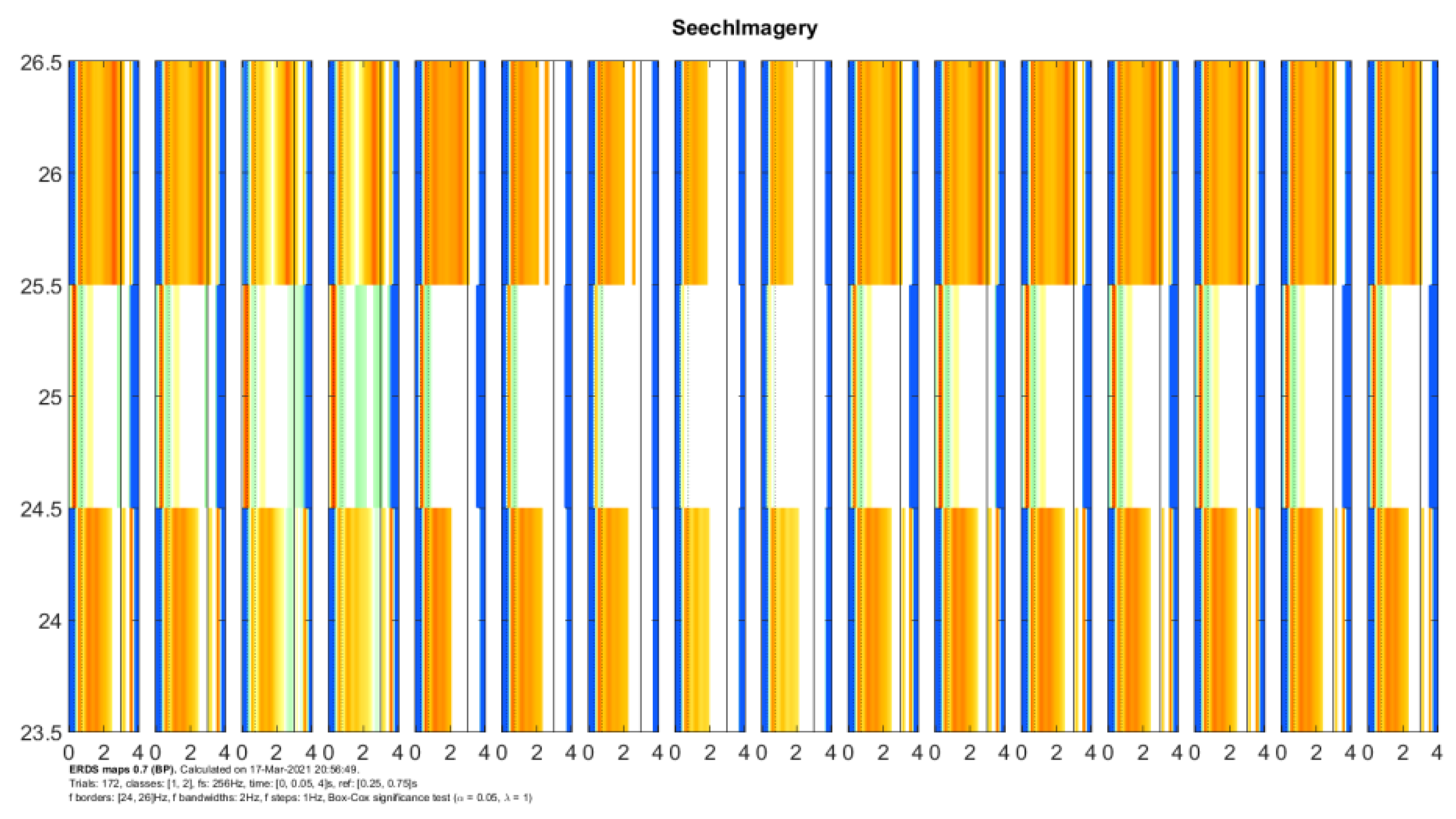
For comparison with previous work (speech image and mental task) [100], like another article in the field of imagination, channel signals were referenced, and all sixteen channels were selected for all areas of the brain, especially the Broca and Wernicke regions. Using the complex Morlet’s wavelet, the experimental experiment has an extraordinary energy spectrum by ERDS. CSP is used to draw ERDS in this dissertation. Figure 26 shows ERDS in the frequency range of 23 to 27 Hz between 0 to 4 seconds. The imagination period for each activity examines separately and for two images simultaneously, and different energy strengths observed for all three expressed cases. Completely different frequency power can be seen between the two notions, and various changes observed between the two intervals between the distances of a frequency range. See Figure 26 for more information. Due to the noise of the signals, the rest of the frequency range has omitted.
Cronbach’s alpha coefficient evaluates the temporal stability of ERD/ERS in Figure 27. During the experiment, the coefficients of the three-time intervals were calculated. The coefficients and the specified yields are constant (> 0.7), respectively, Figure 27.
For calculating the classification accuracy, the EEG signals of any subject used in training and testing sets by 5 × 10 fold cross-validation. The dataset was randomly divided into ten equal parts. Test spatial filters and classification apply for each part of testing, and other parts are used to build CSP spatial filters. Then it is extracted the feature values and train the classifier. The average of ten different accuracies calculates overall accuracy. It also uses fivefold cross-validation. This training/testing procedure is repeated ten times with random detachment. The standard deviation calculates for analyzing. It presented the accuracy rates of the two subjects in Table 1.
The best average validation accuracies of 3D Lips between “A” and “M” from three subjects are between 66% and 70% in Table 1. Subject 1 with KNN has an accuracy of about 68.7% in the best state. The result of Subject 1 is about 54% up to 68.7%, and Subject 2 is between 57% up to 64%. Classification with KNN has good accuracy of 62% to 69% related to other classifiers. SVM looks like KNN is 61% to 68%. It has a 1% accuracy less than KNN. Accuracies of classification from Subject 3 are between two subjects. The signals of the three subjects are enough noise. LDA has minimum accuracies for subjects between 54% to 58% which is weaker. Other classifiers acted well or less.

3.3. New Combination Signal using Four Common Methods

3.3.1. CSP Using New Combination Signal

Table 2 shows the results of ten extracted features as five pair-features by CSP. Three classifiers, including LDA, KNN, and ELM are used in our experiments. For evaluation, we calculate the average Kappa of all subjects for left and right hands. Note that the new combination signals are presented as the combination of filter banks with their numbers. For example, a combination of the filter bank, I, and filter bank J, is expressed as “FB I and J”.
Based on Table 2, In the comparison of KNN and ELM, KNN has the lowest kappa. The LDA to ELM and KNN has a slightly better kappa. The highest kappa value is for FB 5 and 6 (68.70%). CSP could remove noise well and extract good suitable features for left and right. LDA and ELM classifiers are successful for detecting suitable different patterns between two classes while the same patterns for two-class can be more.
In general, Table 3 shows the results of five Paris features (ten features) for subjects by CSP that are performed for our experiments by the LDA classifier. The details of subjects are shown for LDA with slightly better accuracy (left and right hands). Exception two subjects the rest have higher kappa (more than 60%), which declares that some subjects achieved the low kappa value and other subjects achieved the high kappa value.
Table 4 shows the details of the average sensitivity of subjects for some of the new combinations signals. It declares that the difference between left and right-hand classes is less than 2 %. And the difference between sensitivity and accuracy is near with a little difference.
Table 5 shows the results of ten extracted features (five Paris features) by CSP and is performed for our experiments by three classifiers such as LDA, KNN, and ELM. For evaluation, it is calculated average Kappa of all subjects for hand and foot.
Based on Table 5, in the comparison of KNN and ELM, ELM has the lowest kappa. The LDA to ELM and KNN has a slightly better kappa. The highest kappa value for FB 3 and 9 (95.90%). CSP could remove noise very well and extract excellent features for hand and foot. LDA and KNN classifiers are successful for detecting the most different patterns between two classes while the different patterns for two-class are very more based on results.
In general, Table 6 shows the results of five Paris features (ten features) for subjects by CSP that are performed for our experiments by the LDA classifier. The details of subjects are shown for LDA with slightly better accuracy (hand and foot). All of the subjects have the highest kappa (more than 90%), which declares subjects achieved the highest kappa value.
Table 7 shows the details of the average sensitivity of subjects for some of the new combinations signals. It declares that the difference between left and right-hand classes is less than 2 %. And the difference between sensitivity and accuracy is near with a little difference.
In Table 3 and Table 6, the results of the p-value for our proposed method (new signals & CSP) with LDA classifier based on CSP (C3, C4, CZ)[101] are calculated for left and right hands, and hand and foot. In Table 2, for FB 5 and 6, is calculated 0.002 less than 0.05 and others p-values (p-values=0.002). In the second level, FB 5 and 9 could have 0.003 (p-value<0.05). In the Table 6, for FB 3 with 9, is calculated 0.0061 less than 0.05 and others p-values (p-values=0.0061). In the second level, FB 4 with 9 could have 0.0058 p-value (p-value = 0.0058). It is shown the newest combination signals are statistically significant for left and right hand, and hand and foot.

3.3.2. FBCSP Using New Combination Signal

In this sub-section, the tables results are based on new combination signals. For comparing, it used two classifiers with all subjects. The minimum and the maximum selecting features number are 5 and 40. Table 8 declares the average accuracy and kappa of subjects with selected features for LDA and KNN classifiers. Table 9 explain the checking number of selected features for subjects on the LDA and KNN classifier. In the following, tables of this section are described briefly.
Table 8 is related to the selecting features from all features of new combination signals for classification of the left and right hands. Table 8 is shown the two best-performing LDA and KNN classifiers. Using Table 8, it is selected 25 features as the number of best features for LDA and KNN classifiers, which have a kappa of 68.13% and 73.15%. But the accuracy difference between the number of feature selections varies between 1%. This is the effectiveness of many features that have little difference in the accuracy effect. The selection of the best features form of all of the new combination signals could improve 5% kappa the second model to the first model in the best state.
Table 9 shows the best average kappa value ​for subjects with KNN classifiers for the right and left hands. The highest kappa with the selection of 25 features is achieved 73.15% for KNN. The maximum and minimum kappa values are related to subjects 8 and 3 with and subjects 2 and 4 with the highest difference. The p-value for all of the cases are between 0.0039 to 0.0042. It means that they are significant (p-value<0.05).

3.3.3. Lagrangian Polynomial Equation Using New Combination Signal

In this subsection, results are explained for normal sub-band signals and new combination signals for single electrodes. The results of Table 10 declare the average accuracy of new combination signals for channel 5 by ELM and LDA. Table 11 shows 1 and 30 selecting features for a channel on 9 filter banks.
Table 10 results are related to converting data to coefficients by the Lagrangian method for channel 5. The 30 features as the best coefficients have been considered for classification with selecting the features. The results increase from 51% to 58% in some combinations of filter banks. In comparing the best new combination signals related to the rest are vary between 2% to 6%.
Table 11 shows the accuracy results for 1 best feature and 30 best features of formula coefficients by three classifiers (left and right hand). For the ELM classifier on channel 1, selecting the 30 best features compared with selecting 1 best feature have a 3 to 5% increase in accuracy for different bank filters. But for channel 2, this change is between 3 and 8%.
These coefficients are coefficients of the lagrangian polynomial equation with different orders, which are achieved based on the effecting of the pattern in signals. The main purpose is defined to find the best and effective coefficients. Figure 28 shows the results of ELM and LDA classifiers with three channels for selected coefficients from 1 to 30. The one coefficient has high accuracy related to others. After selecting more coefficients for classification, the accuracy is decreased. This means that more effective of coefficients on one feature and then is decreasing effectiveness on coefficients. These results are for none important channels. If it selects important channels in the center of the brain (channels C3, C4, and CZ), it can increase because the location of these three channels is in front of the brain.

3.3.4. PCA Using New Combination signal

In this sub-section, the results of PCA are declared in Table 12 and Table 13. For describing, channels 8 and 12 with ELM classifier from the left and right brain hemispheres is selected. Normal sub-band signals and new signals (FB I with J) are used for investigation. The results for more information at the bottom are described.
Table 12 and Table 13 show the results of the PCA that computational operations (sorting) have been performed to reduce the feature. But no features have been reduced for classification. Table 12 declares the results of channels 8 and 12 of the left and right hemispheres of the brain by ELM classifier with normal signals (Filter banks).
Finally, increased average accuracy for channels 8 and 12 is represented 17% and 18% respectively that this increase is in competing of new combination signals to normal filter banks. For channels 8 and 12, FB 1 and 5 is achieved the average accuracy for subjects with the highest accuracy.

3.3.5. Result Discussion

Our proposed methods with different previous methods based on CSP are compared. For comparing, two datasets with new signals using CSP and FBCSP are used. Therefore, for a description of comparing, in this paper as generally is explained effective of our proposed methods with previous methods.
Table 14 uses different methods to compare the kappa of our proposed method (New signals & CSP) with CSP, GLRCSP, CCSP1,CCSP2, DLCSPauto, and etc [102]. The highest amount of average kappa belongs to our proposed new combination signal with CSP (FB 5 with 6 (68.60%)) which is higher than other mentioned methods with a difference between SCSP1[102] lowest(5%) andCCSP1[102] highest(18%). It has suitable kappa (68%) as an acceptable amount which is enough (8%) higher than standard kappa (60%). In the proposed method (new combination signals with CSP), the majority of the subjects have been obtained good kappa (above 60%). But subjects 2 and 5 have the lowest kappa values (between 45% to 50%). These kappa values ​​are obtained for Table 14 for the right and left hands. P-value for all of methods is calculated, most of methods have p-value less than 0.05 (p-value < 0.05), and some methods have more than 0.05 (p-value>0.05). For new signal with CSP using LDA and ELM are p-value more less than 0.05 (p-value= 0.009,p_value=0.004, p-value<0.05) and for new signal with CSP using KNN is 0.052, which is higher than 0.05 (p-value =0.052, p-value >0.05).
Table 15 uses different methods [102,103] to compare kappa with the proposed method(New signals & CSP). With the highest amount of kappa, 95.89% of the other methods are much higher. Kappa for the new signal with CSP using LDA for individuals is between 94% to 97%, which is a very high value for kappa. It is explained that our model is increased accuracy and kappa to the highest values. For new signal with CSP using three classifiers p-value is more less than 0.05 (p-value= 0.034, p-value=0.010, p-value=0.010). Three minimum p-value belong to SSCSPTDPs, NCSCSP_KNN, NCSCSP_LDA with p-value 0.005, 0.010, and 0.012 respectively.
Figure 29 left shows the kappa average of Table 16 on different methods is implemented for the left and right hand. Figure 29 right shows the kappa average of Table 17 on different methods is implemented for hand and foot. The bar is shown the highest bar of our proposed method related to other methods.
Table 16 compares the best accuracy results obtained by hand and foot with different methods [104] of CSP with/without filter bank with our proposed method (new signals with CSP). The results obtained with LDA with the highest accuracy value (97.94%) compared to the previous methods mentioned in Table 15 show an advantage of between 5% and 9%. In total, the best highest accuracy value (98.94%) is very good for this database with 5 subjects. For subject 4, LDA with the new signal performs highest accuracy value (98.92%) with statistical significance (p-value =0.0107, p-value <0.05). In comparing of new signal with CSP using LDA related to (Common Spatial Pattern) CSP, (Common Spatial Spectral Pattern) CSSP, and (Common Sparse Spectral Spatial Pattern) CSSSP, 6% accuracy is improved. All of the methods are statistically significant (p-value<0.005). The results of our method are near to other methods with a little difference.
Table 17 shows the comparison of the best kappa results is obtained by the left and right hand with different CSP methods [104], which is considered all and some channels. Subject 1 achieved the best kappa value from CSP with 8.55 and 13.22 channels. Subjects 2 with our proposed method by ELM and Subjects 3 with our proposed method by LDA achieved the best kappa values. The best average kappa belongs to the new combination signal with LDA (68.6%). In an overview of subjects, it is deduced that subjects 2 and 5 have the lowest kappa value, and subjects 3 and 8 have the highest kappa value.

3.4. New Linear and Nonlinear Bond Graph Classifier

Table 18 shows the results are related to the performance of the proposed linear classifier, SVM and LDA. These results are related to the pre-processed speech imaginary public dataset examined. The results achieved average accuracies of 53.45%, 53.84%, and 61.02% for channels 1, 2, and 4 for the second proposed model and 65.19% for Channel 3 for the LDA. The result for the first proposed model is 60.44%, which is 5% lower than the LDA and 5% higher than the SVM. The first proposed model and LDA obtained a good result of about 84.21% from Channel 3 simultaneously, and the highest result obtained 86.84% accuracy for the third subject of Channel 4 by two new models. In general, the new models for this data achieved suitable performance and accuracy, and on the dataset do only pre-process. The rest of the results show in Table 18 for further review.
Table 19 declares the performance results of the proposed nonlinear classifier as SVM and LDA along with KNN. These relevant results are similar to the previous table for pre-processed speech imaging data examined. The results obtained average accuracies of 57.94%, 59.49%, 65.71%, and 62.29% for KNN, which is the highest value. The accuracy of the proposed algorithm is 5 to 6% lower. Our results check for each individual. The proposed model shows good performance in some channels. For the first subject, it performed 5% better in Channels 1 and 3. The third subject of Channel 1 was 10% better than LDA and KNN. But in many cases, others have the best performance. Table 19 presents the results for nonlinear performance for comparison and interpretation.
Table 20 and Table 21 show the proposed linear and nonlinear classifier performance on selected classifiers. These results related to the preprocessed left and right-hand imagination data examined. Table 20 shows 22 channels with total individuals. Nine of the brain channel have between 50.69% to 54.47% accuracy, which is related to the better performance of the proposed linear model. Eleven channels have between 50% and 53.85 accuracy, which relate to SVM, and four channels are between 50.38% to 53.47% for LDA, which has the best average. The two channels have the same degree of accuracy as intended for both.
The best for each subject are related to the highlight categories in Table 21. From the best performance accuracy, subject 5 is for channel 22 with 60.14% accuracy with the SVM classifier, and Subject 7 has been able to get the best accuracy with 61.80% accuracy for Channels 6, 5, and 7, and 61.11% accuracy for Channel 13 with LDA classifier and finally, the proposed method for people 4, 5 and 9 respectively, with channels 15, 12 and 13 with the accuracy of 60.41%, 61.11%, and 60.41% have shown good performance. In Table 21, only one channel with an average accuracy of 49.76% belongs to the proposed method. The rest of the accuracy distributes between different models that achieved good accuracy. See Table 20 and Table 21 for more information.
In Table 22 and Table 23, testing data results of two benchmarks are exanimated as linear and nonlinear using the proposed method. In the linear model, the best results relate to SVM. The LDA and the proposed method are the lowest on benchmark Sonar with a 3% and 4% difference, respectively. The proposed method with 82.59% accuracy from LDA with 83.04% accuracy has only 0.5% lower. Essen indicates the proximity of this method to the LDA method. In Benchmark Wisconsin, the differences are slightly high. The proposed method with 67.39% has a difference of 7% with SVM and 2% with LDA. Performance of the nonlinear classifier is also seen in Table 22 and Table 23, with a difference of 6% up to 15% with other classifiers. This method can use a supplement to SVM, which indicates good performance when the noise level is too high or too low.

3.5. Deep formula recognition results with root interval recognition classifier

You can see the results of the root intervals of the formulas based on the size of the conversion and selection window on channel 8 for ten people in Figure 30 and Table 24. Among these subjects, the first six subjects are shown in a bar graph model, and the last three subjects are shown numerically in Figure 30 and Table 24. The average accuracy results are between 48 and 52 percent for different band filters. Analyzes are performed on each filter bank separately. For better understanding, some variables are stated (M1 stands for formula window size 7, M2 stands for window size 14, and M3 stands for window size 35. S also stands for selected window size for blending).
The results of Figure 31 and Table 25 are expressed in the same way as the results of Figure 30 and Table 24. The difference is channel 10, which investigates nine subjects. Channel 10 looks like Channel 8 used for some filter banks, which obtains the maximum average of 52%. In this channel, the best accuracy is for person number 7, 59.03%, and 59.07% for bands 4 and 6.
The results of Figure 32 and Table 26 are similar to the previous figures and tables, and the only difference is in the channels, which investigates in this Channel 12 test. The best results for people 3, 5, and 7 are that person number 3 had the best performance with filter bands 4 and 1 by 58.79% and 57.23%, and people 7 and 5 by 1% to 2% of subject 3 are less.
We draw conclusions based on the results of Figure 30, Figure 31 and Figure 32. The highest accuracy is related to channel 8, followed by channel 10, and the weakest channel is channel 12. The accuracy difference between channels is from 1% to 2%.
Table 27 shows the results of the best accuracy of a subject with a K-fold of 10-10. The results show that they have the usual accuracy in high noise. When there is more noise, it is difficult to detect the roots, which leads to decrease accuracy. It is correct for all classes. If we examine one of the implementation steps individually, some can show the closest formula to the differentiation formula between classes. For example, the near differentiation formula to the differentiation formula can appear in the best result. In other words, the best accuracy is 82.8% for fold 9 in step 8, which indicates that the differentiation roots are close to the original (ideal) differentiation roots. In other words, in fold 9 can be discovered formula roots for similar training experiments together and achieve high accuracy. Due to high noise, the formula roots in Fold 2 are not obvious roots for classification due to too much noise.
Table 28 shows the results of the last method, which shows weaker results. Formula coefficients are classified as features by classifiers. The highest accuracy is related to the random forest (RF).

5. Results Discuss

5.1. General Discussion About Speech imagery with mental task

Based on the deaf people method, this paper introduces 3D and 2D Lips methods for speech imagery area for communication in the future. It is considered 3D lips as election one easy method for general communication. Another can use for secure communication in different areas.
Compared to another article, audio-visual images use only five sounds, but it is impossible to create another sound. It is difficult for humans to use the activities imagination for arrival time. Another article that uses a mental task with speech imagery is difficult to imagine for a long time. It is hard for us to visualize the writing of strokes and the rotation with the audio character. This idea is only for Chinese characters. Our idea model uses two combining models using combining them for the basic sound of languages. It is easy to use mental tasks instead of speech images.
Each model uses two tasks with different complexities for mental work. Compared to 3D related to 2D is considered that 3D can support all of the characters, but 2D can’t support all of the characters. This present which imagery for 3D is better than 2D in the same model. But it needs to research more about improving accuracy. In addition, 3D lip imagery can imagine for learning in everyday life. It is easy to imagine this for all ages. Questionnaires also show that most people can easily be distracted in performing mental tasks.
Before the study, the activities of the sensorimotor cortex, the Broca region, and the Wernicke region were particularly significant [25,26]. Our research has to use an identical model of other mental research to focus on the primary and pre-movement cortex, the temporal cortex, the complementary motor area (SMA), and so on. Our paper uses a second motivation in our research which can offer to patients with spinal cord injuries. And amputation, unlike physical ones, makes it possible to do motion pictures for a long time.
According to ERSPs, the effect of the EEG energy signal is determined only in a determined frequency range. Therefore, the frequency range was verified before ERD / ERS drawing maps. There is a different frequency range for each topic. The stability calculation according to the EEG band did not consider (e.g., theta, alpha, and beta group). Our research offered a specific range of most channels.
The stability of the ERD / ERS value is tested by Friedrich using Cronbach’s alpha coefficients. They have achieved the highest compatibility [26] for word outcomes with subjective subtraction and spatial navigation task. As with Friedrich’s results, task "A" show higher stability in both phases. Therefore, based on the specific activity, the ERD / ERS temporal stability also varies in three-time intervals. The ERD / ERS coefficient results are the most stable. It depends on the attention paid to the subject at the beginning of the imagination.
It is hard to distinguish EEG signals in the same channel from two different tasks. But in each dimension, the imagination in a channel is different for two activities. However, using ERD / ERS diagrams of two works in same figure can declare the difference. It is shown differently by increasing the EEG energy by amplitude. The range of "A" is more like "M" and like any other job (characters).
The relationship of semantic processing Explained by testing several brain regions of the left frontal lobe, the posterior temporal lobes are revealed by the semantic execution system of extracting semantic information. Unlike stroke writing, lip synchronization and language synchronization are also learned for short-term learning and may be processed by a wide range of cortical cortices. The motor cortex region has small task efficiency. Despite the slight change in body movement, EEG signals from the lips synchronization are appropriate. Like BCI based on motion pictures that include imaginative movements of activities from the right hand, left hand, tongue, and foot. The upper parietal lobule is associated with image rotation. It is possible to distinguish clearly EEG signals from different areas.
There is a clear difference between the results of the two issues. It based on different educational backgrounds and different understandings of the experimental task of individuals. Therefore, the instructor performs mental tasks differently. The characteristic is that the power spectra of the EEG signals in the cortical wall are very different. These models are ready to complete all the original sounds. Each language can then use the base model to communicate. These models are easy to imagine. It is supported during imagination for a long time without further fatigue, and may indicate which model is appropriate for the region and language.

5.2. General Discussion About Combinations of Filter Banks

It is compared the best results of new signals with the CSP using three classifiers with different previous CSP and FBCSP methods. The advantages of the new contribution are shown for comparison. It emphasizes solving the mentioned problems in the introduction to find the high distinctive features of brain activities for high classification. It is shown very clear which results could improve suitable value to previous methods. Therefore, this sub-section generally compares effective of our proposed method to previous methods. Finally, in the next subsection, as generally is the discussion about our contribution and our results. It explains the problems and gives the main solution for solving problems.
Based on the Fourier series [27,28], brain activities signals include different pulses, phases, and amplitudes in large special ranges as large-scale frequency bands [15,16,17,18]. But based on researches [19,20], the formula of distinctive patterns between brain activates are distributions in 4Hz to 40Hz for brain activates. Because based on researches [22,23], important distinctive patterns of the brain activate such as left hand and right hand are 4Hz to 40Hz frequency these domains. Extracting features of the large-scale frequency domain include most similar and distinctive patterns, which leads to extract ineffective good features. Considering suitable frequency domains help researchers to extract the effective good features using decreasing in the similar patterns from most of the distinctive patterns. Based on researches [20,23], It is necessary to find small and suitable frequency bands with important distinctive patterns for high accuracy classification. Based on most research [15,16,17,18,19,20,21,22,23], most distinctive patterns are distributed in the different frequency domains as small fixed filter banks. Distributing of distinctive patterns in 4Hz to 40Hz frequency domains is led to our research paper to be considered the combination of two limited filter banks(frequency domains) for discovering the most important distinctive patterns of brain activities signals. New combination signals can express low and high accuracy classification the measure distinctive patterns with a combination of different frequency bands, which express the support rate of most distinctive patterns as a distinctive formula.
Unlike most previous papers [15,16,17,18,19,20,21,22,23], this paper is focused on the combination of filter banks (limited frequency bands) using general CSP methods and a lagrangian polynomial equation as extracting coefficients (features). The purpose of the combination of two filter banks solves previous problems. These problems are: 1) in large frequency ranges, it is not possible to distinguish the most accurate location of the most distinct patterns. In other words, what frequencies cover more distinct patterns of brain activities (left and right-hand). It is possible to lose the most distinct patterns in creating smaller frequency bands. 2) The amount of noise is very high in large frequency bands. 3) Reducing the quality of the narrow filter banks, leads to more damage to the raw EEG signals. This way is the general model of composition (various models) which has been described. In this article, as a small part of our ordinary model, two filter banks are implemented as new combined signals to lead to eliminate these problems to some extent. In our paper, the kappa of FB 5 with 6 with CSP for left and right hand is improved 5%, and the kappa of FB 3 with 9 with CSP for hand and foot is improved 10%, and accuracy of FB 5 with 6 with PCA is improved 18% for single-channel. Therefore, for two brain activities such as hand and foot are achieved high accuracy and kappa, which include 4hz to 8Hz form theta with 8Hz to 12Hz of alpha. And 16Hz to 36Hz of the beta have more noise, and distinctive of patterns are not high in other combination similar to these combination. In addition, it is calculated statistical significance, which is a suitable value.
The purpose of the new combination signals is to increase the classification accuracy and discover the effectiveness of two combination sub-bands, which leads to a new signal reaching near the optimal signal. But it is not reached a global optimum signal. Therefore, the distinctive pattern of the two activities is diagnosed in these sub-bands. There are two states. First, some frequency bands can include the main important parts of the formula, which is the main formula pattern for distinguishing between activities, and have other frequency bands less effective or less important parts on the main formula for distinguishing between activities. Secondly, these sub-bands is contained main differences and similar parts between formulas of two activities.
Detection of brain activities also depends on the formula of classifiers. Therefore, this has an acceptable influence on detection. In our research, LDA and KNN classifiers are shown good performance to the ELM classifier. Three classifiers are shown similar performance in that some new combination signals have high accuracy to other new combination signals. Therefore, selecting a convenient classifier is very important for classification.
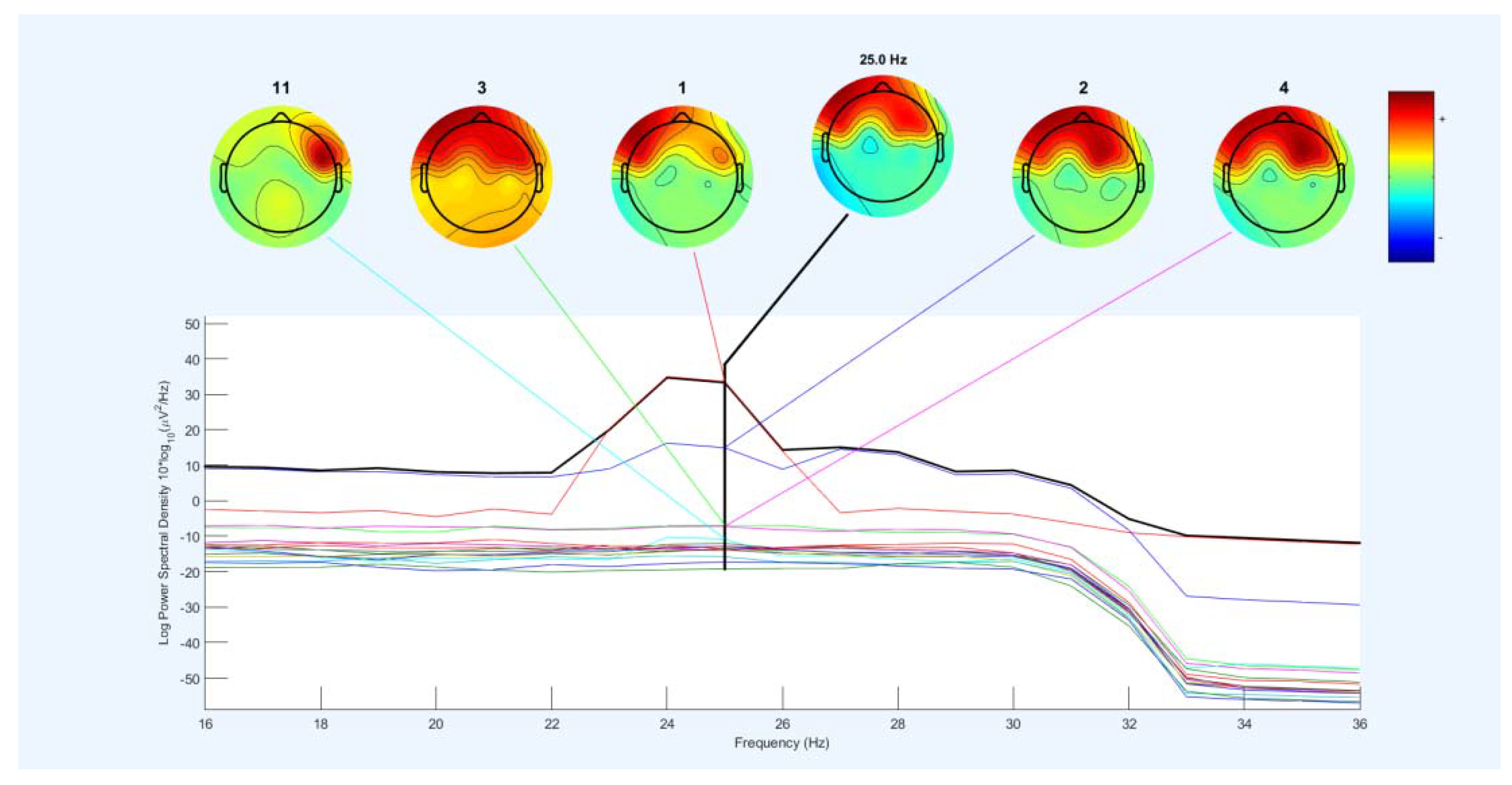
In this paper, the lagrangian polynomial equation is introduced for extracting coefficients as features, which leads to select the best coefficients of formula for increasing performance. The effective distinctive pattern is applied on one or more coefficients. For our experiment, a limited time of about 1second is tested that effective brain function (three channels in front of the brain) is one feature. Due to converting of 0.5 and 1 second of data to formula, it is impossible to describe the main relationships of coefficients with brain activities. It is necessary to examine different brain locations, large-scale frequency domains (8Hz-30Hz), and different times of recording EEG signals to find the relationship of coefficients with order and location relationship of brains and time sizes of brain activities.

5.3. General Discussion About Bond Graph Classifier for suppliment of SVM in noisy signals

This paper introduces a new supplement for the SVM classifier for noisy data. This idea is like a hyper-plane model, which is different from SVM linear model for finding a hyper-plane. When data is very noisy, the classifier does not need to be highly sensitive to find a very well boundary. Our classifier is not very sensitive to finding suitable borders in noisy data. It can increase performance between 2 to 3% accuracy.

5.4. General Discussion About Deep Formula Detection and Extracting Roots Classifier

When compared with QRNN, it is 3% less accurate. Our best results (63.15%) are 3% less accurate than QRNN (66.59%) under the same test conditions. In comparison, f RAW (64.27) has 1% less accuracy. This FBCNN with the same weight can achieve close to this accuracy method with less accuracy.
When compared with CNN models, our proposed idea has 10% lower accuracy than CNN, 7% lower than CNN, 17% lower than DBN, 19% lower than RNN-GRU, and 16% lower Less than RN-LSTM.
In two classes for classification, our proposed method achieved 12% lower accuracy than CNN (Relu, tanh(FC), and sigmoid(FC)), 17% lower than CNN, and 10% lower than CNN. ERlu (conv) and Softmax (FC)).
The essential purpose of the deep neural network is to extract complex features to distinguish patterns to increase accuracy. Therefore, classifiers can obtain the best accuracy and discrimination by using these complex features.
This paper presents a new and different idea for deep learning for the first time, which calls the detection of deep formulaic roots of classes. This model introduces a new model for artificial intelligence and machine learning. With the development of this model, it is possible to provide a model for recognizing deep formulaic roots of activities as formulaic machine learning, which can help the expanse and further understanding of artificial intelligence fields. Because based on the formula, the reasons for the influence of the environment formulas on that formula can examine. But in deep learning, you can’t go into details because they don’t express the layers of information in detail.
The deep formula recognition structure is such that first layer, all electrode or channel data are converted into the formula model. In this article, only one channel uses, but in development, two or more dimensions can uses, but the implementation is somewhat difficult. After the first layer, the processing does on the formula model. Therefore, this paper changes the processing model from the data processing structure to the formula processing structure (the first layer, the data converts into a formula. In the other layers, formulas converts into simple formula. After the extraction in the last layer, formulas are sent to the classifier to extract and identify the roots). Our proposed model needs further research to be excellent, although this model can obtain between 55 and 60% accuracy for a single channel. But it is relatively less accurate. Compared to similar articles for data (except the formula model), there is less difference between them in a single channel. The maximum accuracy for a single channel can be between 60 and 70. One of the reasons that it is less than the others is because it used a frequency range of 4 Hz for processing. The rest uses a 26 Hz frequency for processing. By solving this problem, the accuracy can be increased to between 60 to 70, or high, because most information is lost during the filter to create the bank filter. Other reasons can be related to the following: 1) Choosing a window with the right size to convert data into a formula. 2) Choosing the appropriate sampling size for the coefficients. 3) Select or create a suitable sampling function for the coefficients. 4) Appropriate choice of the frequency range. 5) Choosing the appropriate interval in which the root locates. 6) The selection of long times is used in the first run of one second.
Finally, by developing the proposed method, it is possible to discover the main formula of the complex activity. First, we should seek to recognize the simple activities formula. Then let’s go to the discovery of complex activities formulas. This way can be one of the right ways to solve complex problems. It can explain the hidden part of a system that hides from further understanding. It can introduce different formulas for analysis to find the best ways.

6. Conclusions

Most researchers focus on developing new methods for the future or improving the basic implemented models to identify the optimum standalone feature set. Our research focuses on four ideas. The first introduces future communication models, and the others are improvements of old models or methods. These are: 1) new communication imagery model instead of speech imager using the mental task: Due to speech imagery is very difficult, and it is impossible to imagine sound for all of the characters in all languages. Our research introduces a new mental task model for all the languages that call Lip-sync imagery. This model can use for all the characters in all the languages. This paper implemented two lip-sync for two sounds or letters. 2) New combination Signals: Selecting an inopportune frequency domain can lead to inefficient feature extraction. Therefore, domain selection is so important for processing. This combination of limited frequency ranges proposes a preliminary for creating Fragmentary Continuous frequency. For the first model, two s intervals of 4 Hz as filter banks were examined and tested. The primary purpose is to identify the combination of filter banks with 4Hz (scale of each filter bank) from the 4Hz to 40Hz frequency domain as new combination signals (8Hz) to obtain well and efficient features using increasing distinctive patterns and decreasing similar patterns of brain activities.3) new supplement bond graph classifier for SVM classifier: When SVM linear uses in very noisy, the performance is decreased. But we introduce a new bond graph linear classifier to supplement SVM linear in noisy data. 4) A deep formula recognition model: it converts the data of the first layer into a formula model (formula extraction model). The main goal is to reduce the noise in the subsequent layers for the coefficients of the formulas. The output of the last layer is the coefficients selected by different functions in different layers. Finally, the classifier extracts the root interval of the formulas, and the diagnosis does based on the root interval. The results are between 55% to 98%. Less result is 55% for the deep detection formula, and the highest result is 98% for new combination signals.

Author Contributions

A.N. conceived of ideas. Z. F. helped to complete ideas. A.N. performed the numerical simulations. Z.F. validated the results. A.N. wrote the original draft. Z.F and A.N edit the manuscript.

Funding

This research was funded by National Natural Science Foundation of China, grant number 61876147.

References

  1. Wolpaw, J.R.; Birbaumer, N.; McFarland, D.J.; Pfurtscheller, G.; Vaughan, T.M. Brain–computer interfaces for communication and control. Clin. Neurophysiol. 2002, 113, 767–791. https://www.sciencedirect.com/science/article/pii/S1388245702000573. [CrossRef] [PubMed]
  2. Dornhege, G.; Blankertz, B.; Curio, G.; Müller, K.R. Boosting bit rates in noninvasive EEG single-trial classifications by feature combination and multiclass paradigms IEEE Trans. Biomed. Eng. 2004, 51, 993–1002. https://pubmed.ncbi.nlm.nih.gov/15188870/.
  3. Blankertz, B.; Dornhege, G.; Krauledat, M.; Müller, K.-R.; Curio, G. The non-invasive Berlin Brain–Computer Interface: Fast acquisition of effective performance in untrained subjects. NeuroImage 2007, 37, 539–550. https://www.sciencedirect.com/science/article/pii/S1053811907000535. [CrossRef] [PubMed]
  4. G. Dornhege, J. d. R. Millan, T. Hinterberger, D. J. McFarland, and K.-R. Muller, Eds., Toward Brain-Computer Interfacing. Cambridge, MA: MIT Press, 2007. Available online: https://mitpress.mit.edu/books/toward-brain-computer-interfacing.
  5. Wolpaw, J.R. Brain-computer interfaces as new brain output pathways. J. Physiol. 2007, 579, 613–619. [Google Scholar] [CrossRef] [PubMed]
  6. Gandevia, S.C.; Rothwell, J.C. Knowledge of motor commands and the recruitment of human motoneurons. Brain 1987, 110, 1117–1130. [Google Scholar] [CrossRef]
  7. Blankertz, B.; Losch, F.; Krauledat, M.; Dornhege, G.; Curio, G.; Muller, K.-R. The Berlin Brain-Computer Interface: Accurate performance from first-session in BCI-naive subjects. IEEE Trans. Biomed. Eng. 2008, 55, 2452–2462. [Google Scholar] [CrossRef]
  8. Mensh, B.; Werfel, J.; Seung, H. BCI Competition 2003—Data Set Ia: Combining Gamma-Band Power With Slow Cortical Potentials to Improve Single-Trial Classification of Electroencephalographic Signals. IEEE Trans. Biomed. Eng. 2004, 51, 1052–1056. [Google Scholar] [CrossRef]
  9. Nijboer, F.; Sellers, E.; Mellinger, J.; Jordan, M.; Matuz, T.; Furdea, A.; Halder, S.; Mochty, U.; Krusienski, D.; Vaughan, T.; et al. A P300-based brain–computer interface for people with amyotrophic lateral sclerosis. Clin. Neurophysiol. 2008, 119, 1909–1916. [Google Scholar] [CrossRef]
  10. Panicker, R.; Sadasivan, P.; Sun, Y. Asynchronous P300 Bci: Ssvep-Based Control State Detection. 2011. [Google Scholar] [CrossRef]
  11. Middendorf, M.; McMillan, G.; Calhoun, G.; Jones, K. Brain-computer interfaces based on the steady-state visual-evoked response. IEEE Trans. Rehabilitation Eng. 2000, 8, 211–214. [Google Scholar] [CrossRef]
  12. G. Pfurtscheller, C. Neuper, A. Schlögl, and K. Lugger, Separability of EEG signals recorded during right and left motor imagery using adaptive autoregressive parameters, Rehabilitation Engineering, IEEE Transactions on, vol. 6, pp. 316-325, 1998.
  13. J.M¨uller-Gerking, G. Pfurtscheller, and H. Flyvbjerg, "Designing optimal spatial filters for single-trial EEG classification in a movement task," Clin. Neurophysiol., vol. 110, no. 5, pp. 787–798, 1999. Available online: https://www.sciencedirect.com/science/article/pii/S1388245798000388.
  14. Ramoser, H.; Muller-Gerking, J.; Pfurtscheller, G. Optimal spatial filtering of single trial EEG during imagined hand movement. IEEE Trans. Rehabilitation Eng. 2000, 8, 441–446. https://ieeexplore.ieee.org/document/895946. [CrossRef]
  15. S. Lemm, B. Blankertz, G. Curio, and K.-R.M¨uller, "Spatio-spectral filters for improving the classification of single trial EEG," IEEE Trans. Biomed. Eng., vol. 52, no. 9, pp. 1541–1548, Sep. 2005. Available online: http://citeseerx.ist.psu.edu/viewdoc/summary?doi=10.1.1.61.7985.
  16. Dornhege, G.; Blankertz, B.; Krauledat, M.; Losch, F.; Curio, G.; Müller, K.-R. Combined optimization of spatial and temporal filters for improving brain-computer interfacing. IEEE Trans. Biomed. Eng. 2006, 53, 2274–2281. https://ieeexplore.ieee.org/document/1710169. [CrossRef] [PubMed]
  17. R. Tomioka, G. Dornhege, G. Nolte, B. Blankertz, K. Aihara, and K. R. M¨uller, "Spectrally weighted common spatial pattern algorithm for single trial EEG classification," Dept. Math. Eng., Univ. Tokyo, Tokyo, Japan, Tech. Rep. 40, 2006. Available online: http://doc.ml.tu-berlin.de/bbci/publications/TomDorNolBlaAihMue06.pdf.
  18. W.Wu, X. Gao, B. Hong, and S.Gao, "Classifying single-trial EEG during motor imagery by iterative spatio-spectral patterns learning (ISSPL)," IEEE Trans. Biomed. Eng., vol. 55, no. 6, pp. 1733–1743, Jun. 2008. Available online: https://ieeexplore.ieee.org/document/4457878.
  19. Novi, Q.; Guan, C.; Dat, T.H.; Xue, P. Sub-band common spatial pattern (SBCSP) for brain-computer interface," in Proc. 3rd Int. IEEE/Eng. Med. Biol. Soc. Conf. Neural Eng. 2007; pp. 204–207. [Google Scholar] [CrossRef]
  20. Ang, K.K.; Chin, Z.Y.; Zhang, H.; Guan, C. "Filter bank common spatial pattern (FBCSP) in braincomputer interface," in Proc. 2008 Int. Joint Conf. Neural Netw., 2008; pp. 2390–2397. https://ieeexplore.ieee.org/document/4634130. [CrossRef]
  21. Luo, J.; Feng, Z.; Zhang, J.; Lu, N. Dynamic frequency feature selection based approach for classification of motor imageries. Comput. Biol. Med. 2016, 75, 45–53. [Google Scholar] [CrossRef] [PubMed]
  22. Wei, Q.; Wang, Y.; Lu, Z. "Channel Reduction by Cultural-Based Multi-objective Particle Swarm Optimization Based on Filter Bank in Brain–Computer Interfaces," Unifying Electrical Engineering and Electronics Engineering, Lecture Notes in Electrical Engineering 238, pp 1337-1344, 15 June 2013. [CrossRef]
  23. Chin, Z.Y.; Ang, K.K.; Wang, C.; Guan, C.; Zhang, H. "Multi-class Filter Bank Common Spatial Pattern for Four-Class Motor Imagery BCI," 31st Annual International Conference of the IEEE EMBS Minneapolis, Minnesota, USA, pp. 571-574, September 2-6, 2009. [CrossRef]
  24. Deecke, L.; Engel, M.; Lang, W.; Kornhuber, H.H. Bereitschaftspotential preceding speech after holding breath. Exp. Brain Res. 1986, 65, 219–223. [Google Scholar] [CrossRef]
  25. DaSalla, C.S.; Kambara, H.; Sato, M.; Koike, Y. Single-trial classification of vowel speech imagery using common spatial patterns. Neural Networks 2009, 22, 1334–1339. [Google Scholar] [CrossRef] [PubMed]
  26. L. Wang, X. Zhang and Y. Zhang. Extending motor imagery by speech imagery for brain-computer interface. in: Proceedings of the 35rd Annual Conference of the IEEE Engineering in Medicine and Biology Society, Osaka, Japan, 2013, pp. 7056–7059.
  27. J. W. Brown and R. V. Churchill, "Fourier Series and Boundary Value Problems," McGraw-Hill (5th ed.), New York, 1993.
  28. Stillwell, John (2013). "Logic and the philosophy of mathematics in the nineteenth century". In Ten, C. L. (ed.). Routledge History of Philosophy. Volume VII: The Nineteenth Century. Routledge. p. 204. ISBN 978-1-134-92880-4.
  29. Guerra, E.; de Lara, J.; Malizia, A.; Díaz, P. Supporting user-oriented analysis for multi-view domain-specific visual languages. Inf. Softw. Technol. 2009, 51, 769–84. [Google Scholar] [CrossRef]
  30. oderici G, Shetty S, Leung T, Sukthankar R and Li F F 2014 Large-scale video classification with convolutional neural networks Proc. IEEE Computer Society Conf. Computer Vision Pattern Recognition pp 1725–32.
  31. Graves A, Mohamed A and Hinton G 2013 Speech recognition with deep recurrent neural networks 2013 IEEE Int. Conf. on Acoustics, Speech and Signal Processing pp 6645–9.
  32. Sutskever I, Martens J and Hinton G E 2011 Generating text with recurrent neural networks Proc. of the 28th Int. Conf. on Machine Learning pp 1017–24.
  33. Greenspan, H.; van Ginneken, B.; Summers, R.M. Guest editorial deep learning in medical imaging: overview and future promise of an exciting new technique. IEEE Trans. Med. Imaging 2016, 35, 1153–9. [Google Scholar] [CrossRef]
  34. Jirayucharoensak, S.; Pan-Ngum, S.; Israsena, P.; Jirayucharoensak, S.; Pan-Ngum, S.; Israsena, P. EEG-based emotion recognition using deep learning network with principal component based covariate shift adaptation, EEG-based emotion recognition using deep learning network with principal component based covariate shift adaptation. Sci. World J. 2014, 2014, e627892. [Google Scholar] [CrossRef]
  35. Xu, H.; Plataniotis, K.N. 2016 Affective states classification using EEG and semi-supervised deep learning approaches 2016 IEEE 18th Int. Workshop Multimedia Signal Processing pp 1–6.
  36. Yanagimoto M and Sugimoto C 2016 Recognition of persisting emotional valence from EEG using convolutional neural networks 2016 IEEE 9th Int. Workshop Computational Intelligence Applications pp 27–32.
  37. Qiao, R.; Qing, C.; Zhang, T.; Xing, X.; Xu, X. 2017 A novel deep-learning based framework for multi-subject emotion recognition ICCSS 2017—2017 Int. Conf. Information, Cybernetics and Computational Social Systems pp 181–5.
  38. Salama, E.S.; El-khoribi, R.A.; Shoman, M.E.; Shalaby, M.A.W. EEG-based emotion recognition using 3D convolutional neural networks. Int. J. Adv. Comput. Sci. Appl. 2018, 9, 329–37. [Google Scholar] [CrossRef]
  39. Alhagry S 2017 Emotion recognition based on EEG usingLSTM recurrent neural network Emotion 8 8–11 Tabar Y R and Halici U 2017 A novel deep learning approach for classification of EEG motor imagery signals J. Neural Eng. 14 016003.
  40. Blankertz, B.; Dornhege, G.; Lemm, S.; Krauledat, M.; Curio, G.; Müller, K.-R. The Berlin Brain-Computer Interface: EEG-Based Communication without Subject Training. IEEE Trans. Neural Systems and Rehabilitation Eng. 2006, 14, 147–152. [Google Scholar] [CrossRef]
  41. Lotte, F.; Congedo, M.; Lécuyer, A.; Lamarche, F.; Arnaldi, B. A review of classification algorithms for EEG-based brain–computer interfaces. J. Neural Eng. 2007, 4, R1–R13. [Google Scholar] [CrossRef] [PubMed]
  42. Müller, K.-R.; Krauledat, M.; Dornhege, G.; Curio, G.; Blankertz, B. Machine Learning Techniques for Brain-Computer Interfaces. Biomedical Technology 2004, 49, 11–22. [Google Scholar]
  43. Müller, K.-R.; Tangermann, M.; Dornhege, G.; Krauledat, M.; Curio, G.; Blankertz, B. Machine Learning for Real-Time SingleTrial EEG-Analysis: From Brain-Computer Interfacing to Mental State Monitoring. J. Neuroscience Methods 2008, 167, 82–90. [Google Scholar] [CrossRef] [PubMed]
  44. Anderson, C.W.; Devulapalli, S.V.; Stolz, E.A. Determining Mental State from EEG Signals Using Parallel Implementations of Neural Networks. Sci. Program. 1995, 4, 171–183. [Google Scholar] [CrossRef]
  45. H. Cecotti and A. Gra¨ser, “Time Delay Neural Network with Fourier Transform for Multiple Channel Detection of Steady-State Visual Evoked Potential for Brain-Computer Interfaces,” Proc. European Signal Processing Conf., 2008.
  46. Felzer, T.; Freisieben, B. Analyzing EEG signals using the probability estimating guarded neural classifier. IEEE Trans. Neural Syst. Rehabilitation Eng. 2003, 11, 361–371. [Google Scholar] [CrossRef]
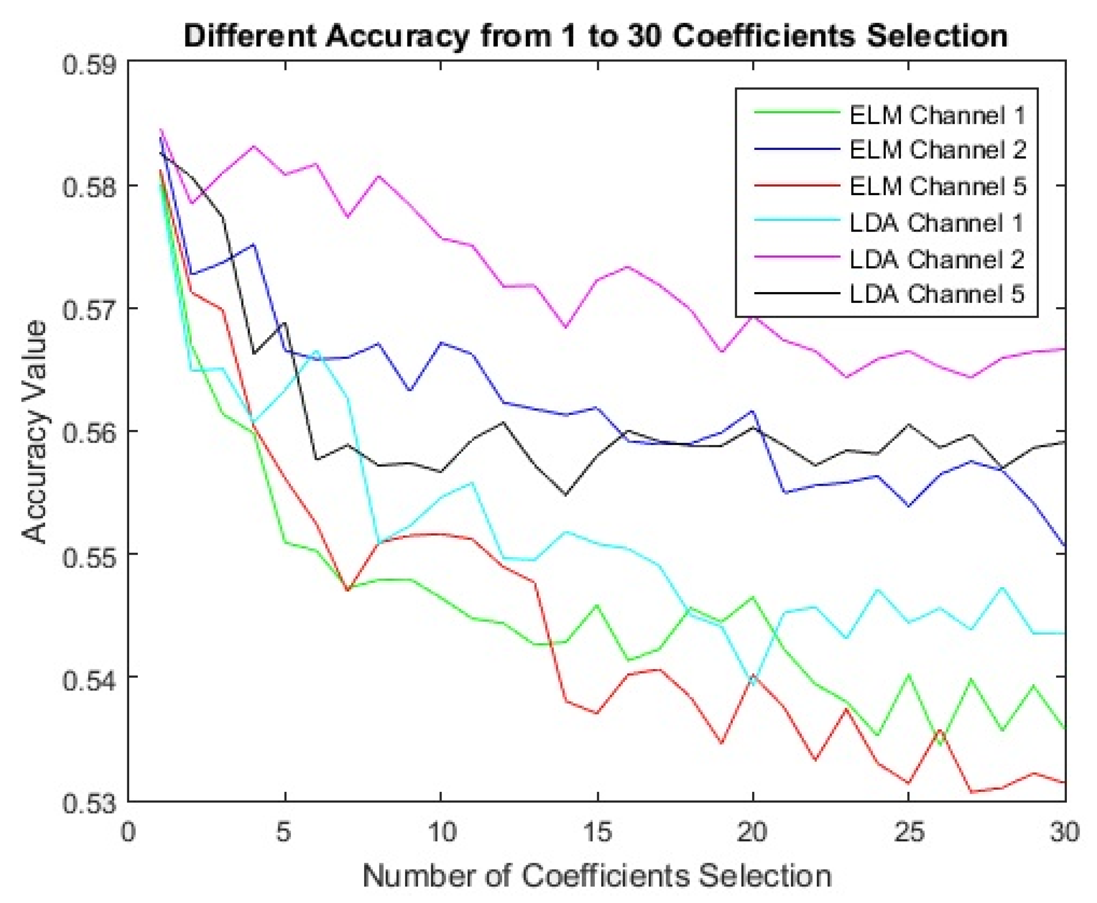
  47. Haselsteiner, E.; Pfurtscheller, G. Using time-dependent neural networks for EEG classification. IEEE Trans. Rehabilitation Eng. 2000, 8, 457–463. [Google Scholar] [CrossRef]
  48. Masic, N.; Pfurtscheller, G. Neural network based classification of single-trial EEG data. Artif. Intell. Med. 1993, 5, 503–513. [Google Scholar] [CrossRef]
  49. Masic, N.; Pfurtscheller, G.; Flotzinger, D. Neural network-based predictions of hand movements using simulated and real EEG data. Neurocomputing 1995, 7, 259–274. [Google Scholar] [CrossRef]
  50. B. Blankertz, G. Curio, and K.-R. Mu¨ller, “Classifying Single Trial EEG: Towards Brain Computer Interfacing,” Advances in Neural Information Processing Systems, T.G. Diettrich, S. Becker, and Z. Ghahramani, eds., vol. 14, pp. 157-164, MIT Press, 2002.
  51. Rakotomamonjy, A.; Guigue, V. BCI Competition III: Data Set II—Ensemble of SVMs for BCI p300 Speller. IEEE Trans. Biomedical Eng. 2008, 55, 1147–1154. [Google Scholar] [CrossRef]
  52. Obermaier, B.; Guger, C.; Neuper, C.; Pfurtscheller, G. Hidden Markov models for online classification of single trial EEG data. Pattern Recognit. Lett. 2001, 22, 1299–1309. [Google Scholar] [CrossRef]
  53. Zhong, S.; Ghosh, J. “HMMs and Coupled HMMs for MultiChannel EEG Classification,” Proc. IEEE Int’l Joint Conf. Neural Networks, vol. 2, pp. 1154-1159, 2002. [CrossRef]
  54. Hiraiwa, A.; Shimohara, K.; Tokunaga, Y. “EEG Topography Recognition by Neural Networks,” IEEE Eng. in Medicine and Biology Magazine, vol. 9, no. 3, pp. 39-42, Sept. 1990. [CrossRef]
  55. Mohamed, A.; Dahl, G.; Hinton, G. , “Deep belief networks for phone recognition,” in Proc. NIPS Workshop Deep Learning for Speech Recognition and Related Applications, 2009.
  56. Mohamed, A.-R.; Dahl, G.E.; Hinton, G. Acoustic Modeling Using Deep Belief Networks. IEEE Trans. Audio, Speech, Lang. Process. 2012, 20, 14–22. [Google Scholar] [CrossRef]
  57. Cireşan, D.C.; Meier, U.; Gambardella, L.M.; Schmidhuber, J. Deep, Big, Simple Neural Nets for Handwritten Digit Recognition. Neural Comput. 2010, 22, 3207–3220. [Google Scholar] [CrossRef]
  58. Hinton, G.E.; Salakhutdinov, R.R. Reducing the Dimensionality of Data with Neural Networks. Science 2006, 313, 504–507. [Google Scholar] [PubMed]
  59. Larochelle, H.; Erhan, D.; Courville, A.; Bergstra, J.; Bengio, Y. An empirical evaluation of deep architectures on problems with many factors of variation. In Proceedings of the 24th International Conference on Machine learning, Corvalis, OR, USA, 20–24 June 2007; pp. 473–480. [Google Scholar]
  60. Hinton, G.E. A practical guide to training restricted Boltzmann machines. In Neural Networks: Tricks of the Trade; Springer: Berlin/Heidelberg, Germany, 2012; pp. 599–619. [Google Scholar]
  61. Hinton, G.E.; Osindero, S.; Teh, Y.-W. A Fast Learning Algorithm for Deep Belief Nets. Neural Comput. 2006, 18, 1527–1554. [Google Scholar] [CrossRef] [PubMed]
  62. Abdel-Hamid, O.; Mohamed, A.; Jiang, H.; Penn, G. Applying Convolutional Neural Networks Concepts to Hybrid NN-HMM Model for Speech Recognition. In Proceedings of the 2012 IEEE International Conference on Acoustics, Speech and Signal Processing (ICASSP), Kyoto, Japan, 25–30 March 2012; pp. 4277–4280. [Google Scholar]
  63. Lee, H.; Pham, P.; Largman, Y.; Ng, A. Unsupervised feature learning for audio classification using convolutional deep belief networks. In Advances in Neural Information Processing Systems 22; Bengio, Y., Schuurmans, D., Lafferty, J., Williams, C.K.I., Culotta, A., Eds.; Cambridge, MA: MIT Press, 2009, pp. 1096–1104. [Google Scholar]
  64. Cecotti, H.; Graser, A. Convolutional Neural Networks for P300 Detection with Application to Brain-Computer Interfaces. IEEE Trans. Pattern Anal. Mach. Intell. 2011, 33, 433–445. [Google Scholar] [CrossRef]
  65. Dahl, G.E.; Yu, D.; Deng, L.; Acero, A. Context-Dependent Pre-Trained Deep Neural Networks for Large-Vocabulary Speech Recognition. IEEE Trans. Audio, Speech, Lang. Process. 2012, 20, 30–42. [Google Scholar] [CrossRef]
  66. Krizhevsky, A.; Sutskever, I.; Hinton, G.E. Imagenet classification with deep convolutional neural networks. Advances in neural information processing systems 2012, 25, 1097–1105. [Google Scholar] [CrossRef]
  67. Mesnil, G.; He, X.; Deng, L.; Bengio, Y. Investigation of recurrent-neural-network architectures and learning methods for spoken language understanding. Interspeech 2013 2013. [Google Scholar] [CrossRef]
  68. Schuster, M.; Paliwal, K. Bidirectional recurrent neural networks. IEEE Trans. Signal Process. 1997, 45, 2673–2681. [Google Scholar] [CrossRef]
  69. Cecotti, H.; Graser, A. Convolutional Neural Networks for P300 Detection with Application to Brain-Computer Interfaces. IEEE Trans. Pattern Anal. Mach. Intell. 2010, 33, 433–445. [Google Scholar] [CrossRef]
  70. Manor, R.; Geva, A.B. Convolutional Neural Network for Multi-Category Rapid Serial Visual Presentation BCI. Front. Comput. Neurosci. 2015, 9, 146. [Google Scholar] [CrossRef]
  71. Liew, A.W.-C.; Leung, S.H.; Lau, W.H. Lip contour extraction from color images using a deformable model. Pattern Recognit. 2002, 35, 2949–2962. [Google Scholar] [CrossRef]
  72. A.J. Goldschen, O.N. Garcia, E.D. Petajan, in: M. Shah, R. Jain (Eds.). Continuous Automatic Speech Recognition by Lipreading, Motion-Based Recognition. Kluwer Academic Publishers, Dordrecht, 1997, pp. 321–343.
  73. R.R. Rao and R.M. Mersereau. Lip modeling for visual speech recognition. Proceedings of the 28th Asilomar Conference on Signals, Systems and Computers, 1994.
  74. A.W.C. Liew, S.H. Leung and W.H. Lau. Lip contour extraction using a deformable model. Proceedings of IEEE International Conference on Image Processing, ICIP-2000, Vancouver, Canada.
  75. G. Rabi and S.W. Lu. Energy minimization for extracting mouth curves in a facial image. Proceedings of IEEE International Conference on Intelligent Information Systems, IIS’97, 1997, pp. 381–385.
  76. Mase, K.; Pentland, A. Lip Reading: Automatic Visual Recognition of Spoken Words. 1989; C1. [Google Scholar] [CrossRef]
  77. W.N. Lie and H.C. Hsieh. Lips detection by morphological image processing. Proceedings of the Fourth International Conference on Signal Processing, ICSP’98, Vol. 2, 1998, pp. 1084–1087.
  78. Michael Vogt. Lip modeling with automatic model state changes. Workshop on Sensor fusion in Neural Networks, SchloW Reisensburg, Germany. 21 July 1996.
  79. S. Basu, A. Pentland. A three-dimensional model of human lip motions trained from video. Proceedings of the IEEE Non-Rigid and Articulated Motion Workshop at CVPR ‘97. San Juan, Puerto Rico, June, 1997.
  80. Jie Wang, Zuren Feng, Na lu,: Feature extraction by Common Spatial Pattern in Frequency Domain for Motor Imagery Tasks Classidication, 2017 29th Chinese Control And Decision Conference (CCDC), ISSN: 1948-9447.
  81. Chen K, Wei Q, Ma Y (2010) An unweigted exhaustive diagonalization based multiclass common spatial pattern algorithm in brain-computer interfaces. In: Proceedings of the 2nd international conference on information engineering and computer science, vol 1, Wuhan, China, pp 206–210. 1.
  82. Ang, K.K.; Chin, Z.Y.; Wang, C.; Guan, C.; Zhang, H. Filter Bank Common Spatial Pattern Algorithm on BCI Competition IV Datasets 2a and 2b. Front. Neurosci. 2012, 6, 39. [Google Scholar] [CrossRef]
  83. Ramoser, H.; Muller-Gerking, J.; Pfurtscheller, G. Optimal spatial filtering of single trial EEG during imagined hand movement. IEEE Trans. Rehabilitation Eng. 2000, 8, 441–446. [Google Scholar] [CrossRef]
  84. Arellano-Valle, R.B.; Contreras-Reyes, J.E.; Genton, M.G. Shannon Entropy and Mutual Information for Multivariate Skew-Elliptical Distributions. Scand. J. Stat. 2013, 40, 42–62. [Google Scholar] [CrossRef]
  85. Contreras-Reyes, J.E. Mutual information matrix based on asymmetric Shannon entropy for nonlinear interactions of time series. Nonlinear Dyn. 2021, 104, 3913–3924. [Google Scholar] [CrossRef]
  86. Goldestein, H. Classical Mechanics, second edition, (Addison-Wesley, 1980).
  87. Walter Gautschi, Numerical Analysis, Second Edition, Library of Congress Control Number: 2011941359. Available online: http://www.ikiu.ac.ir/public-files/profiles/items/090ad_1410599906.pdf. [CrossRef]
  88. Martinez, A. M.; Kak, A. C. (2001). "PCA versus LDA" (PDF). IEEE Transactions on Pattern Analysis and Machine Intelligence. 23 (=2): 228–233.
  89. Abdi. H.& Williams, L.J. (2010). "Principal component analysis". Wiley Interdisciplinary Reviews: Computational Statistics. 2 (4): 433–459. arXiv:1108.4372.
  90. Yang, B.; Tang, J.; Guan, C.; Li, B. Motor Imagery EEG Recognition Based on FBCSP and PCA. 2018. [Google Scholar] [CrossRef]
  91. Rejer, I. EEG Feature Selection for BCI Based on Motor Imaginary Task. Found. Comput. Decis. Sci. 2012, 37, 283–292. [Google Scholar] [CrossRef]
  92. V. Jarník. O jistém problému minimálním [About a certain minimal problem]. Práce Moravské Přírodovědecké Společnosti (in Czech), 6 (4): pp. 57–63, 1930.
  93. Prim, R.C. Shortest Connection Networks And Some Generalizations. Bell Syst. Tech. J. 1957, 36, 1389–1401. [Google Scholar] [CrossRef]
  94. Dijkstra, E.W. A note on two problems in connexion with graphs. Numerische Mathematik 1959, 1, 269–271. [Google Scholar]
  95. Rosen, Kenneth (2011). Discrete Mathematics and Its Applications (7th ed.). McGraw-Hill Science, p. 798.
  96. Cheriton, D.; Tarjan, R.E. Finding Minimum Spanning Trees. SIAM J. Comput. 1976, 5, 724–742. [Google Scholar] [CrossRef]
  97. Naeem, M.; Brunner, C.; Leeb, R.; Graimann, B.; Pfurtscheller, G. Seperability of four-class motor imagery data using independent components analysis. J. Neural Eng. 2006, 3, 208–216. [Google Scholar] [CrossRef] [PubMed]
  98. Dornhege, G.; Blankertz, B.; Curio, G.; Müller, K. Boosting bit rates in noninvasive EEG single-trial classifications by feature combination and multi-class paradigms. IEEE Trans. Biomed. Eng. 2004, 51, 993–1002. [Google Scholar] [CrossRef]
  99. B. Blankertz, K. R. M¨uller, D. J. Krusienski, G. Schalk, J. R. Wolpaw, A. Schl¨ogl, G. Pfurtscheller, J. D. R. M´ıllan, M. Schroder, and N. Birbaumer, “The BCI competition III: Validating alternative approaches to actual BCI problems,” IEEE Trans. Neural Syst. Rehabil., vol. 14, no. 2, pp. 153–159, Jun. 2006.
  100. Clarke, A.R. Excess beta activity in the EEG of children with attention-deficit/hyperactivity disorder: A disorder of arousal? International Journal of Psychophysiology 2013, 89, 314–319. [Google Scholar] [CrossRef]
  101. M. Arvandeh, C. Guan, K.k. Ang and Ch. Quek, "Optimizing the Channel Selection and Classification Accuracy in EEG-Based BCI," IEEE Transaction on Biomedical Engineering, Vol. 58, No. 6, pp 1865-1873, June 2011.
  102. Lotte, F.; Guan, C. Regularizing Common Spatial Patterns to Improve BCI Designs: Unified Theory and New Algorithms. IEEE Trans. Biomed. Eng. 2011, 58, 355–362. [Google Scholar] [CrossRef] [PubMed]
  103. Jin, J.; Xiao, R.; Daly, I.; Miao, Y.; Wang, X.; Cichocki, A. Internal Feature Selection Method of CSP Based on L1-Norm and Dempster–Shafer Theory. IEEE Trans. Neural Networks Learn. Syst. 2020, 32, 4814–4825. [Google Scholar] [CrossRef]
  104. Higashi, H.; Tanaka, T. Simultaneous Design of FIR Filter Banks and Spatial Patterns for EEG Signal Classification. IEEE Trans. Biomed. Eng. 2013, 60, 1100–1110. [Google Scholar] [CrossRef] [PubMed]
Figure 1. Sample of Space-time model of Convolution Neural Network [51].
Preprints 81669 g001
Figure 2. General model of Convolution Neural Network [52].
Preprints 81669 g002
Figure 3. The steps of lip-sync in 2D for M for imagining
Preprints 81669 g003
Figure 4. The steps of lip-sync in 3D for M for imagining
Preprints 81669 g004
Figure 5. The A geometric lip model
Preprints 81669 g005
Figure 6. Feature extraction (FE) from new hybrid signals using common spatial pattern (CSP).
Preprints 81669 g006
Figure 7. Feature selection from the entire set of features extracted from the new signals like FBCSP.
Preprints 81669 g007
Figure 8. Converting data to polynomial formulas and selecting equation coefficients as features with and without selection for classification.
Preprints 81669 g008
Figure 9. Checking of the new hybrid signal by PCA.
Preprints 81669 g009
Figure 10. An overview of the proposed models to run along with the signal combination to generate a new signal from the bank filter.
Preprints 81669 g010
Figure 11. The main structure of connection nodes with distance are described in the left side and prim algorithm find minimum spanning tree in the right side.
Preprints 81669 g011
Figure 12. In the picture, the center of arcs is connected each other of two classes (Blue circle is connected to four around blue circle point of class one. And red center point is also connected to four around red point of class two).
Preprints 81669 g012
Figure 13. There are four state which two center points of two different class need to break to sub tree. This act like recursive algorithm.
Preprints 81669 g013
Figure 14. The step of detection boundary. There are one boundary (a) and two boundaries (b).
Preprints 81669 g014
Figure 15. Creating center point with Arc (radius of circle) based on main tree table.
Preprints 81669 g015
Figure 16. Overview of Formula Pooling Layers look like Data Pooling Layers with normal classifier.
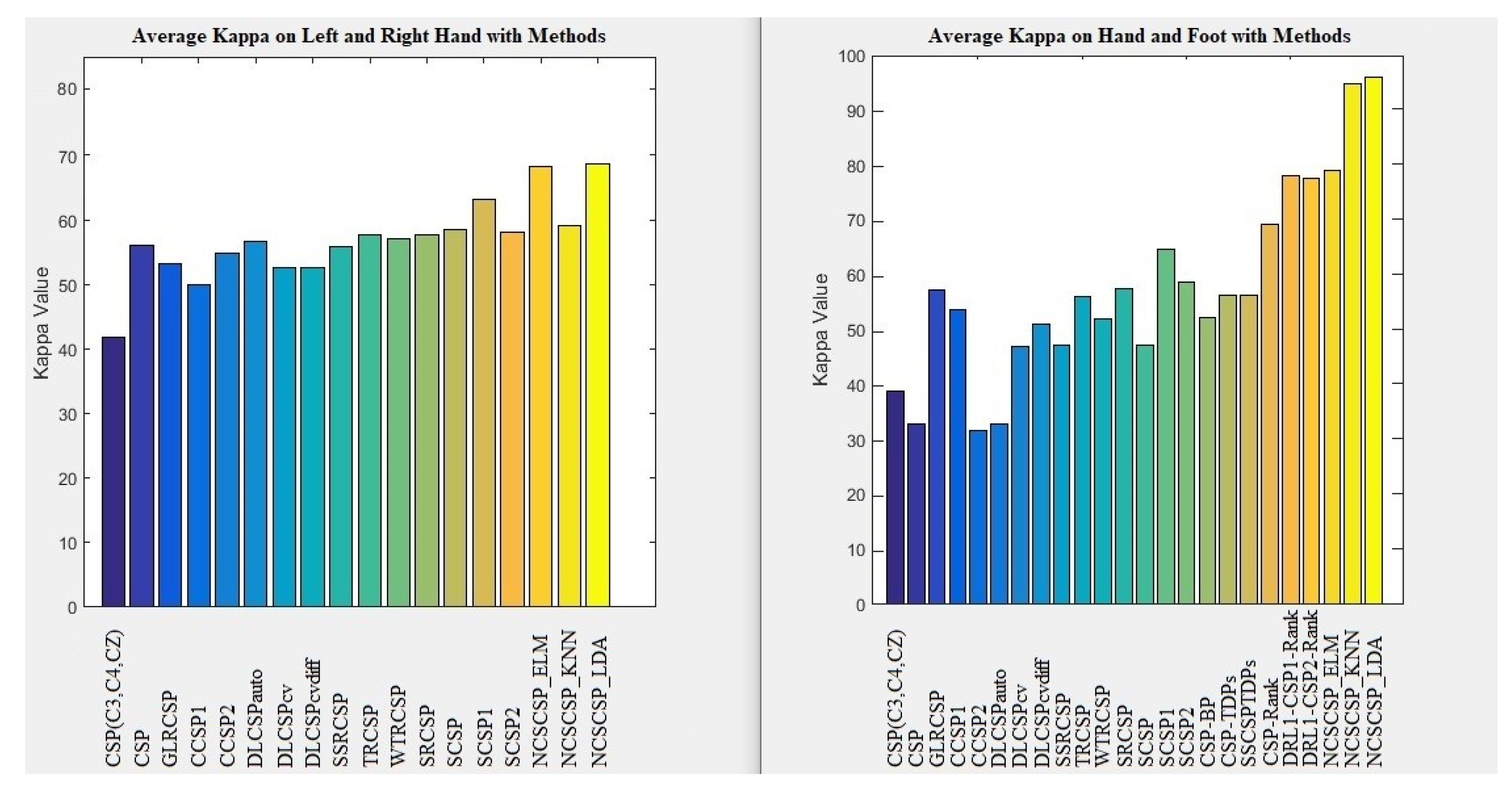
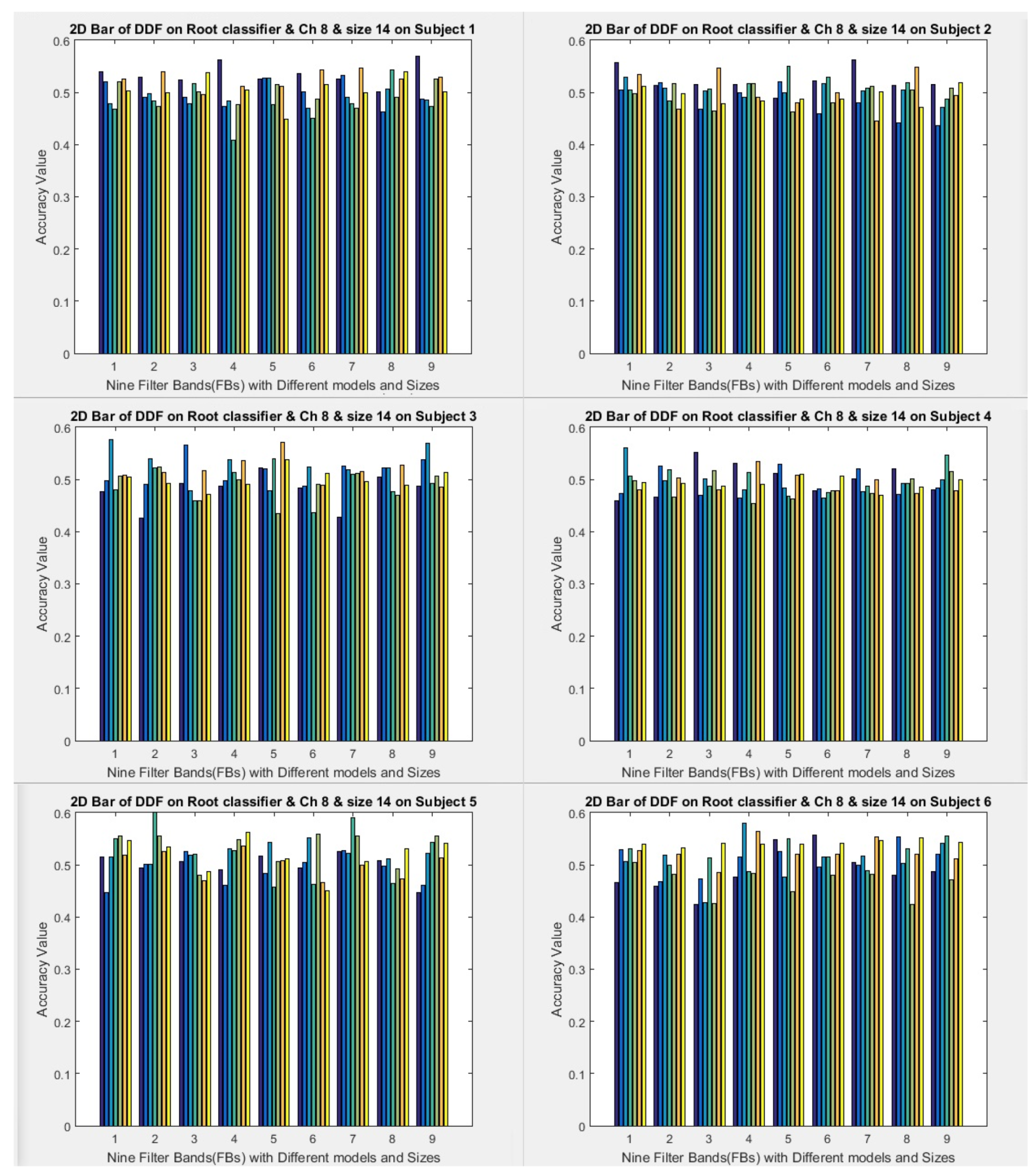
Preprints 81669 g016
Figure 17. Deep Formula Detection with Roots Detection Classifier Structure.
Preprints 81669 g017
Figure 18. Shows eelectrodes montage corresponding to the international 10-20 system.
Preprints 81669 g018
Figure 19. ICA Topography maps on 16 channels between 8-30Hz.
Preprints 81669 g019
Figure 20. maps on power frequency in 25Hz with different channels in between 16-36Hz.
Preprints 81669 g020
Figure 21. Topography maps on power frequency in 25Hz with different channels in between 8-30Hz.
Preprints 81669 g021
Figure 22. Topography maps on power frequency in 25Hz with different channels in between 8-30Hz.
Preprints 81669 g022
Figure 23. Topography maps on power frequency in 25Hz with different channels in between 8-30Hz.
Preprints 81669 g023
Figure 24. ICA Topography maps and power of frequency on the signal channels (C3 and C4) between 2-50Hz.
Preprints 81669 g024
Figure 25. ERSP maps for lip-sync of A and M on channel C3 and C4.
Preprints 81669 g025
Figure 26. ERDS Maps related to lip-sync of M and A in between 23-27Hz
Preprints 81669 g026
Figure 27. Maps of confident Cohen.
Preprints 81669 g027
Figure 28. Accuracy of selected coefficients with ELM and LDA for channels 1, 2, and 5.
Preprints 81669 g028
Figure 29. Left) Evaluation of the best kappa of different methods with new combination signals on the right and left hand. Right) Evaluation of the best kappa of different methods with new combination signals on the hand and foot.
Preprints 81669 g029
Figure 30. Deep Detection on Root classifier on Channel 8 on size 14 on subjects 1 to 6 (Accuracy).
Preprints 81669 g030
Figure 31. Deep Detection on Root classifier on Channel 10 on size 14 on subjects 1 to 6 (Accuracy).
Preprints 81669 g031
Figure 32. Deep Detection on Root classifier on Channel 12 on size 14 on subjects 1 to 6 (Accuracy).
Preprints 81669 g032
Table 1. Classification of all states for 3D lips for A and M.
Subject CSP(m) SVM LDA ELM KNN TREE
S1 4 0.664 0.547 0.634 0.687 0.652
S1 5 0.676 0.582 0.601 0.681 0.658
S2 4 0.624 0.561 0.677 0.619 0.576
S2 5 0.615 0.569 0.698 0.644 0.559
S3 4 0.615 0.571 0.657 0.639 0.546
S3 5 0.632 0.581 0.668 0.664 0.552
Table 2. Average Kappa value of three classifiers using hybrid signals on the left and right hand with 10 features.
Classifier Type FB11&5 FB2&5 FB4&5 FB3&6 FB5&6 FB4&8 FB6&8 FB5&9 FB8&9
ELM 63.31 62.55 63.51 63.19 68.34 63.34 66.92 67.79 62.21
KNN 51.99 50.96 51.81 50.97 59.04 47.95 55.36 56.02 49.57
LDA 64.37 64.31 64.64 61.52 68.70 61.06 64.24 68.22 63.34
1FB I and J means filter bank I and Filter bank J.
Table 3. Kappa value with LDA classifier on hybrid signals on left and right hand with 10 features.
Subject FB11&5 FB2&5 FB4&5 FB3&6 FB5&6 FB4&8 FB6&8 FB5&9 FB8&9
S1 64.08 61.65 66.44 68.87 77.09 56.54 77.75 68.98 68.74
S2 48.44 41.99 47.14 41.97 49.42 40.92 43.46 48.18 50.85
S3 91.37 93.52 88.95 88.81 97.02 75.63 94.42 93.15 70.50
S4 45.61 50.27 51.07 50.30 62.96 60.39 54.11 64.97 58.76
S5 39.20 52.50 46.84 36.95 44.93 47.92 37.44 42.54 50.63
S6 45.36 44.89 59.67 47.49 64.44 48.36 56.97 65.12 51.49
S7 90.60 80.43 59.87 66.65 67.48 63.13 58.43 71.20 68.86
S8 92.01 90.69 95.21 92.61 92.02 91.65 92.23 94.91 88.81
S9 62.64 62.84 66.55 60.02 62.97 65.02 63.41 64.92 61.38
Average 64.37 64.31 64.64 61.52 68.70 61.06 64.24 68.22 63.34
P-value 0.015 0.007 0.004 0.009 0.002 0.014 0.002 0.003 0.016
1FB I and J means filter bank I and Filter bank J. p-value the paired T-test between results of CSP (C3, C4, CZ) [44] and new signals (FB I with J) on the left and right hands.
Table 4. Average sensitivity value of three classifiers using hybrid signals on the left and right hand with 10 features.
Classifier Type FB11&5 FB2&5 FB4&5 FB3&6 FB5&6 FB4&8 FB6&8 FB5&9 FB8&9
ELM_Class_Left 81.65 81.24 82.32 81.89 84.66 81.98 83.78 84.31 81.48
ELM_Class_Rightt 82.85 82.55 82.61 82.56 85.04 82.60 84.26 84.67 82.07
KNN_Class_Left 76.48 76.00 75.95 75.60 80.17 74.18 77.61 78.19 75.18
KNN_Class_Rightt 76.50 75.99 77.02 76.24 80.00 74.79 78.72 78.91 75.61
LDA_Class_Left 81.95 82.23 82.08 81.04 84.09 81.35 82.27 84.15 82.90
LDA_Class_Rightt 83.68 83.42 83.86 81.86 85.97 81.06 83.25 85.44 81.72
1FB I and J means filter bank I and Filter bank J.
Table 5. Average Kappa value of Three classifiers using hybrid signals on hand and foot with 10 features (m=5).
Classifier Type FB11&2 FB4&5 FB4&6 FB4&7 FB4&8 FB1&9 FB2&9 FB3&9 FB4&9
ELM 72.94 73.04 73.41 75.79 75.81 78.36 77.86 78.82 77.93
KNN 91.49 89.63 90.61 94.14 94.10 93.97 94.11 94.60 94.60
LDA 92.47 93.99 93.97 94.50 95.30 95.21 95.77 95.90 95.79
1FB I and J means filter bank I and Filter bank J.
Table 6. Kappa value with LDA classifier on hybrid signals on hand and foot with 10 features (m=5).
Subject FB11&2 FB4&5 FB4&6 FB4&7 FB4&8 FB1&9 FB2&9 FB3&9 FB4&9
S1 94.71 96.57 94.64 95.93 95.79 95.43 95.5 96.42 95.21
S2 92.57 94.64 93.50 94.64 93.64 93.71 94.79 94.04 95.50
S3 86.64 87.71 91.36 92.00 94.86 94.79 95.00 94.78 94.57
S4 92.79 92.71 94.79 95.71 97.86 97.86 97.86 97.86 97.86
S5 95.64 98.29 95.57 94.21 94.36 94.29 95.71 96.38 95.79
Average 92.47 93.99 93.97 94.50 95.30 95.21 95.77 95.90 95.79
P-value 0.0060 0.0053 0.0061 0.0065 0.0067 0.0066 0.0060 0.0061 0.0058
1FB I and J means filter bank I and Filter bank J. P-value the paired T-test between results of CSP (C3, C4, CZ) [44] and new signals (FB I with J) on the left and right hands.
Table 7. Average sensitivity value of Three classifiers using hybrid signals on hand and foot with 10 features.
Classifier Type FB11&2 FB4&5 FB4&6 FB4&7 FB4&8 FB1&9 FB2&9 FB3&9 FB4&9
KNN_Class_Left 88.83 90.18 91.11 91.39 92.18 90.16 92.03 92.72 92.30
KNN_Class_Rightt 89.93 90.28 90.88 91.37 91.88 91.23 92.64 92.32 91.95
LDA_Class_Left 93.48 94.02 93.86 93.81 93.99 94.31 94.15 94.33 94.09
LDA_Class_Rightt 91.90 93.23 93.02 93.36 93.60 93.76 93.99 94.15 94.46
1FB I and J means filter bank I and Filter bank J.
Table 8. Average accuracy on two classifiers based on feature selection (FBCSP) with different umber of features.
Classifier/FS numbers 5 10 15 20 25 30 35 40
LDA_Accuracy 84.05 83.75 83.94 83.96 84.07 83.96 83.91 84.01
KNN_Accuracy 86.51 86.47 86.52 86.52 86.58 86.46 86.55 86.45
LDA_Kappa 68.11 67.49 67.89 67.91 68.13 67.92 67.83 68.01
KNN_Kappa 73.01 72.94 73.04 73.03 73.15 72.92 73.09 72.9
Table 9. Kappa value on KNN classifier based on feature selection (FBCSP) with different number of features.
Subject/ FS numbers 5 10 15 20 25 30 35 40
1 87.12 86.58 87.3 87.35 87.2 86.59 87.12 87.31
2 55.94 55.73 55.8 55.92 55.72 56.52 56.46 55.67
3 92.71 92.63 92.97 92.64 92.68 92.35 92.99 92.49
4 55.81 55.91 55.58 55.66 56.1 55.92 55.58 56.47
5 59.81 59.65 60.11 60.09 60.1 59.39 60.27 59.13
6 59.59 59.34 59.42 59.59 60.26 59.5 59.39 59.05
7 89.5 89.97 90.22 89.73 89.6 89.98 89.65 89.35
8 93.34 93.33 93 93.41 93.55 93.27 93.4 93.64
9 63.31 63.31 62.95 62.89 63.16 62.78 62.98 62.97
Avg 73.01 72.94 73.04 73.03 73.15 72.92 73.09 72.9
Std 16.01 16.06 16.16 16.09 15.97 15.96 16.05 16.12
P_value 0.0039 0.004 0.0041 0.0041 0.0039 0.0042 0.004 0.0039
P-value the paired T-test between results of CSP (C3, C4, CZ) [44] and FBCSP on the different number of features selected.
Table 10. Table 10. Average accuracy on Channel 5 on FBs and 30 selection features with Lagrangian formula.
Classifier-Channel FB14&7 FB1&8 FB4&8 FB7&8 FB1&9 FB2&9 FB5&9 FB7&9 FB8&9
ELM_Channel 5 56.41 57.12 56.80 57.18 58.11 57.39 57.56 57.29 58.16
LDA_Channel 5 57.41 57.35 57.54 58.06 57.98 57.78 58.02 58.25 58.03
1FB I and J means filter bank I and Filter bank J.
Table 11. Classification on Lagrangian formula using feature selection of 1 feature or 30 Features for some channels.
Classifier-FS1-Channel FB11 FB2 FB3 FB4 FB5 FB6 FB7 FB8 FB9
ELM_1FS_channel 1 56.8 58.09 56.7 56.19 57.71 56.78 57.23 56.76 57.71
ELM_30FS_ channel 1 52.17 53.58 52.76 52.89 54.21 52.16 52.72 51.84 53.06
ELM_1FS_ channel 2 54.81 54.52 56.95 58.7 57.28 57.27 55.57 59.71 59.74
ELM_30FS_ channel 2 51.24 53.5 50.44 52.67 51.38 52.87 52.33 51.65 55.33
ELM_1FS_ channel 5 46.08 56.26 55.22 58.69 57.26 56.58 53.47 58.33 55.59
ELM_30FS_ channel 5 47.02 49.71 49.96 54.32 50.91 49.59 51.08 50.23 49.85
LDA_1FS_ channel 1 56.9 57.84 57.45 56.92 57.56 57.5 56.48 57.99 56.53
LDA_30FS_ channel 1 53.36 55.09 55.91 54.66 56.05 56.23 55.18 54.35 54.79
LDA_1FS_ channel 2 58.13 57.19 57.38 57.89 57.56 57.66 56.93 58.45 58.37
LDA_30FS_ channel 2 56.75 55.73 56.32 55.94 56.98 55.24 54.67 56.66 57.11
LDA_1FS_ channel 5 56.87 58.03 58.25 57.56 58.02 57.53 55.84 57.78 57.98
LDA_30FS_ channel 5 52.86 55.82 55.91 53.85 55.35 56 55.62 54.95 53.79
1FS means feature selected. 2FB I means filter bank I.
Table 12. ELM with PCA on Channel 8 and 12 on the left and right hands datasets made by filter banks.
Classifier-Channel-Signal type FB1 FB2 FB3 FB4 FB5 FB6 FB7 FB8 FB9
ELM_ Channel 8_Normal_FB 50.51 50.12 50.4 49.96 50.6 50.28 50.39 50.08 50.08
ELM_ Channel 12_Normal_FB 50.23 50.21 49.48 50.06 49.91 50.33 50.35 50.38 50.2
Table 13. ELM with PCA on Channel 8 and 12 on the left and right hands datasets made by new hybrid signals.
Classifier-Channel-Signal type FB12&3 FB3&4 FB1&5 FB3&7 FB4&8 FB7&8 FB3&9 FB5&9 FB8&9
ELM_Channel 8_New Signal_of_FBs 60.48 58.17 67.87 59.74 63.08 56.70 53.26 63.93 54.98
ELM_ Channel 12_New Signal_of_FBs 60.56 57.44 68.09 59.41 62.86 56.62 52.73 63.64 54.25
1FB I and J means filter bank I and Filter bank J.
Table 14. Evaluation of the best kappa results of different methods with the best accuracy of the average of the combined signals of the filter banks on the right and left hand.
Methods S1 S2 S3 S4 S5 S6 S7 S8 S9 Avg Std P-Value
CSP (C3,C4,CZ) 51.38 6.94 86.1 36.1 6.94 22.22 15.26 73.6 77.76 41.81 29.64 -
CSP 77.78 2.78 93.06 40.28 9.72 43.06 62.5 87.5 87.5 56.02 32.08 0.0125
GLRCSP 72.22 16.66 87.5 34.72 11.12 30.56 62.5 87.5 76.38 53.24 28.48 0.0275
CCSP1 72.22 20.84 87.5 13.88 -1.38 30.56 62.5 87.5 76.38 50 32.2 0.1230
CCSP2 77.78 6.94 94.44 40.28 8.34 36.12 58.34 90.28 80.56 54.79 31.7 0.0125
DLCSPauto 77.78 2.78 93.06 40.28 13.88 43.06 63.88 87.5 87.5 56.64 31.47 0.0105
DLCSPcv 77.78 1.38 93.06 40.28 11.12 25 62.5 87.5 73.62 52.47 32.12 0.0460
DLCSPcvdiff 77.78 1.38 93.06 40.28 11.12 25 62.5 87.5 73.62 52.47 32.12 0.0460
SSRCSP 77.78 6.94 94.44 40.28 12.5 37.5 58.34 94.44 80.56 55.86 31.49 0.0080
TRCSP 77.78 8.34 93.06 41.66 25 34.72 62.5 91.74 83.34 57.57 29.41 0.0050
WTRCSP 77.78 9.72 93.06 40.28 31.94 23.62 62.5 91.66 81.94 56.94 29.52 0.0090
SRCSP 77.78 26.38 93.06 33.34 26.38 27.78 56.94 91.66 84.72 57.56 27.86 0.0035
SCSP 81.94 12.5 93.04 45.82 27.76 27.76 59.72 94.44 83.32 58.48 29.47 0.0030
SCSP1 83.32 34.72 95.82 44.44 30.54 33.34 69.44 94.44 83.32 63.26 25.84 0.0015
SCSP2 83.32 20.82 94.28 41.66 26.38 22.22 56.94 90.26 87.5 58.15 29.44 0.0030
NCSCSP1_ELM 75.95 49.61 94.93 60.76 48.46 61.41 66.2 88.29 69.47 68.34 14.98 0.0260
NCSCSP1_KNN 70.68 29.89 96.65 41.21 38.63 47.18 53.53 87.96 65.63 59.04 21.56 0.0045
NCSCSP1_LDA 77.09 49.42 97.02 62.96 44.93 64.44 67.48 92.02 62.97 68.70 16.46 0.0020
1New Combination Signal with CSP (NCSCSP), and P-value the paired T-test between results of CSP (C3, C4, CZ) [101] and other methods.
Table 15. Evaluation of the best kappa of the results of different methods with the best average accuracy of the combined signals of the filter banks on the hand and foot.
Methods S1 S2 S3 S4 S5 Avg Std P-Value
CSP (C3,C4,CZ) 8.56 60 10 40 74.28 38.57 26.28 -
CSP 32.14 92.86 0 43.76 0 32.56 34.28 0.3850
GLRCSP 44.64 92.86 33.68 35.72 78.58 57.1 24.09 0.0400
CCSP1 33.92 92.86 26.54 43.76 69.84 53.38 24.58 0.0480
CCSP2 30.36 92.86 0 43.76 0 31.4 34.3 0.3635
DLCSPauto 33.92 92.86 0 42.86 0 32.7 34.22 0.3875
DLCSPcv 28.58 92.86 4.08 43.76 65.08 46.86 30.4 0.1780
DLCSPcvdiff 39.28 96.42 10.2 43.76 65.08 50.94 28.69 0.1195
SSRCSP 41.08 92.86 7.14 43.76 50.78 47.12 27.39 0.2370
TRCSP 42.86 92.86 26.54 43.76 73.8 55.96 23.94 0.0365
WTRCSP 39.28 96.42 9.18 43.76 70.64 51.86 29.61 0.0945
SRCSP 44.64 92.86 20.4 55.36 73.02 57.26 24.65 0.0280
SCSP 48.56 88.56 0 54.28 45.7 47.12 28.26 0.2680
SCSP1 61.42 94.28 14.28 70 82.84 64.56 27.51 0.0215
SCSP2 42.84 91.42 14.28 55.7 88.56 58.56 28.97 0.0120
CSP-BP 0 88 36 88 50 52 33.33 0.2145
CSP-TDPs 0 88 38 88 68 56 33.62 0.1140
SSCSPTDPs 34 76 22 62 84 56 23.91 0.0025
CSP-Rank 67.2 95 15 82.2 85.8 69.04 31.83 0.0185
DRL1-CSP1-Rank 72.8 95.8 46.4 85 89.2 77.84 19.47 0.0040
DRL1-CSP2-Rank 70.8 95.8 47.2 85 87.8 77.32 19.11 0.0040
NCSCSP_ELM 80.6 76.5 74.82 80.28 81.88 78.82 2.68 0.0170
NCSCSP_KNN 93.86 94.82 88.04 99.04 97.24 94.60 3.75 0.0050
NCSCSP_LDA 96.42 94.04 94.78 97.86 96.38 95.90 1.35 0.0060
P-value the paired T-test between results of CSP (C3, C4, CZ) [44] and other methods.
Table 16. Evaluation of the best accuracy of the results of different methods with the best average accuracy of the combined signals of the filter banks on the hand and feet.
Methods S1 S2 S3 S4 S5 Avg Std P-Value
CSP (C3,C4,CZ) 54.28 80.00 55.00 70.00 87.14 69.28 14.69 -
CSP-Ref 90.36 98.36 76.64 98.64 94.50 91.70 8.11 0.0049
CSP 81.93 98.64 74.00 97.07 92.86 88.90 9.46 0.0034
CSSP 87.07 95.71 74.86 98.07 94.86 90.11 8.47 0.0039
CSSSP1 90.79 99.11 75.79 99.57 94.21 91.89 8.68 0.0040
CSSSP2 91.00 98.93 76.14 99.07 93.86 91.80 8.41 0.0041
SPEC-CSP 83.93 99.21 72.50 98.93 92.36 89.30 10.11 0.0036
FBCSP1 90.64 98.93 66.29 98.50 96.07 90.09 12.26 0.0035
FBCSP2 89.29 99.07 69.79 98.71 95.64 90.50 10.93 0.0034
FBCSP3 88.21 98.93 72.93 99.00 95.43 90.90 9.81 0.0034
DFBCSP1 92.29 99.29 78.07 99.29 95.07 92.80 7.83 0.0040
DFBCSP2 91.00 99.14 76.43 99.57 95.64 92.36 8.54 0.0037
NCSCSP_ELM 90.30 88.24 87.41 90.14 90.94 89.40 1.34 0.0085
NCSCSP_KNN 96.92 97.40 94.01 99.51 98.62 97.29 1.88 0.0048
NCSCSP_LDA 98.21 97.01 97.39 98.92 98.19 97.94 0.67 0.0054
P-value the paired T-test between results of CSP (C3, C4, CZ) [44] and other methods.
Table 17. Evaluation of the best kappa of the results of different methods with the best average accuracy of the combined signals of the filter banks on the right and left hand.
Methods S1 S2 S3 S4 S5 S6 S7 S8 S9 Avg Std
CSP_Channels 81.94 12.5 93.04 45.82 27.76 27.76 59.72 94.44 83.32 58.48 29.47
CSP 8.55 Channels 83.32 20.82 94.28 41.66 26.38 22.22 56.94 90.26 87.5 58.15 29.44
CSS 13.22 Channels 83.32 34.72 95.82 44.44 30.54 33.34 69.44 94.44 83.32 63.26 25.84
oFBCSP 72 38.9 82.2 38.1 56.3 25.5 80 78.5 74.7 60.7 20.33
sFBCSP 72.1 39.5 81.6 38.4 59.2 28.7 83 78.6 76 61.9 19.94
aFBCSP 74.7 41.6 82.4 40 60.8 30.9 84.9 78.7 77.2 63.5 19.61
NCSCSP1_ELM 75.95 49.61 94.93 60.76 48.46 61.41 66.2 88.29 69.47 68.34 14.98
NCSCSP1_KNN 70.68 29.89 96.65 41.21 38.63 47.18 53.53 87.96 65.63 59.04 21.56
NCSCSP1_LDA 77.09 49.42 97.02 62.96 44.93 64.44 67.48 92.02 62.97 68.70 16.46
1New Combination Signal with CSP
Table 18. Linear Classifier on Dataset SI.
Subject Channel SVM LDA BGL M1 BGL M2 BGL M3
Avg 1 0.501 0.487 0.532 0.535 0.523
2 0.513 0.512 0.517 0.538 0.527
3 0.553 0.652 0.604 0.596 0.554
4 0.558 0.593 0.601 0.61 0.601
Table 19. Non-Linear Classifier on dataset SI.
Subject Channel KNN LDA SVM BG N-Linear
Avg 1 0.579 0.487 0.501 0.553
2 0.595 0.527 0.513 0.554
3 0.657 0.513 0.553 0.56
4 0.623 0.513 0.558 0.561
Table 20. Linear Classifier on Dataset Iva.
Subject Channel SVM LDA BG Linear M1
Avg 1 0.5 0.498 0.498
2 0.539 0.511 0.508
3 0.511 0.498 0.525
4 0.495 0.492 0.502
5 0.515 0.514 0.513
6 0.528 0.514 0.52
7 0.53 0.535 0.518
8 0.519 0.513 0.531
9 0.507 0.497 0.507
10 0.511 0.494 0.505
11 0.515 0.515 0.508
12 0.52 0.517 0.521
13 0.538 0.539 0.545
14 0.507 0.513 0.499
15 0.498 0.487 0.507
16 0.5 0.484 0.519
17 0.502 0.505 0.518
18 0.499 0.504 0.5
19 0.508 0.507 0.499
20 0.515 0.491 0.51
21 0.508 0.502 0.482
22 0.522 0.497 0.504
Table 21. Non-Linear Classifier on Dataset IVa.
Subject Channel KNN TREE BG Non-Linear M1 BG Non-Linear M2
Avg 1 0.518 0.524 0.539 0.492
2 0.495 0.481 0.495 0.498
3 0.506 0.521 0.528 0.492
4 0.493 0.498 0.519 0.511
5 0.485 0.495 0.511 0.498
6 0.527 0.498 0.52 0.516
7 0.495 0.498 0.507 0.495
8 0.504 0.494 0.5 0.495
9 0.533 0.497 0.499 0.51
10 0.51 0.512 0.515 0.495
11 0.503 0.504 0.522 0.498
Table 22. Linear Classifier on Benchmarks Dataset.
Subject SVM LDA BG Linear M1 BG Linear M2 BG Linear M3
Sonar 0.862 0.83 0.826 0.746 0.717
Wisconsin 0.745 0.695 0.674 0.616 0.574
Table 23. Non-Linear Classifier on Benchmark 5 Dataset.
Subject SVM LDA BG Linear M1 KNN TREE
Sonar 0.835 0.789 0.823 0.923 0.835
Wisconsin 0.697 0.653 0.832 0.84 0.697
Iris 0.957 0.861 0.969 0.957 0.957
Table 24. Deep Detection on Root classifier on Channel 8 on size 14 on subjects 7 to 9 (Accuracy).
Subject M-Scale FB1 FB2 FB3 FB4 FB5 FB6 FB7 FB8 FB9
S7 M1-S3 0.478 0.479 0.479 0.489 0.483 0.482 0.469 0.459 0.483
M1-S7 0.51 0.493 0.402 0.497 0.521 0.455 0.489 0.468 0.506
M1-S10 0.506 0.435 0.474 0.41 0.552 0.491 0.474 0.445 0.505
M2-S5 0.486 0.511 0.419 0.506 0.423 0.486 0.518 0.457 0.522
M2-S14 0.48 0.506 0.552 0.458 0.527 0.519 0.503 0.544 0.473
M3-S1 0.488 0.506 0.489 0.493 0.558 0.509 0.482 0.506 0.537
M3-S2 0.473 0.491 0.499 0.486 0.51 0.535 0.496 0.511 0.48
S8 M1-S3 0.552 0.519 0.493 0.506 0.48 0.508 0.512 0.45 0.538
M1-S7 0.487 0.455 0.521 0.492 0.528 0.493 0.524 0.486 0.498
M1-S10 0.468 0.48 0.543 0.476 0.459 0.452 0.498 0.517 0.474
M2-S5 0.546 0.525 0.514 0.491 0.535 0.527 0.507 0.507 0.564
M2-S14 0.522 0.513 0.468 0.52 0.457 0.507 0.524 0.463 0.513
M3-S1 0.517 0.48 0.507 0.477 0.503 0.506 0.482 0.473 0.521
M3-S2 0.479 0.472 0.447 0.46 0.505 0.525 0.469 0.504 0.486
S9 M1-S3 0.476 0.472 0.474 0.455 0.477 0.45 0.498 0.45 0.491
M1-S7 0.513 0.478 0.499 0.473 0.499 0.494 0.516 0.471 0.528
M1-S10 0.53 0.476 0.496 0.52 0.493 0.486 0.477 0.501 0.488
M2-S5 0.531 0.527 0.468 0.499 0.533 0.499 0.52 0.464 0.509
M2-S14 0.466 0.502 0.507 0.471 0.483 0.48 0.501 0.498 0.464
M3-S1 0.546 0.513 0.493 0.559 0.496 0.493 0.475 0.476 0.506
M3-S2 0.496 0.498 0.514 0.479 0.458 0.485 0.502 0.526 0.524
Table 25. Deep Detection on Root classifier on Channel 10 on size 14 on subjects7to 9 (Accuracy).
Subject M-Scale FB1 FB2 FB3 FB4 FB5 FB6 FB7 FB8 FB9
S7 M1-S3 0.444 0.507 0.464 0.51 0.437 0.469 0.514 0.539 0.473
M1-S7 0.517 0.569 0.45 0.518 0.547 0.45 0.523 0.536 0.465
M1-S10 0.507 0.534 0.479 0.59 0.517 0.514 0.544 0.481 0.548
M2-S5 0.439 0.479 0.502 0.413 0.517 0.525 0.493 0.546 0.475
M2-S14 0.522 0.508 0.549 0.518 0.554 0.471 0.51 0.555 0.51
M3-S1 0.491 0.476 0.481 0.46 0.5 0.591 0.489 0.498 0.498
M3-S2 0.516 0.469 0.51 0.477 0.546 0.525 0.476 0.548 0.515
S8 M1-S3 0.557 0.563 0.522 0.573 0.482 0.554 0.575 0.462 0.547
M1-S7 0.479 0.536 0.49 0.473 0.504 0.454 0.45 0.518 0.502
M1-S10 0.502 0.465 0.5 0.485 0.496 0.47 0.467 0.452 0.49
M2-S5 0.524 0.475 0.497 0.487 0.541 0.532 0.508 0.501 0.509
M2-S14 0.512 0.494 0.467 0.495 0.515 0.494 0.49 0.462 0.516
M3-S1 0.5 0.464 0.536 0.466 0.52 0.526 0.433 0.551 0.489
M3-S2 0.509 0.463 0.503 0.473 0.511 0.548 0.486 0.503 0.501
S9 M1-S3 0.442 0.462 0.469 0.496 0.491 0.562 0.429 0.472 0.496
M1-S7 0.508 0.521 0.501 0.541 0.517 0.534 0.502 0.52 0.492
M1-S10 0.486 0.518 0.51 0.489 0.495 0.459 0.479 0.543 0.469
M2-S5 0.536 0.511 0.466 0.552 0.491 0.548 0.531 0.477 0.508
M2-S14 0.464 0.48 0.498 0.497 0.447 0.515 0.471 0.505 0.466
M3-S1 0.52 0.503 0.52 0.539 0.519 0.505 0.504 0.516 0.504
M3-S2 0.474 0.461 0.483 0.47 0.481 0.536 0.475 0.467 0.489
Table 26. Deep Detection on Root classifier on Channel 12 on size 14 on subjects7to 9 (Accuracy).
Subject M-Scale FB1 FB2 FB3 FB4 FB5 FB6 FB7 FB8 FB9
S7 M1-S3 0.486 0.508 0.482 0.473 0.489 0.519 0.475 0.477 0.456
M1-S7 0.484 0.442 0.494 0.488 0.535 0.463 0.533 0.428 0.523
M1-S10 0.5 0.482 0.45 0.456 0.466 0.472 0.516 0.501 0.523
M2-S5 0.576 0.506 0.534 0.512 0.484 0.503 0.52 0.471 0.546
M2-S14 0.448 0.476 0.512 0.479 0.526 0.488 0.458 0.508 0.456
M3-S1 0 0 0 0 0 0 0 0 0
M3-S2 0.526 0.51 0.474 0.517 0.532 0.506 0.507 0.509 0.524
S8 M1-S3 0.533 0.549 0.454 0.544 0.45 0.524 0.553 0.478 0.505
M1-S7 0.49 0.496 0.484 0.45 0.492 0.504 0.483 0.493 0.527
M1-S10 0.468 0.501 0.505 0.446 0.485 0.528 0.488 0.434 0.493
M2-S5 0.476 0.557 0.511 0.49 0.484 0.535 0.541 0.497 0.504
M2-S14 0.491 0.484 0.455 0.502 0.46 0.488 0.492 0.463 0.501
M3-S1 0 0 0 0 0 0 0 0 0
M3-S2 0.488 0.512 0.488 0.521 0.515 0.536 0.515 0.475 0.468
S9 M1-S3 0.53 0.509 0.503 0.509 0.495 0.575 0.506 0.517 0.514
M1-S7 0.535 0.535 0.453 0.555 0.507 0.492 0.521 0.522 0.531
M1-S10 0.488 0.539 0.487 0.42 0.484 0.517 0.5 0.503 0.413
M2-S5 0.48 0.496 0.448 0.472 0.496 0.466 0.494 0.518 0.475
M2-S14 0.488 0.502 0.527 0.51 0.474 0.481 0.514 0.519 0.497
M3-S1 0 0 0 0 0 0 0 0 0
M3-S2 0.508 0.511 0.546 0.51 0.455 0.513 0.522 0.524 0.515
Table 27. All of running of 10-10 Fold of best subject accuracy with 62.08% accuracy.
Run/Fold F1 F2 F3 F4 F5 F6 F7 F8 F9 F10 Avg
R1 0.759 0.643 0.533 0.655 0.607 0.517 0.69 0.552 0.607 0.724 0.629
R2 0.552 0.69 0.483 0.571 0.679 0.552 0.679 0.700 0.607 0.533 0.604
R3 0.733 0.621 0.536 0.536 0.750 0.724 0.655 0.552 0.643 0.633 0.638
R4 0.679 0.536 0.633 0.517 0.621 0.621 0.690 0.500 0.690 0.724 0.621
R5 0.633 0.714 0.655 0.536 0.571 0.655 0.690 0.448 0.633 0.607 0.614
R6 0.571 0.633 0.571 0.724 0.586 0.750 0.500 0.586 0.621 0.633 0.618
R7 0.633 0.500 0.655 0.667 0.517 0.607 0.643 0.786 0.828 0.517 0.635
R8 0.679 0.429 0.600 0.633 0.552 0.621 0.643 0.690 0.724 0.607 0.618
R9 0.655 0.571 0.821 0.467 0.586 0.500 0.655 0.679 0.433 0.724 0.609
R10 0.714 0.621 0.655 0.536 0.517 0.448 0.586 0.655 0.69 0.793 0.622
Table 28. FBCNN on five different models for running and update with PSO.
Subject/Model SVM LDA KNN RF TREE
Train Text Train Text Train Text Train Text Train Text
S1 0.521 0.507 0.59 0.512 1 0.507 0.622 0.485 0.984 0.485
S2 0.542 0.486 0.608 0.535 1 0.521 0.606 0.503 0.983 0.485
S3 0.507 0.500 0.553 0.499 1 0.479 0.639 0.532 0.978 0.499
S4 0.539 0.479 0.548 0.487 1 0.528 0.579 0.524 0.99 0.438
S5 0.521 0.507 0.565 0.526 1 0.479 0.632 0.528 0.983 0.555
Avg 0.521 0.496 0.573 0.512 1 0.503 0.616 0.514 0.983 0.492
Disclaimer/Publisher’s Note: The statements, opinions and data contained in all publications are solely those of the individual author(s) and contributor(s) and not of MDPI and/or the editor(s). MDPI and/or the editor(s) disclaim responsibility for any injury to people or property resulting from any ideas, methods, instructions or products referred to in the content.
Copyright: This open access article is published under a Creative Commons CC BY 4.0 license, which permit the free download, distribution, and reuse, provided that the author and preprint are cited in any reuse.
Prerpints.org logo

Preprints.org is a free preprint server supported by MDPI in Basel, Switzerland.

Subscribe

© 2024 MDPI (Basel, Switzerland) unless otherwise stated