Submitted:
05 August 2023
Posted:
07 August 2023
You are already at the latest version
Abstract
Backgroumd: The feeling of nasal obstruction is one of the most complaints of the Ear Nose and Throats (ENT) patients. The reason of this complaint is variable, such as Nasal Septal Deviation (NSD). NSD is a significant obstacle to normal respiration and the volume of air entering the lungs.
Understanding how the deviation causes the obstruction is so important, because it leads to better management of this disease. Rhinomanometry and acoustic rhinometry are methods that are used for objective evaluation of upper airway, but they are semi invasive and the accuracy are not guaranteed.
With development of Computed Tomography (CT scan) and Computational Fluid Dynamics (CFD), numerical studies on airflow in different parts of the nasal cavity have been performed.
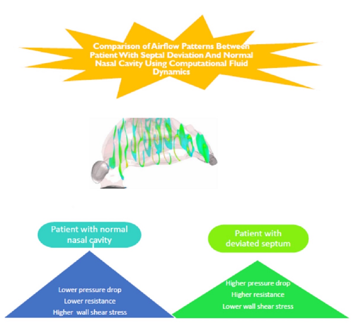
Objectives: The purpose of this study was to compare nasal airflow patterns between patient with NSD and healthy nasal cavity using a computational fluid dynamics (CFD)
Methods: A patient with NSD and a healthy human were selected. Using CFD, the maximal airflow velocity, nasal resistance, maximal Wall Shear Stress (WSS), and pressure drop in bilateral nostrils of both cases were assessed.
Results:
Pressure and velocity profiles are evaluated at a mass flow rate of 17.4 Liters Per Minute (LPM). The velocity profile shows an abnormal flow profile in the septal deviated nasal cavity and the peak velocity is observed at the middle nasal region, whereas this point is at the nasal valve level in a healthy nasal cavity.
Wall shear stress (WSS) caused by NSD is lower than in normal nasal cavities.
The pressure drop in a nasal cavity with deviated septum is higher than in a healthy nasal cavity.
Based on the results of this investigation nasal resistance in NSD was higher than in normal, healthy nasal cavity.
Conclusions: NSD plays an important role in nasal airflow regime and it results in the feeling of obstruction comparing to normal nasal cavity. Also there is a promising future for CFD to become a useful tool in understanding airflow physiology and pathology.
Keywords:
Nasal Septal Deviation (NSD)
; Nasal cavity
; Computational Fluid Dynamics (CFD)
1. Introduction
The nasal cavity is one of the most critical parts of the human respiratory system, which provides the first protection stage of the lungs by heating and moistening the air [1,2,3]. The upper respiratory tract from the valve of the nose to the enterance of the larynx, plays an important role in delivering oxygen to the lungs, thereby absorbing blood. However, the cross-sectional regularity of the air passage from the nasal cavity to the larynx plays a very important role in getting enough oxygen to the lungs and improving respiration. Hence, a better understanding of how stream lines of airflow, the velocity and pressure at obstructive and critical points in the nasal cavity on the inhaled airflow is essential [4,5].
The complicated structure associated with the nasal anatomy makes it difficult for the measurement of nasal resistance [6]. Identifying the influence of nasal anatomy is made difficult by the small size of these airways and the influence of the sensitive mucosa. Several researchers have undertaken studies pertaining to airflow through nasal cavity using measuring devices such rhinomanometer and rhinoacoustic manometry [7,8,9,10].
Harkma et al. and Grotberg reported that determining the exact location of the occlusion in the upper airway is the first step in identifying the critical factors involved in exacerbating nasal and upper airway pathology [11]. Therefore, it is very important to understand the distribution of airflow and obstruction in the human nasal airway. Airflow through the human upper airway has been studied numerically and experimentally by a number of researchers [12,13,14,15,16,17,18,19,20,21,22,23,24,25,26].
Also several researchers have performed studies of airflow through the nasal cavity using measuring devices such as rhinomanometry and acoustic rhinomanometry [27,28,29,30,31].
Rhinomanometry is used to measure the pressure of air flow through the nasal airway and acoustic rhinometry is used to measure the cross section of the airway in different planes of the nose. However, measuring the exact velocity of the airflow and assessing the cross-sectional obstruction in each part of the nasal cavity is difficult [31].
The anatomical complexity of the nasal cavity makes it difficult to measure the amount of obstruction in the nasal cavity. The small size of the nasal cavity and the passage of airflow through it can disrupt the airflow with each probe (rhinomanometric measuring instrument) inserted. Also, the reliability of the result obtained using this device depends on the favorable cooperation of the operator of the rhinomanometric device and the patient, and the calibration of the device and the correct executive instructions by the physician and standard techniques. Due to the inherent limitations of existing measuring instruments, CFD has been proposed as a suitable option [32].
Computational Fluid Dynamics (CFD), which refers to the use of numerical methods to solve the partial differential equation governing fluid flow, is becoming an increasingly popular research tool in the study and prediction of fluid motion [33].
Dmitry Tretiakow et al. used nasal CT scan of 16 patients to image process and model generate of the human nasal cavity and paranasal sinuses using open-source and freeware software. 3-D Slicer for segmentation and new surface model generation. Further processing was done using Autodesk ® Mesh mixer TM. The governing equations were discretized by means of the finite volume method. Subsequently, the corresponding algebraic equation systems were solved by open foam software. The CFD results were presented based on examples of 3-D models of the patient 1 (normal) and patient 2 (pathological changes). As a conclusion CFD is recommended to be used in clinical practice and also in rerearch as a beneficial objective tool to evaluate nasal airway [34].
CFD is also useful in evaluating the outcomes of nasal surgery. For example partial or complete inferior turbinate reduction is assessed and compared in Thomas S et al. study using CFD analysis [35].
The mechanism of feeling obstruction in a patient with atrophic rhinitis using CFD is discussed well in Ya Zhang et al. study [36].
In this study we aimed at using CFD to evaluate upper airway flow characteristics in two nasal cavities one with NSD and the other is normal nasal cavity. Airflow regieme is compared in these two cases in order to clarify the mechanism of feeling obstruction in a patient with NSD.
2. Methods
2.1. Geometry reconstruction:
Two maxillofacial computed tomography (CT) scans from two different subjects were selected for this study. First patient was a 45-year-old Iranian man who suffered from respiratory problems due to right nasal congestion. His NOSE score was 12 (Nose questionnaire is uploaded as supplementary file). Second patient was a 40 year- old Iranian man whose nose was not obstructed and the nasal CT scan was done due to headache. His NOSE score was 3.
None of them have nasal polyposis or past surgery on nose, trauma or common cold over the past month.
The images referenced in this article are 1000 images from all directions input into the Materialize Mimics software (Figure 1 and Figure 2).
CT scans were imported in to medical imaging software (Mimics 19; Materialsize, Plymouth, MI). A three-dimensional reconstruction of the nasal cavity was performed with the exception of the paranasal sinuses which were elongated using a linear tube.
2.2. Mesh generation
Output of Mimics is uncontious and is called .STL (Figure 3). This format does not have the ability to be used in Ansys Meshing and Fluent, so .STL file was driven to the software that is called CATIA, these point clouds converted to line and then model took volume. The surface as well as to smooth and clear the extra points and define the boundary conditions. This format is called .STEP (Figure 4).
Lastly, the .STEP geometry was inputted into the Ansys ICEM CFD program and the calculation grid was produced. Subsequently, through mesh independence analysis, the optimal grid was chosen from a selection of four computational grid models consisting of 3.89, 4.83, 5.67, and 6.53 million mesh components. Among these options, the 6.53 million model was found to be the most suitable (Figure 5).
2.3. Governing equations
2.3.1. Model of Air Flow in Nasal Cavity
In order to simulate the turbulent fluid flow in the incompressible and steady-state conditions for the present air way.
The most successful way of discretising a flow problem is by using the control volume method, also called the finite volume method or Eulerian approach. As the name implies, the problem is divided into control volumes and conservation laws of physics are applied on this volume. The governing equations are
- The continuity equation (conservation of mass)
- The momentum equation (Newton’s second law)
- Reynolds transport theorem
Reynolds transport theorem is applied to the governing equations to transform them into Eulerian form [37].
Conservation of mass Conservation of mass means that the amount of mass stays constant over time. Therefore, if there is mass flow through a volume, then the rate of accumulation within that volume equals the net efllux. In vector notation:
This is also called the continuity equation for a compressible fluid in an unsteady flow. For an incompressible fluid the continuity equation reduces to
2.3.2. Reynolds transport theorem
The rate of change of a general property per unit volume can be expressed in a similar way as the rate of change of mass per unit volume (equation 1)
In words: The rate of change of property _ equals the sum of the rate of increase of in the control volume and the net efflux.
2.3.3. The Momentum Equation
Once Reynolds transport theorem is established, it can be applied to Newton’s second law to calculate the rate of change of momentum using the control volume approach.
Using
The sum of forces on the volume is the sum of pressure, gravity (and other body forces), shear and normal stress forces. [37] Applying Reynolds transport theorem to Newton’s second law on a three-dimensional infinitesimal control volume yields the differential Navier-Stokes equation in three-dimensions for laminar flow [38]:
This case is turbulent, which means there are velocity fluctuations and extra shear stresses to attend to, called Reynolds stresses. Velocity is modeled as the sum of a mean value and a fluctuating value, u=U+u’. A slightly different version of Navier-Stokes emerges
using the Boussinesq approximation for the Reynolds stress (turbulent stress) term on the right side:
yielding, after insertion and rearrangement, the Reynolds-averaged Navier-Stokes equation for turbulent flow [63].
The transient term on the left is of course zero for a steady-state case, leaving the convective term alone on the left side. P represents pressure, k is kinetic energy, and the two remaining terms represent diffusion (turbulent stress) and viscous stresses. is the Kronecker delta, which is necessary for the formula to give the right result for normal Reynolds stresses.
Turbulent kinetic energy equation (k):
Pseudo-vortices equation ()
It is be noted that summation notation i, j = 1, 2, 3 demonstrate the components of the velocity vector and the spatial coordinates. Turbulent viscosity and its formulation are presented in details in Refrence [39]. It is noted that in this study, steady-state condtion is applied, therefore first terms in Equations (6) through (8) are ignored.
2.3.4. Numerical solution
The governing equations combined leave a closed system with an equal number of equations and unknowns. What remains now is a procedure for solving these equations numerically. Ansys Fluent 18’s solver for incompressible steady state turbulent flow is called simple algorithm, and solves the flow using the SIMPLE algorithm.
2.3.5. The SIMPLE Method
SIMPLE, Semi-Implicit Method for Pressure-Linked Equations, starts with a (preferably qualified) guess of initial and boundary conditions for the pressure field. The guessed value is denoted with an asterisk, P*. P* is applied to the discretised momentum equations in order to calculate velocities, These velocities are denoted and treated as guessed values.
The continuity equation is used to express a correction to the pressure, P′. Guessed and correction values are summed to obtain the actual pressure. Similarly, velocity corrections are added to :
After pressure and velocities are corrected, the other discretised transport equations are solved. This concludes one iteration. The process is repeated using the corrected pressure and velocities as initial guesses for the next iteration. This continues until some convergence criterion has been fulfilled. There may be different criteria for different flow properties. Convergence criteria for this thesis are discussed in Section 2.3.7. A flowchart for the SIMPLE method from Versteeg & Malalasekera is shown below [40].
There are several versions of this algorithm, such as the SIMPLE revised or SIMPLER method, which calculates the pressure field directly through a discretized equations for pressure [40]. Nevertheless, only the original SIMPLE method was used for this thesis as it is the foundation for the chosen software solver simple.
2.3.6. Under-relaxation
The SIMPLE method is prone to instabilities. One way to prevent this is by introducing under-relaxation coefficients, , for the pressure and velocity corrections. An under relaxation coefficient is a factor between 0 and 1 that is used to dampen corrected values.
Now, even if the solution oscillates the amplitude is reduced, which may stop the solution from oscillating or diverging. However, this will also lead to slower convergence. The optimum relaxation coefficient in dependent on mesh, flow problem and iteration method and is hard to predict [40].
2.3.7. Numerical schemes
The most important fundamental properties of discretisations schemes are:
- Conservativeness: The amount of a property entering a cell face from one side is the same as the amount leaving the same face on the other side.
- Boundedness: Property value at a point is within the range spanned by its boundaries
Boundary valueMIN < value At Node < boundary valueMax
Transportiveness: The inuence on a cell’s value of a property from its neigbouring cells depends on the relation between convection and diffusion in the flow. This relation is called the Peclet number, Pe. Inuence from a neighbouring cell should be biased according to the Peclet number.
For pure diffusion, -Pe > 0, for pure convection, -Pe > 1
To use an everyday comparison: Shopping for numerical schemes is just like any other shopping: It is difficult to get it all in one product. Desirable characteristics can be mutually exclusive, such as second-order accuracy and boundedness. Also, quality costs. Sometimes the best is simply too expensive, in this context meaning that the time of computation cannot be afforded. That being said, a scheme can perform well enough as long as it suits the problem in question, even if it is only first-order accurate or has poor transportiveness. For instance, the central differencing scheme is adequate for a pure diffusion case, but has poor transportiveness when Pe increases [40]. The schemes in this case a chosen to try to reach second-order accuracy.
2.4. Boundary Conditions
The creation of physical or computational models requires the identification of the boundaries and setting the appropriate values for them. Air ways in nasal cavities have boundaries those are varies with time and usually covered with a thin layer of mucus. Also external shape of the nose affects the internal flow due to inspiration cycle and flow entering the nares. In breathing cycle, airways below the nasopharynx is impressed. Due to mentioned complexity and according to the authors knowledge there is no model has been attempted to cover all these features yet. In the present work, three different con stant flow entrance velocities of 15, 17.4 and 20 LPM are used as an inlet condition to simulate the usual breathing occurring during sleeping, resting, and relaxed situ tions. Also, atmospheric pressure condition is set at the outlet. As mentioned before gravitational acceleration effect is ignored and noslip condition is used on the model walls.
Initial values for k and ω at the inlet are determined using the following relations [41].
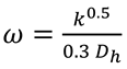 where is the hydraulic diameter and I is the turbulence intensity obtained from following equations [40].
The nasal wall is considered rigid and non-slip [31,42]. A mass flow rate is applied to the nostril inlet, which corresponds to a specific air inlet (liters/minute). The flow range considered in this study ranges 15, 17.4 and 20 LPM and exists in laminar and turbulent regimes for both cases [9,43,44]. As a general rule, for an adult nasal cavity, flow below 15 LPM is considered laminar, between 15 and 17.4 LPM is transient, and above 17.4 LPM is turbulent. For the nasopharynx, the boundary condition “outflow” is considered, which assumes a fully developed flow. This simulation does not take into account the presence of mucus layers and nose hairs. The physical characteristics of the liquid (air) used in this calculation are density of 1.225and kinematic viscosity of 1.7894 × .
The governing equations are discretized over the control volume. Integrating these discretized equations yields a number of equations in algebraic form. Simulations were performed using the CFD solver ANSYS FLUENT 18 R2. The SIMPLE algorithm was chosen to correlate velocity and pressure corrections. For higher accuracy, Second order schemes of momentum, turbulent kinetic energy, and specific dissipation factor are used, and a convergence criterion of four orders of magnitude is adopted.
2.5 Solution Methods
In this study Fluent 18 is applied and convergence criteria is . Solution algo rithms are shown in Figure 6.
3. Results
For better understanding of airflow at different locations and compare changes in area, the nasal cavity is marked with different planes from which values can be extracted, as depicted in Figure 7.
Patterns of airflow in the patient with NSD are described in narrow side. The smallest cross – sectional area in the case of NSD was at the level of 4 cm from nasal tip and this area was 2 cm2, while in normal nasal cavity the smallest cross – sectional area was in 0.5 cm from nasal tip and this area was 2.6 cm2 (Figure 8).
3.1. Velocity and Streamline Contours
The most deviant part of the nasal septum caused the fact that for the septal deviated nasal cavity, the peak velocity was observed in the mid-nasal region on narrow side, while maximum velocity was located at the nasal valve region for the healthy nasal cavity. Velocity contours at the level of 32 mili- meters from nasal tip is shown in Figure 9. (Other Velocity contours are uploaded as supplementary data).
3.2. Pressure Profiles:
Figure 10 shows pressure distribution in NSD and normal nasal cavity in the flow rate of 17.4 LPM. The results reveal that the pressure drop in the case with NSD is more than normal nasal cavity.
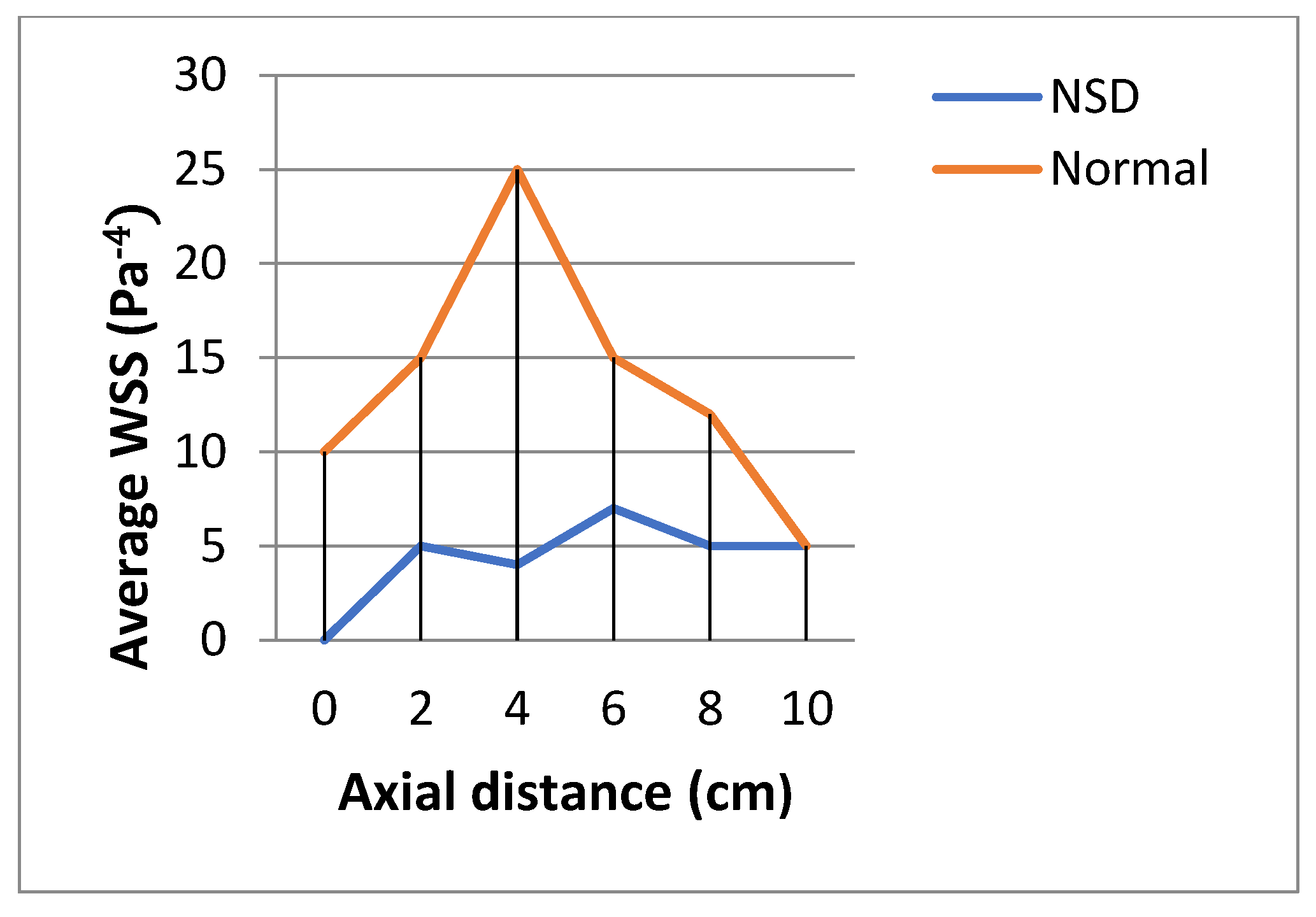
3.3. Wall Shear Stress (WSS)
The wall shear stress showed a peak value along the anterior regions of the inferior turbinate in both cases. WSS was higher in patient without NSD. Figure 11 shows WSS in both cases in the flow rate of 17.4 LPM.
3.4. Resistance
To calculate the resistance R for the patients under study, we used the formula of Zhu et al. [45,46]:
where P is the pressure difference between the nostrils and nasopharynx and Q is the volume flow through the nasal cavity.
According to above equation, resistance in NSD and normal nasal cavity were 0.071 and 0.056 respectively.
4. Discussion
NSD is one of the most frequently etiologies of nasal airway blockage. A deviated septum playing role on the nasal physiology [47]. Complex anatomy of the upper airway caused the fact that many researchers show interest in objective methods for investigating the upper aiway and planning surgeries for nasal pathologies.
Hariri.A. et al. studied relationship between CFD and rhinomanometry results in septoplasty. They found while CFD-derived pressure drops tend to correlate well with preoperative rhinomanometry results, CFD may be better able to detect specific obstruction locations and post-surgical improvements [48].
Dmitry Tretiakow. at al discuss various current and potential applications of CFD in otolaryngology, including evaluating nasal airway abnormalities and surgical interventions. They also note limitations in current modeling approaches [34].
A review by Springett K. et al. discusses how integrating CFD modeling with 3D printing and virtual anatomy tools has the potential to enable highly personalized, evidence-based surgical planning for abnormalities like septal deviations [49].
One of the diseases that affects the nasal cavity is the perforation of the nasal septum, which has various causes, the main causes of which are trauma or systemic diseases. Considering that the method and effect of various treatments are challenge for specialists some researchers such as Wen J. et al. and Kimbell JS. Et al applied CFD models for answering questions about this pathology [50,51].
The treatment of nasal obstruction due to NSD is another challenge which CFD could help to choose the best treatment, for example nasal turbinoplasty, or reduction of the inferior turbinates, is a procedure sometimes performed in patients with nasal obstruction. Turbinate reduction aims to improve nasal airflow by decreasing the size of the turbinates. CFD studies have shown that nasal turbinoplasty can increase nasal airflow, reduce nasal resistance and improve temperature and humidity regulation in the nasal cavity [52].
At this section of the discussion, it is better to mention that the assumption modeling based on CFD often considers the flow to be incompressible and the walls to be rigid, which are actually inherent uncertainties. Also comparisons to normative values should be interpreted cautiously due to differences in methods and sample characteristics.
Considering the above points, in our study velocity shows an unusual velocity distribution pattern in patient with NSD, which is different from normal nasal cavity where a maximum velocity is located at the nasal valve area. The nasal valve area is the narrowest part of the nasal cavity, causing air to accelerate and resulting in the highest velocity. According to the study by Croce et al. and our own study, there is a sudden increase in the cross-sectional area after the nasal valve, leading to a decrease in velocity. The nasal cavity with NSD experiences peak velocities in the middle nasal region and the nasopharynx region, indicating an abnormal flow pattern. This could potentially affect the thermal conditioning and filtration capabilities of the nasal cavity [53].
Pressure drop is traditionally used to validate CFD solutions, measuring the pressure difference between the nostril entrance and the nasopharyngeal exit [51]. According to a study by Ottaviano and Fokkens, pressure drop is thought to have a significant impact on nasal patency [54]. In our study, we observed higher values of pressure drop in nasal cavities with septal deviation compared to healthy nares. This issue is in agreement with previous studies [49,53].
Cevenini G. et al. also reported higher pressure drops and flow abnormalities in deviated septum cavities, reinforcing the potential for CFD modeling to explain nasal obstruction complaints in these patients [56].
WSS is the resistance force that is produced when the air flows within the nasal passage, allowing for the exchange of heat and moisture between the air and the nasal passage. Concentrated levels of these pressures could lead to the inflammation of blood vessels [22].
Our study shows normal nasal cavity leads to higher WSS than the case of NSD. This fact is because of boundary layer production in normal nasal cavity, but in narrowed cavity boundary layer is not produced or partial, since the flow is transient to turbulence. Hence we consider the solve basis on Transient ( method.
WSS and the location where the WSS is the highest is discussed well in Corda et al. study [54]. Their results show nasal valve is where WSS is the highest. In general their findings are similar to our results which is the general trend observed.
A study by Croce A. et al. compares WSS, velocity profiles and pressure drop in normal and deviated septum cavities, finding significant differences which align with the present study’s results [55]. While mean WSS tends to be higher in normal cavities, local WSS maxima may still occur near turbinates in deviated airways. More detailed analyses of WSS distribution patterns are warranted.
Resistance indicates comparatively higher values in a septal deviated nasal cavity when compared to a healthy nasal cavity.
Resistance in healthy adult nasal cavity has been studied in previous studies. Wen et al.[22], Zubair et al. [60] and Weinhold and Mlynski [61] reported the normal nasal cavity resistance at 20 LPM 0.054, 0.06 and 0.068 respectively. Resistance was 0.071 in NSD model according to our study which is higher than normal nasal cavity and it is in agreement with previous studies. The feeling of obstruction can be clarified in NSD, because resistance is higher than normal nasal cavity. While many studies report higher resistance in deviated airways, not all do. Further research is needed to clarify which patient- and septum-specific factors most impact resistance.
This study also has limitations and suggestions for future studies which are numbered below:
- In this study, two nasal cavities of Iranians are considered. This study can be further improvised by including different facial races and more samples.
- Examining seasonal effects and changes due to inflammation or medicated states could be considered in future studies.
- Future studies could be designed by modeling the impacts of surgery or endoscopic treatments on airflow and pressures.
- Investigating interactions between septal deviations and other nasal abnormalities is an interesting topic for further studies.
- The nasal septum plays an important role in nasal physiology, respiratory health, and potentially migraine headaches. Deviations and abnormalities in the nasal septum have been linked to an increased risk of migraine. Researchers hypothesize that nasal septal impairments may contribute to migraines by disrupting factors like nasal airflow, olfaction and inflammatory response that are implicated in migraine pathophysiology [62]. However, further high-quality studies are needed to clarify the mechanisms and establish a definitive causal connection between nasal septal abnormalities and migraines.
- The nasal septum is continuous with the walls of the eustachian tubes, which connect the middle ear cavity to the nasopharynx. Septal abnormalities have been associated with ear infections and eustachian tube dysfunction [63]. Designing studies to investigate this topic using CFD helps ENT surgeons to have comprehensive opinion about ear infections and treat them better.
At last but not least, although septal deviations are common, their impacts vary widely. Patients often perceive obstruction for complex reasons beyond CFD metrics. While CFD insights may inform treatment decisions, they cannot replace in vivo functional diagnostics and patient-reported outcomes. Future research will include the application of CFD in evaluating and comparing medications and surgeries in patients with NSD.
5. Conclusion
Septal deviation, a major cause of nasal obstruction, is assessed in NSD patient and compared to normal nasal cavity. In this study, CT scans of a patient with NSD and a patient normal nasal cavity were used to create a three dimensional model and perform airflow analysis at ranges of 15, 17.4, and 20 LPM.
The narrowest area in NSD is in the middle of the nose, but in normal nasal cavity this area is at the nasal valve.
Velocity patterns show peak nasal velocities at middle nasal cavity in NSD which affect nasal physiological functions.
NSD showed higher nasal resistance compared with healthy nasal cavity. Pressure drop values were higher in nasal cavities with septal deviation than in normal nasal cavity. Therefore, it can be concluded that nasal obstruction with septal deviation should be effectively treated by appropriate nasal interventions that corrects airways and allow smooth airflow.
References
- Hansen F, Wood DE (2013) The adrenal fatigue solution. https://adrenalfa tiguesolution.com/. Accessed 9 Apr 2021.
- Marks TN, Maddux SD, Butaric LN, Franciscus RG (2019) Climatic adaptation in human inferior nasal turbinate morphology: evidence from Arctic and equatorial populations. Am J Phys Anthropol 169(3):498–512 https://doi.org/10.1002/ajpa.23840. [CrossRef]
- Pirila T, Tikanto J. Middle turbinate lateralization for treatment of nasal septal deviation. Laryngoscope. 2017;127(5):1208-12. doi:10.1002/lary.26360. [CrossRef]
- Fettman, N., Sanford, T., and Sindwani, R. (2009). Surgical management of the deviated septum: techniques in septoplasty. Otolaryngol. Clin. North Am. 42, 241–252. https://doi.org/10.1016/j.otc.2009.01.005. [CrossRef]
- Deviated Septum (2021). American academy of otolaryngology-head and neck surgery. https://www.entnet.org/content/deviated-septum-overview.
- Rahimi-Gorji, M., Pourmehran, O., Gorgi- Bandpy, M. (2015). Journal of Molecular Liquids. 209, 121-123.
- Kim SK, Na Y, Kim JI, Chung SK (2013) Patient specific CFD models of nasal airflow: overview of methods and challenges. J Biomech 46(2):299–306 https://doi.org/10.1016/j.jbiomech.2012.1.022. [CrossRef]
- Bruening J, Goubergrits L, Hildebrandt T (2016) Team 190: CFD simulation of airflow within a nasal cavity The UberCloud. https://community.theubercloud.com/wpcontent/uploads/2016/09/Team-190-JanBruening.pdf. Accessed 9 Apr 2021.
- Garcia GJM, Bailie N, Martins DA, Kimbell JS (2007) Atrophic rhinitis: a CFD study of air conditioning in the nasal cavity. J Appl Physiol 103(3):1082– 1092 https://doi.org/10.1152/japplphysiol.0111.2006. [CrossRef]
- Faramarzi M, Baradaranfar MH, Abouali O, Atighechi S, Ahmadi G, Farhadi P et al. (2014) Numerical investigation of the flow field in realistic nasal septal perforation geometry. Allergy Rhinol (Providence) 5(2):70–77 https://doi. org/10.2500/ar.2014.5.0090. [CrossRef]
- Harkema, J. R., Carey, S. a, & Wagner, J. G. (2006). The nose revisited: a brief review of the comparative structure, function, and toxicologic pathology of the nasal epithelium. Toxicologic Pathology, 34(3), 252–269. http://doi.org/10.1080/01926230600713475. [CrossRef]
- Kim, S. K., & Chung, S. K. (2004). An investigation on airflow in disordered nasal cavity and its corrected models by tomographic PIV. Measurement Science and Technology, 15(6), 1090–1096. http://doi.org/10.1088/09570233/15/6/007. [CrossRef]
- Kim, S. K., Na, Y., Kim, J. I., & Chung, S. K. (2013). Patient specific CFD models of nasal airflow: Overview of methods and challenges. Journal of Biomechanics, 46(2), 299–306. http://doi.org/10.1016/j.jbiomech.2012.11.022. [CrossRef]
- Mylavarapu, G., Mihaescu, M., Fuchs, L., Papatziamos, G., & Gutmark, E. (2013). Planning human upper airway surgery using computational fluid dynamics. Journal of Biomechanics, 46(12), 1979–86. http://doi.org/10.1016/j.jbiomech.2013.06.016. [CrossRef]
- Mylavarapu, G., Murugappan, S., Mihaescu, M., Kalra, M., Khosla, S., & Gutmark, E. (2009a). Validation of computational fluid dynamics methodology used for human upper airway flow simulations. Journal of Biomechanics, 42(10), 1553–1559. http://doi.org/10.1016/j.jbiomech.2009.03035. [CrossRef]
- Mylavarapu, G., Murugappan, S., Mihaescu, M., Kalra, M., Khosla, S., & Gutmark, E. (2009b). Validation of computational fluid dynamics methodology used for human upper airway flow simulations. Journal of Biomechanics, 42(10), 1553–1559. http://doi.org/10.1016/j.jbiomech.2009.03.035. [CrossRef]
- Segal, R. A., Kepler, G. M., & Kimbell, J. S. (2008). Effects of differences in nasal anatomy on airflow distribution: A comparison of four individuals at rest. Annals of Biomedical Engineering, 36(11), 1870–1882. http://doi.org/10.1007/s10439-008-9556-2. [CrossRef]
- Weinhold, I., & Mlynski, G. (2004). Numerical simulation of airflow in the human nose. European Archives of Oto Rhino-Laryngology, 261(8), 452–455. http://doi.org/10.1007/s00405-003-0675-y. [CrossRef]
- Wang, S. M., Inthavong, K., Wen, J., Tu, J. Y., & Xue, C. L. (2009). Comparison of micron- and nanoparticle deposition patterns in a realistic human nasal cavity. Respiratory Physiology and Neurobiology, 166(3), 142–151. http://doi.org/10.1016/j.resp.2009.02.014. [CrossRef]
- Wang, Y., Wang, J., Liu, Y., Yu, S., Sun, X., Li, S., … Zhao, W. (2012). Fluid–structure interaction modeling of upper airways before and after nasal surgery for obstructive sleep apnea. International Journal for Numerical Methods in Biomedical Engineering, 28, 528–546. http://doi.org/10.1002/cnm. [CrossRef]
- Wang, Z., Hopke, P. K., Ahmadi, G., Cheng, Y. S., & Baron, P. a. (2008). Fibrous particle deposition in human nasal passage: The influence of particle length, flow rate, and geometry of nasal airway. Journal of Aerosol Science, 39(12), 1040–1054. http://doi.org/10.1016/j.jaerosci.2008.07.008. [CrossRef]
- Wen, J., Inthavong, K., Tian, Z., Tu, J., Xue, C., & Li, C. (2007). Airflow patterns in both sides of a realistic human nasal cavity for laminar and turbulent conditions. 16th Australasian Fluid Mechanics Conference (AFMC), (December), 68–74. Retrieved from http://espace.library.uq.edu.au/view/UQ:132285.
- Wen, J., Inthavong, K., Tu, J., & Wang, S. (2008). Numerical simulations for detailed airflow dynamics in a human nasal cavity. Respiratory Physiology & Neurobiology, 161(2), 125–135. http://doi.org/10.1016/j.resp.2008.01.012. [CrossRef]
- Xiong, G.-X., Zhan, J.-M., Zuo, K.-J., Rong, L.-W., Li, J.-F., & Xu, G. (2011). Use of computational fluid dynamics to study the influence of the uncinate process on nasal airflow. The Journal of Laryngology & Otology, 125(1), 30–37. http://doi.org/10.1017/S002221511000191X. [CrossRef]
- Xiong, G., Zhan, J.-M., Jiang, H.-Y., Li, J.-F., Rong, L.-W., & Xu, G. (2008). Computational fluid dynamics simulation of airflow in the normal nasal cavity and paranasal sinuses. American Journal of Rhinology, 22(5), 477–482. http://doi.org/10.2500/ajr.2008.22.3211. [CrossRef]
- Hilberg, O., Jackson, A. C., Swift, D. L., & Pedersen, O. F. (1989). Acoustic rhinometry: evaluation of nasal cavity geometry by acoustic reflection. Journal of Applied Physiology (Bethesda, Md.: 1985), 66(1), 295–303.
- Jones, A. S., & Lancer, J. M. (1987). Rhinomanometry. Clinical Otolaryngology & Allied Sciences, 12(3), 233–236. http://doi.org/10.1111/j.1365-2273.1987.tb00193.x. [CrossRef]
- Shelton, D. M., & Eiser, N. M. (1992). Evaluation of active anterior and posterior rhinomanometry in normal subjects. Clinical Otolaryngology & Allied Sciences, 17(2), 178–182. http://doi.org/10.1111/j.1365-2273.1992.tb01068.x. [CrossRef]
- Sipila, J., & Suonpaa, J. (1997). A prospective study using rhinomanometry and patient clinical satisfaction to determine if objective measurements of nasal airway resistance can improve the quality of septoplasty. European Archives of Oto-Rhino-Laryngology: Official Journal of the European Federation of Oto-Rhino-Laryngological Societies (EUFOS): Affiliated with the German Society for Oto-Rhino-Laryngology - Head and Neck Surgery, 254(8), 387–390.
- Suzina, A. H., Hamzah, M., & Samsudin, A. R. (2003). Active anterior rhinomanometry analysis in normal adult Malays. The Journal of Laryngology and Otology, 117(8), 605–608. http://doi.org/10.1258/002221503768199924. [CrossRef]
- Ishikawa, S., Nakayama, T., Watanabe, M., & Matsuzawa, T. (2009). Flow Mechanisms in the Human Olfactory Groove. Archives of Otolaryngology--Head & Neck Surgery, 135(2), 156–162. http://doi.org/10.1001/archoto.2008.530. [CrossRef]
- Doorly, D. J., Taylor, D. J., and Schroter, R. C. (2008). Mechanics of airflow in the human nasal airways. Respir. Physiology Neurobiol. 163, 100–110. https://doi.org/10.1016/j.esp.2008.07.027. [CrossRef]
- Vanhille, D. L., Garcia, G. J. M., Asan, O., Borojeni, A. A. T., Frank-Ito, D. O., Kimbell, J. S., et al. (2018). Virtual surgery for the nasal airway. JAMA Facial Plast. Surg. 20, 63–69. https://doi.org/10.1001/jamafacial.2017.1554. [CrossRef]
- Dmitry Tretiakow, Krzysztof Tesch, Jarosław Meyer-Szary, Karolina Markiet, Andrzej Skorek. (2020). Three-dimensional modeling and automatic analysis of the human nasal cavity and paranasal sinuses using the computational fluid dynamics method. European Archives of Oto-Rhino-Laryngology, https://doi.org/10.1007/s00405-020-06428-3. [CrossRef]
- Thomas S. Lee, Parul Goyal, Chengyu Li, Kai Zhao. (2018). Computational Fluid Dynamics to Evaluate the Effectiveness of Inferior Turbinate Reduction Techniques to Improve Nasal Airflow. JAMAFacial Plastic Surgery.
- Ya Zhang, Xudong Zhou, Miao Lou, Minjie Gong, Jingbin Zhang, Ruiping Ma, Luyao Zhang, Fen Huang, Bin Sun, Kang Zhu, Zhenbo Tong, Guoxi Zheng. (2019). Computational Fluid Dynamics (CFD) Investigation of Aerodynamic Characters inside Nasal Cavity towards Surgical Treatments for Secondary Atrophic Rhinitis. Mathematical Problems in Engineering. https://doi.org/10.1155/2019/6240320. [CrossRef]
- C. T. Crowe, D. F Elger, B. C. Williams, J. A. Roberson, 2010, Engineering Fluid Mechanics, John Wiley & Sons, Inc., 9th edition.
- N. R. B. Olsen, 2012 Numerical modelling and hydraulics, Department of Hydraulic and Environmental Engineering (NTNU), 5th edition.
- Zhang, Z. and C. Kleinstreuer (2003). Low Reynolds number turbulent flows in locally constricted conduits: a comparison study, AIAA J. (41), 831–840.
- H. K. Versteeg, W. Malalasekera, 2007, An Introduction to Computational Fluid Dynamics, Pearson Educational Limited, 2nd edition.
- AEA Technology CFX-4.4: Solver. Oxford shire, UK, Canonsburg, PA, 2001.
- Brüning, J., Hildebrandt, T., Heppt, W., Schmidt, N., Lamecker, H., Szengel, A., et al. (2020). Characterization of the airflow within an average geometry of the healthy human nasal cavity. Sci. Rep. 10, 3755. http://doi.org/10.1038/s41598-020-60755-3. [CrossRef]
- Zamankhan, P., Ahmadi, G., Wang, Z., Hopke, P. K., Cheng, Y.-S., Su,W. C., et al. (2006). Airflow and deposition o f nano particles in a human nasal cavity. Aerosol Sci. Technol. 40, 463–476. http://doi.org/10.1080/02786820600660903. [CrossRef]
- Frank-Ito, D. O., Kimbell, J. S., Borojeni, A. A. T., Garcia, G. J. M., and Rhee, J. S. (2019b). A hierarchical stepwise approach to evaluate nasal patency after virtual surgery for nasal airway obstruction. Clin. Biomech. 61, 172–180. http://doi.org/10.1016/j.clinbiomech.2018.12.014. [CrossRef]
- . Zhu, J. H., Lee, H. P., Lim, K. M., Lee, S. J., Teo Li San, L., & Wang, D. Y. (2013). nspirational airflow patterns in deviated noses: A numerical study. Computer Methods in Biomechanics and Biomedical Engineering, 16, 1298–1306. https://doi.org/10.1080/10255842.2012.670850. [CrossRef]
- Inthavong, K., Ma, J., Shang, Y., Dong, J., Chetty, A. S. R., Tu, J., et al. (2019). Geometry and airflow dynamics analysis in the nasal cavity during inhalation. Clin. Biomech. 66, 97–106. http://doi.org/10.1016/j.clinbiomech.2017.10.006. [CrossRef]
- Inthavong, K., Ma, J., Shang, Y., Dong, J., Chetty, A. S. R., Tu, J., et al. (2019). Geometry and airflow dynamics analysis in the nasal cavity during inhalation. Clin. Biomech. 66, 97–106. http://doi.org/10.1016/j.clinbiomech.2017.10.006. [CrossRef]
- Hariri A, Abdullah B, Othman N et al. Relationship between CFD and rhinomanometry results in septoplasty. J Nasal Disord 2021;1:1-5. http://doi.org/10.24983/scitemed.jnd.2021.00057. [CrossRef]
- Springett K, Wise SK, Lin SY. 3D Printing, Virtual Anatomy, Computational Fluid Dynamics: Advancing Surgical Precision Through Nasal Airway Modeling. Am J Rhinol Allergy. 2018;32(6):451-458. http://10.1177/1945892418803594. [CrossRef]
- Wen J, Inthavong K, Tu JY. Effects of nasal septal perforation repair surgery on nasal airflow patterns: A computational fluid dynamics study. Laryngoscope. 2011;121(1):60-9 https://doi.org/10.1002/lary.21170. [CrossRef]
- Kimbell JS, Subramaniam RP, Gross EA, Schlosser RJ, Morgan KT. Computer modeling of nasal airflow and odorant deposition in patients with nasal septal perforation. Am J Rhinol. 2006;20(2):152-9. https://10.2500/ajr.2006.20.2827.
- S Cocuzza, A Maniaci, M Di Luca, I La Mantia, C Grillo, G Spinato, G Motta, D Testa, S Ferlito. Long-term results of nasal surgery: comparison of mini-invasive turbinoplasty. J Biol Regul Homeost Agents. 2020;34(3):1203-1208 https://doi.org/10.23812/19-522-L-4. [CrossRef]
- Croce, C., Fodil, R., Durand, M., Sbirlea-Apiou, G., Caillibotte, G., Papon, J.-F., et al. (2006). In vitro experiments and numerical simulations of airflow in realistic nasal airway geometry. Ann. Biomed. Eng. 34, 997–1007. https://doi.org/10.1007/s10439-006-9094-8. [CrossRef]
- John Valerian Corda, B. Satish Shenoy1, Leslie Lewis, Prakashini K., S. M. Abdul Khader, Kamarul Arifin Ahmad and Mohammad Zuber. (2022). Nasal airflow patterns in a patient with septal deviation and comparison with a healthy nasal cavity using computational fluid dynamics. http://doi.org/0.3389/fmech.2022.1009640. [CrossRef]
- Ottaviano, G., and Fokkens, W. J. (2016). Measurements of nasal airflow and patency: a critical review with emphasis on the use of peak nasal inspiratory flow in daily practice. Allergy 71, 162–174. Ottaviano, G., and Fokkens, W. J. (2016). Measurements of nasal airflow and patency: a critical review with emphasis on the use of peak nasal inspiratory flow in daily practice. Allergy 71, 162–174.
- Cevenini G, Ferretti A, Anzellotti F et al. Computational fluid–dynamic modeling of normal and deviated nasal cavity: effects on airflow patterns and location. Comput Biol Med. 2014;46:32-42. https://doi.org/10.1016/j.compbiomed.2014.01.002. [CrossRef]
- Scheithauer, M. O. (2011). Surgery of the turbinates and empty nose syndrome. GMS Current Topics in Otorhinolaryngology, Head and Neck Surgery, 9, 1–28. https://doi.org/10.3205/. Menter, F. R. (1994). Two-equation eddy-viscosity turbulence models for engineering applications. AIAA J. 32, 1598 1605. http://doi.org/10.2514/3.12149. [CrossRef]
- Lee J, Na GY, Kim M, Chung S. Morphological characteristics influencing the nasal airflow in the Korean young adult. Acta Otolaryngol. 2018;138(8):732-738. http://10.1080/00016489.2018.1453130. [CrossRef]
- Antonino Maniaci, Federico Merlino, Salvatore Cocuzza, Giannicola Iannella, Claudio Vicini, Giovanni Cammaroto, Jérome R. Lechien, Christian Calvo-Henriquez, Ignazio La Mantia. Endoscopic surgical treatment for rhinogenic contact point headache: systematic review and meta-analysis. European Archives of Oto-Rhino-Laryngology. https://doi.org/10.1007/s00405-021-06724-6. [CrossRef]
- Zubair, M., Riazuddin, V. N., Abdullah, M. Z., Rushdan, I., Shuaib, I. L., and Ahmad, K. A. (2013b). Computational fluid dynamics study of pull and plug flow boundary condition on nasal airflow. Biomed. Eng. Appl. Basis Commun. 25, 1350044. http://doi.org/10.4015/S1016237213500440. [CrossRef]
- Weinhold, I., and Mlynski, G. (2004). Numerical simulation of airflow in the human nose. Eur. Arch. Otorhinolaryngol. 261, 452–455. http://doi.org/10.1007/s00405-003-0675-y. [CrossRef]
- Croce A, Bernardi A, Bertinaria L et al. Comparison of nasal airflow in healthy subjects and patients with nasal septum deviation. Int Forum Allergy Rhinol. 2011;1(4):317-324. Antonino Maniaci Federico Merlino1, Salvatore Cocuzza, Giannicola Iannella, Claudio Vicini, Giovanni Cammaroto, Jérome R. Lechien, Christian Calvo-Henriquez, Ignazio La Mantia1. Endoscopic surgical treatment for rhinogenic contact point headache: systematic review and meta-analysis. European Archives of Oto-Rhino-Laryngology https://doi.org/10.1007/s00405-021-06724-6. [CrossRef]
- Mesut Kaya, Elif Dağlı, and Savaş Kırat. Does Nasal Septal Deviation Affect the Eustachian Tube Function and Middle Ear Ventilation? Turk Arch Otorhinolaryngol. 2018 Jun; 56(2): 102–105. doi: 10.5152/tao.2018.2671. [CrossRef]
Figure 1.
Nasal cavity CT scan of person without NSD (Axial and Coronal sections).
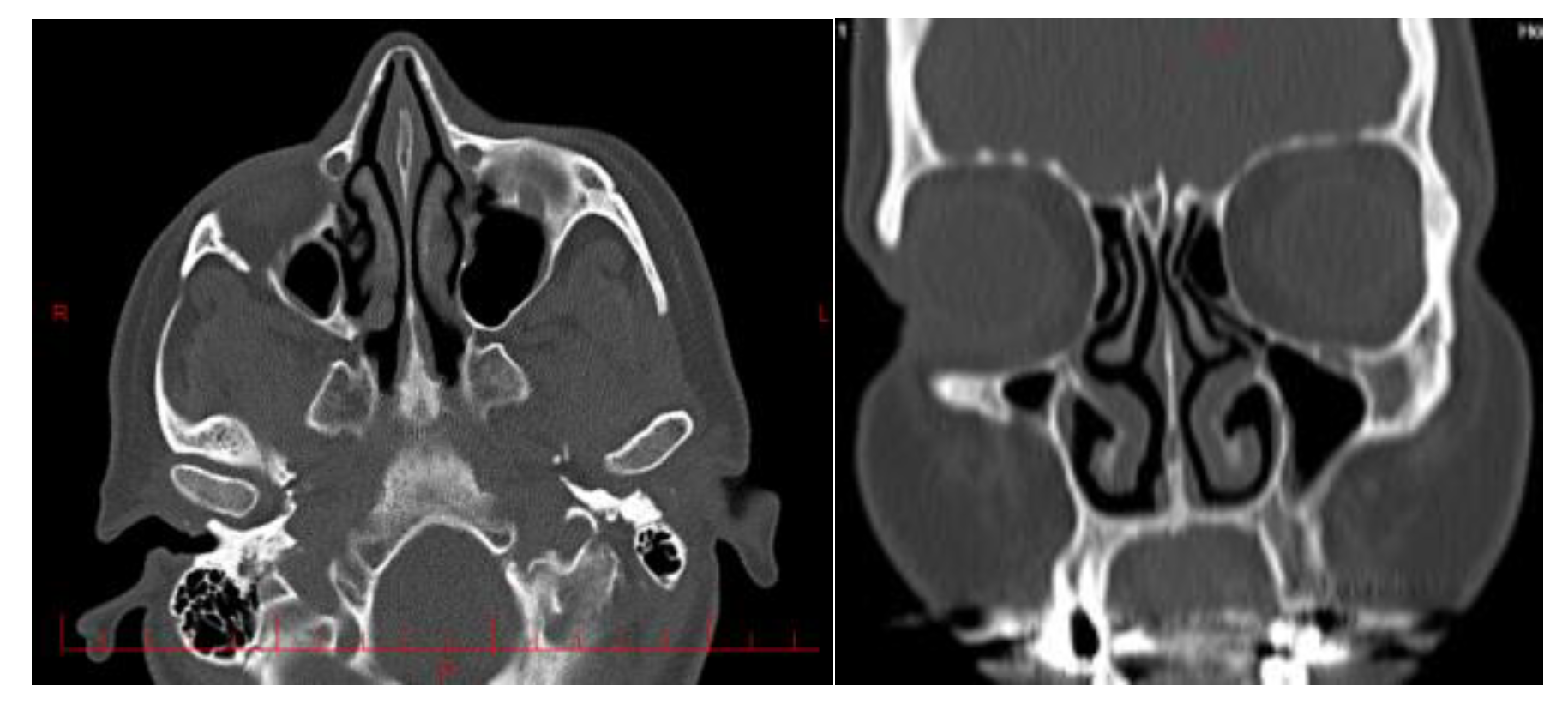
Figure 2.
Nasal cavity CT scan of patient with NSD (Axial and Coronal.
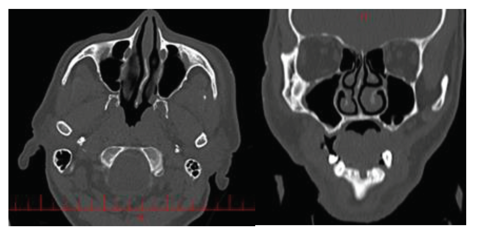
Figure 3.
Mimics output (.STL).
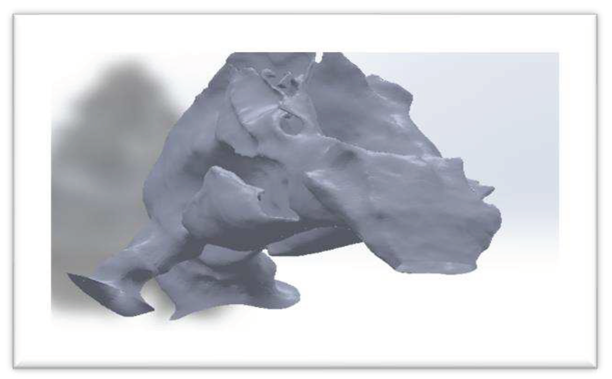
Figure 4.
CATIA ‘s output (.STEP).
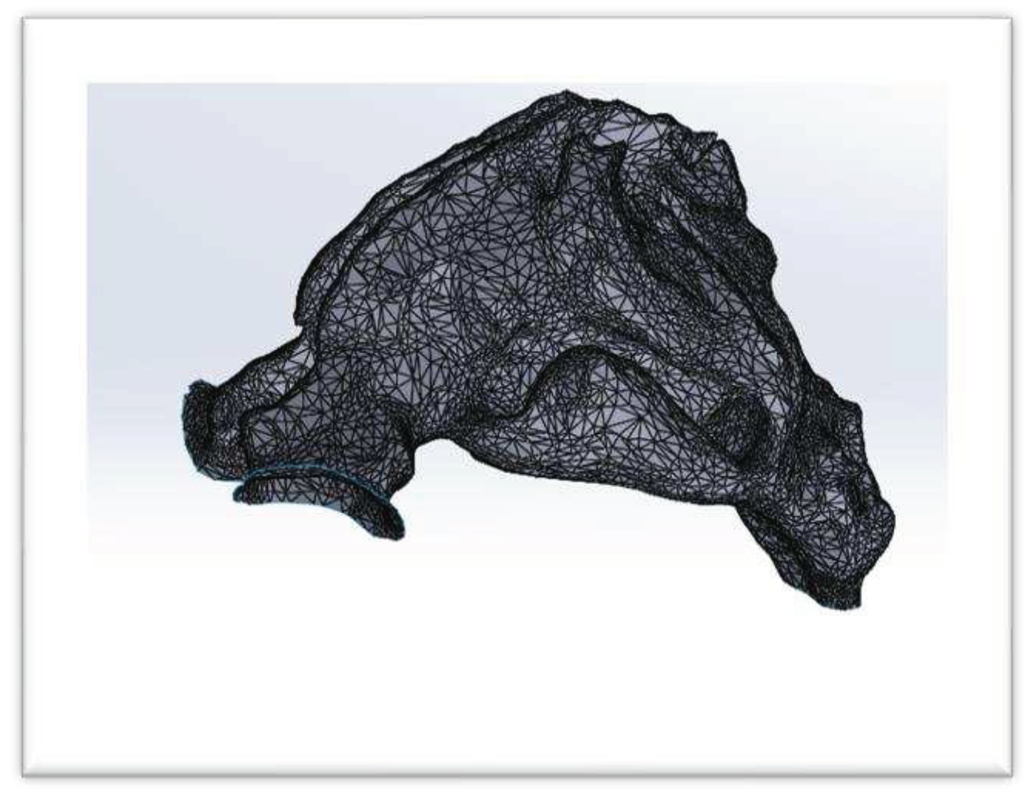
Figure 5.
Mesh generation of nasal cavity.
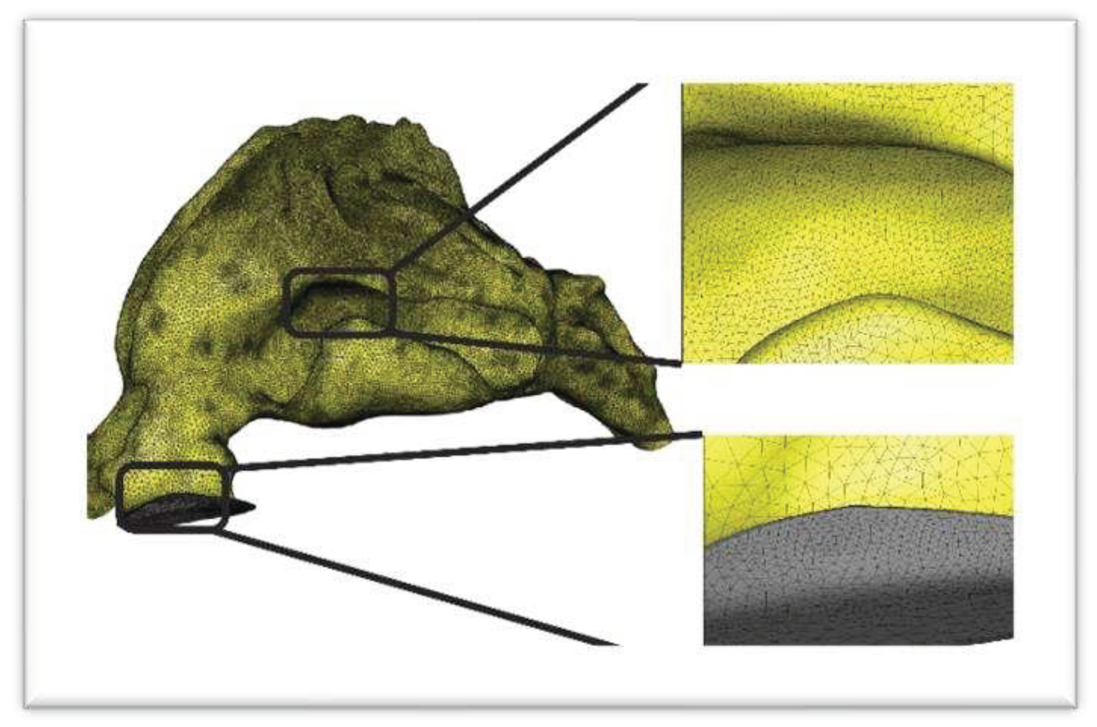
Figure 6.
solution algorithm.
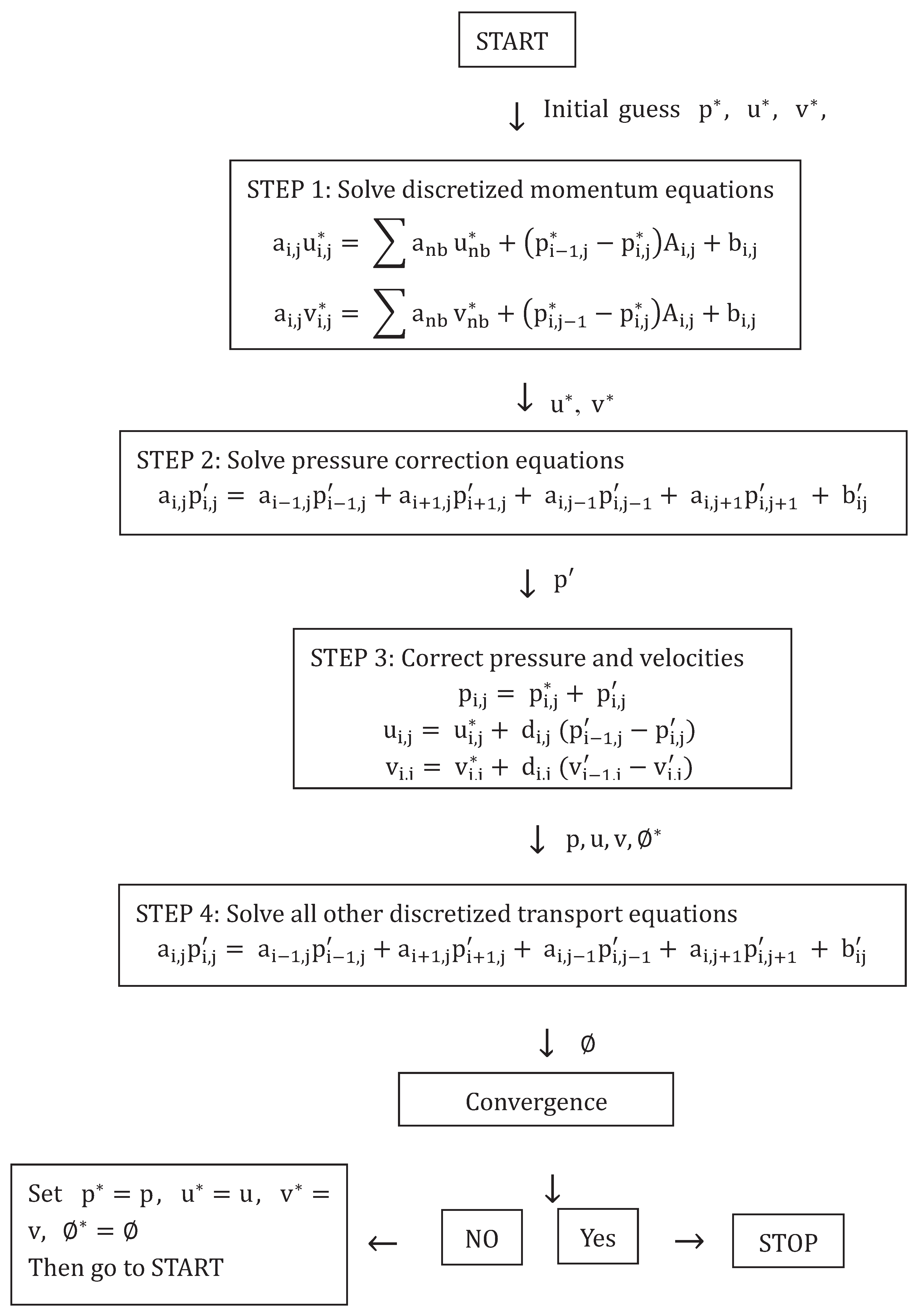
Figure 7.
Cross-sectional planes in the adult nasal cavity.
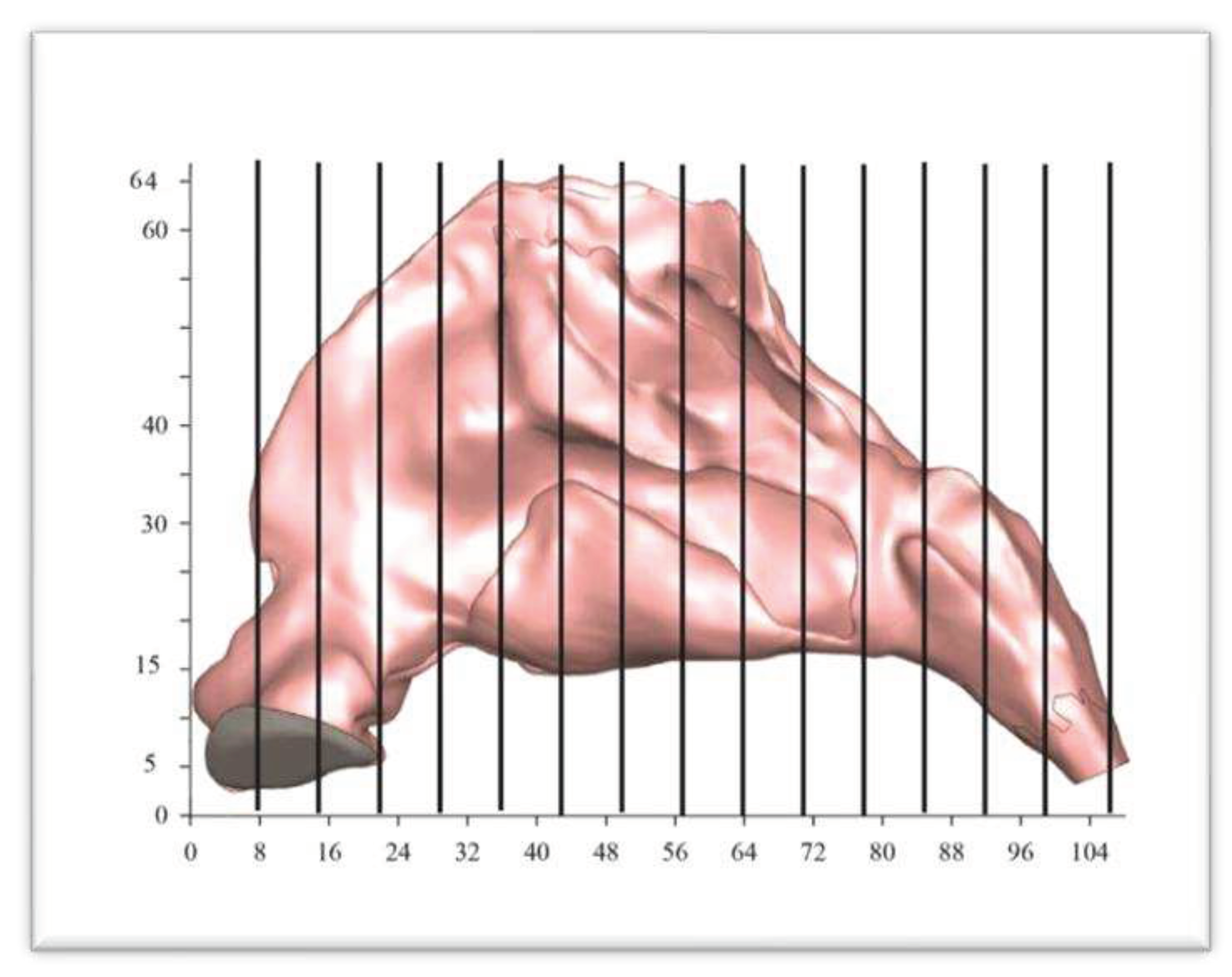
Figure 8.
Comparison of cross-sectional areas between patient with NSD and normal nasal cavity.
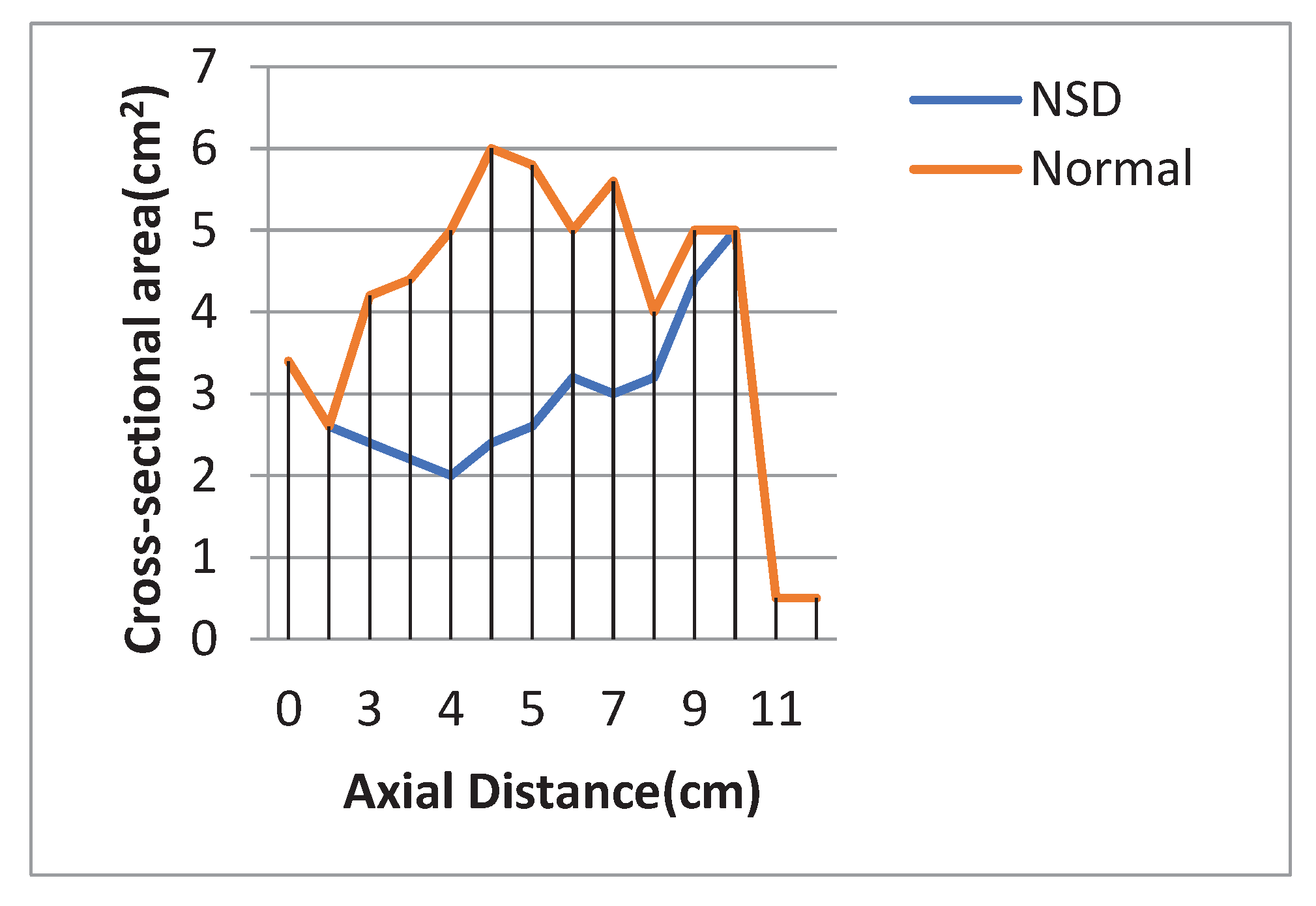
Figure 9.
Velocity contours of nasal cavity with NSD (32 mm from nasal tip).
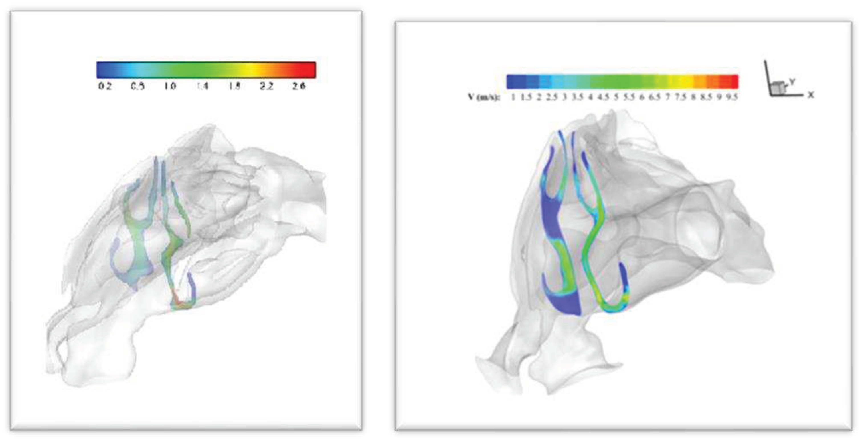
Figure 10.
Pressure distribution in NSD and normal nasal cavity.
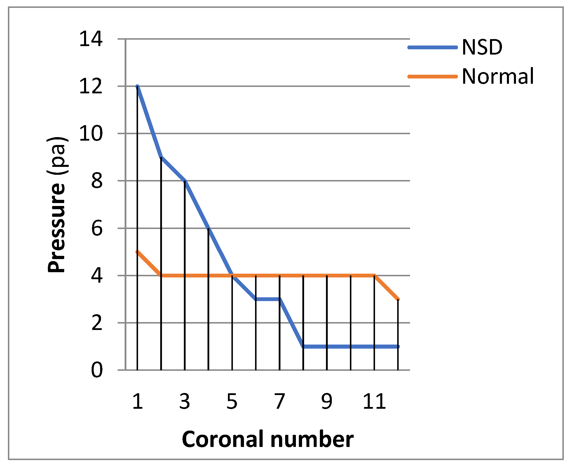
Figure 11.
WSS in NSD and normal nasal cavity.
Disclaimer/Publisher’s Note: The statements, opinions and data contained in all publications are solely those of the individual author(s) and contributor(s) and not of MDPI and/or the editor(s). MDPI and/or the editor(s) disclaim responsibility for any injury to people or property resulting from any ideas, methods, instructions or products referred to in the content. |
© 2023 by the authors. Licensee MDPI, Basel, Switzerland. This article is an open access article distributed under the terms and conditions of the Creative Commons Attribution (CC BY) license (http://creativecommons.org/licenses/by/4.0/).
Copyright: This open access article is published under a Creative Commons CC BY 4.0 license, which permit the free download, distribution, and reuse, provided that the author and preprint are cited in any reuse.


