
Submitted:
03 August 2023
Posted:
03 August 2023
You are already at the latest version
Abstract
Speaker recognition methods based on convolutional neural networks (CNN) have been widely used in the security field and smart wearable devices. However, the traditional CNN has a large number of hyperparameters that are difficult to be determined, which makes the model easy to fall into local optimum or even fail to converge during the training process. Intelligent algorithms such as particle swarm optimization and genetic algorithm are used to solve the above problems. However, these algorithms have poor performance compared with the current emerging meta-heuristic algorithms. In this study, the dung beetle optimized convolution neural network (DBO-CNN) is proposed to identify the speakers, which is helpful in finding suitable hyperparameters for training. By testing the dataset of 50 people, it was demonstrated that the accuracy of the model was significantly improved by using this approach. Compared with the traditional CNN and CNN optimized by other intelligent algorithms, the accuracy of DBO-CNN has increased by 0.6%~4.8%, and reached 98.3%.
Keywords:
speaker identification
; convolutional neural network
; dung beetle optimizer
1. Introduction
Recognition is widely used in fields such as healthcare, security, and intelligent transportation. Image recognition is a mature method that uses light waves. Similarly, sound waves are also a significant approach to identify the biometrics, e.g., speaker recognition is standing out for its convenience and reliability. A variety of voice feature extraction methods and recognition models have been investigated. The main feature extraction methods include the Linear Prediction Coding [1], the Linear Prediction Cepstral Coefficients (LPCC) [2,3] and the Mel-Frequency Cepstral Coefficients (MFCC) [4,5]. Based on the above methods, a large number of mature recognition models and applications have been proposed. Nakagawa et al., proposed a text-independent speaker recognition method based on Hidden Markov models (HMM) and Gaussian mixture model (GMM), and evaluated the robustness of the model affected by speech style [6]. Matsui et al., studied a speaker recognition method that was robust to background noise. This method combined the speaker and noise source into a noisy speaker HMM with a specific signal-to-noise ratio (SNR), and used this likelihood value to obtain recognition results [7]. Limkar et al., proposed to compare the recognition rates of multiple combination models using vector quantization and dynamic time warping, and the results showed that LPCC and MFCC had better performance [8]. Keogh et al., introduced a new technology for precise indexing, which was a model based on template matching. Using the idea of dynamic programming, they solved the problem of different pronunciation lengths, however, it could only be used in isolated word speech recognition. The effect of other application scenarios was not ideal [9]. Zheng et al., proposed the GMM Universal Background Model, which utilized the speaker's trained speech and a Bayesian adaptive form to adjust the parameters of UBM. This model reduced dependence on text and accurately identified the speaker [10]. Campbell et al., proposed the method of using GMM hypervectors in support vector machine (SVM) classifiers, and using two new SVM kernels based on distance measurement between GMM models. Experiments had shown that these SVM kernels produced excellent classification accuracy in NIST speaker recognition and evaluation tasks [11]. However, the performance of the above models is extremely vulnerable to environmental noise.
In recent years, CNN has been widely applied in the field of image recognition and object detection due to its excellent feature extraction ability, thus it can be also used in the field of speaker recognition. Achar et al., proposed a hybrid recognition method based on CNN and MFCC, which achieved a recognition accuracy of 87.5% [12]. Liu et al., proposed a new model to improve the recognition accuracy of short speech speaker recognition systems by addressing the issue of GMM being unable to accurately recognize short speech speakers, and reduce the recognition error rate from 4.9% to 2.5% [13]. Joonet et al., created the VoxCeleb2 dataset and used a deep CNN to classify it with 92.67% accuracy [14]. Jagiasi et al., described a text-independent CNN model for speaker recognition, and achieved recognition rates of 75% to 85% [15]. Wang et al., proposed a voiceprint recognition model based on Mel time-spectrum convolutional neural network for identifying faults in transformers during operation. This method constructed a CNN model by feature extraction preprocessing and Mel filter. This model could recognize the voiceprint of transformers by four different operating faults [16]. However, the hyperparameter settings of CNNs had a large impact on model performance, and the work was usually based on trial-and-error or experience. Population-based intelligent algorithms such as genetic algorithm (GA) and particle swarm optimization (PSO) were used to optimize the hyperparameters of CNN [17,18,19,20]. Yoo et al., proposed a method of optimizing CNN with GA and tested image recognition on the MNIST dataset, and achieved an accuracy rate of 99.4% [17]. Ishaq et al., used GA to adjust the hyperparameters of CNN, and achieved an accuracy rate of 95.5% in the emotion recognition test, which had a great advantage over other methods [18]. Chen et al., proposed a PSO-optimized adaptive CNN(PSO-CNN) to analyze the spectrogram during the working process of the bearing to determine whether the bearing was damaged. This method had a recognition accuracy rate of 99.9% for the four damage situations [19]. Bhuvansehwari et al., used the dragonfly optimizer based on information gain and the CNN classifier optimized by particle PSO based on depth clustering to identify network attack aircraft types. The optimization algorithm could reduce clustering losses and network losses [20]. The above studies showed that these optimization methods were effective for improving the performance of CNN. After decades of scientific and technological development, the above-mentioned intelligent algorithms have shown limited effects in current complex and huge engineering problems.
Researchers have proposed many heuristic search algorithms Inspired by nature that imitate various biological habits. These algorithm models have two core survival strategies of biological populations, role division and behavioral differentiation. Role division refers to the use of fitness to divide the population into different groups, while behavioral difference means that individuals in different groups have different action strategies. In population, the role played by each individual is not static. During the foraging process, the fitness of individuals will change, which will change their role. But no matter how the population is divided, the ultimate goal of all individuals is the same, that is to find the most suitable habitat for the survival and reproduction of the population. In particular, the action strategies of individuals in bionic algorithms are more reasonable and effective, because the objects they imitate are multiplying and thriving in real life. In recent years, the Whale Algorithm [21], Grey Wolf Optimization [22], Sparrow Search Algorithm (SSA) [13] and Jumping Spider Optimization Algorithm [24] were heuristic algorithms proposed based on the above ideas which were with efficient search capabilities. They have been applied in many fields.
In this study, the DBO is used to optimize the hyperparameters of the CNN to identify speakers. DBO is the latest heuristic algorithm proposed by Xue et al., with excellent exploration and high local optimal avoidance ability [25]. This algorithm simulates the stratum distribution and foraging habits in the dung beetle group, and uses different foraging strategies to find the optimal solution within a certain range, which is the first time this algorithm has been used to optimize CNNs. In addition, a comparison between the DBO with the other algorithms is proposed, and the experimental results demonstrate the superiority of DBO in optimizing CNN hyperparameters. This paper is structured as follows: Sec. II shows the processing flow of audio data. Sec. III introduces CNN model architecture and DBO calculation process. Sec. IV shows the result and discussion about optimized CNN. Sec. V presents conclusions and future work.
2. Preliminary Work
2.1. Speaker Recognition in CNN
The process of using CNN for speaker recognition includes two parts, the generation of spectrogram and the calculation of CNN, as shown in Figure 1. Firstly, convert the audio signal into spectrum diagram data, and then import the obtained images into CNN for feature extraction and classification. Finally, accurately identify the speaker.
2.2. Generation of Spectrogram
Since two-dimensional data is used in CNN, it is necessary to expand the dimension of audio data. The spectrogram is an image that displays the audio frequency spectrum, which denotes the variation of the frequency and amplitude of a speech signal over time. In the spectrogram, the energy of sound is displayed in the form of texture, which is called voiceprint. Voiceprint contains a lot of speaker characteristics, and everyone's voiceprint is different. The essence of speaker recognition is to extract and classify voiceprints.
As shown in Figure 2, the production process of the spectrogram is divided into five steps: i) pre-emphasis is used to enhance the high-frequency content of the signal to compensate for the loss during the acquisition process; ii) due to the short-term stability of the voice signal, the audio signal is decomposed into some small fragments, and then the Hanning window is added to these fragments; iii) the amplitude-frequency characteristics of the above speech segment sequence are obtained after the fast Fourier transform (FFT) processing, and then the modulus is taken to obtain the transformed linear spectrum; iv) a linear spectrum is converted into a spectrogram by the logarithmic transformation; v) color mapping is used to add details and features to the image and resize the image for CNN recognition.
2.3. CNN Architecture
As shown in Figure 3, CNN can be functionally divided into two parts, feature extraction and classification. The feature extraction is composed of two-dimensional convolutional layers and pooling layers stacked in a certain order. The number of filters in each convolutional layer corresponds to the number of features currently expected to be extracted from the image, and the pooling layer abstracts it to a higher level while reducing the size of the image. The classification is the combination of the full connection layer and the activation function, which maps the extracted features to the sample space, and nonlinear calculations are utilized to improve the expressiveness of the network by the activation function.
When building a CNN, there are numerous hyperparameters that need to be determined. The hyperparameter types that this study focuses on are as follows:
- The number of filters per convolution layer: this parameter determines the abstraction ability of the network and the number of features to be extracted eventually;
- The number of neurons in the fully connected layer: too few neurons may result in failure to train a model that meets the requirements, while numerous neurons may lead to overfitting;
- Learning rate: if the learning rate is too low, it is easy for the model to fall into a local optimum, and if it is too high, it is easy to miss the global optimum and fail to complete the training.
It is not simple to build and train CNN with good performance, which requires a lot of time and cost. Therefore, there is an urgent need for a method that can automatically build CNN in various tasks, which can help people determine various kinds of super parameters.
3. Proposed Approaches
3.1. Resnet
CNNs significantly outperform other traditional classifier models in the field of image recognition. However, as the depth of the model increases, problems such as gradient disappearance and gradient explosion will degrade the model and make the performance of the model worse. The fundamental reason is that the parameters of the lower convolution kernel are difficult to be effectively adjusted in the later stage of training. In order to solve the above problems, some scholars proposed a deep residual network (ResNet). ResNet directly transmits low-level features to higher levels by introducing residual blocks, which makes it more capable of feature extraction and representation. This connection mode will not be affected by the depth of the network.
As shown in Figure 4, Resnet contains many residual blocks. There are two parts of each block: short cut and convolution calculation. Short cut maps the image of the previous layer directly to the next layer. The convolution calculation includes several convolution kernels, batch normalization (BN) and activation functions. BN aims to normalize the same batch of data into standard normal distribution, which can make the model converge quickly.
The calculation process of the whole residual can be described as:
where F represents the convolution calculation of the block, represents weight and offset parameters, H represents the short cut, and , are the input and output, respectively.
A large number of different models of ResNet are developed by stacking different number of residual blocks, ResNet18/43 and ResNet50/101/152. The optimization method proposed in this study is applied to ResNet18.
3.2. DBO
DBO that was inspired by the biological behavior process of dung beetles, is a swarm intelligent optimization algorithm with strong optimization ability and fast convergence speed. In a beetle population, differences in food abundance at foraging locations among individuals lead to differences in fitness. By using the fitness ranking as a division criterion, these individuals were divided into four different roles in descending order of fitness: ball-rolling beetles, brood balls, small beetles, and thief beetles. Rolling ball beetles are individuals with high fitness. Their goal is to move the food ball to a place suitable for breeding. When the female beetle finds the food ball of the rolling ball beetle, it will move it for a short distance and lay eggs on it, which is called the brood ball. After hatching, the baby beetle will look for food around the brood ball. Thief beetles will snatch the food balls of other beetles. Each role corresponds to a specific adjustment strategy of position. After each foraging, the fitness ranking of each individual redefines their roles in the next foraging. Based on fitness ranking, the mechanism of role division helps individuals optimize strategies of foraging behavior according to their fitness level, so as to find a suitable location for the survival and reproduction of the population. The location update formula of ball-rolling beetles is given as:
where represents the position of the dimension of the beetle in the iteration, is a natural coefficient which is assigned -1 or 1, denotes a constant value which indicates the deflection coefficient, b is a constant from 0 to 1, is the deflection angle, R is a random number belonging to (0,1), when , beetle has encountered obstacles and needs to adjust its direction, indicates the changes of light intensity , represents the current global worst position.
The position update formula of brood balls can be expressed as:
where denotes the current local best position, Lb and Ub represent the upper and lower bounds of the search area respectively, and represent the upper and lower bounds of the spawning area, respectively. and represent two independent random D-dimensional vectors belongs to (0,1), D is the dimension of the optimization problem.
The position update formula of small beetles can be expressed as:
where denotes the global best position, and represent the upper and lower bounds of the optimal foraging area respectively. belongs to (0,1), which follows normally distributed, represent a random D-dimensional vector.
The location update formula of thief beetles is given as:
where S represent a constant value, g is a random D-dimensional vector that follows normally distributed.
3.3. Optimization Process
ResNet18 has five residual blocks. We need to determine the number of output channels or convolution kernel for the five residual blocks. In order to improve the expression ability of the network, an additional hidden layer is added to the full connection layer, thus the number of neurons with two hidden layers needs to be determined. Finally, we need to determine the learning rate in the training process. All hyperparameters and their ranges that need to be optimized for this model are shown in Table 1. The dimension that beetles need to search is 8. The calculation method of beetle fitness is described as, decoding the position coordinates into hyperparameters, and then using these hyperparameters to establish ResNet18. After a training, the test set is led into testing, and the obtained accuracy is the fitness of the beetle.
The process of speaker recognition using DBO-CNN is shown in Figure 5, which can be divided into five steps:
- Step I, divide the data set into a training set and a test set in a ratio of about 8:2;
- Step II, initialize the population and divide it into different beetle roles according to the fitness ranking. Among them, ball-rolling beetles accounts for 6/30, brood balls accounts for 6/30, small beetles accounts for 7/30 and thief beetles accounts for 11/30;
- Step III, the beetles search for the optimal hyperparameter group according to their own strategies of position adjustment;
- Step IV, build a convolutional neural network for speaker recognition by using the optimal hyperparameters;
- Step V, evaluate the model on the test set after training.
4. Experiments and Results
4.1. Dataset
The data set used in this study is the Chinese Mandarin open source voice database from Hill Shell. The database contains voice data covering voice control, unmanned driving, industrial production and other fields. In order to increase the richness of the database, the database is built by recruiting 400 people from different accent regions in China to participate in the recording.
The voice data of 50 people with 300 to 400 voice messages for each person are randomly selected. These voices are cut into 2.5s long segments, and each segment contains 40000 data points. When using FFT to make spectrogram, set the length of Hanning window to 256, and the moving width of each frame to 128, which is half of the window length. Finally, the obtained spectrograms are normalized to 128 × 128. The data sets contain 17265 images. The number of images is 14605 for training sets and 3200 for test sets.
4.2. Hyperparameters Optimization
DBO provides an efficient guide for determining the hyperparameters of CNN, however it also has some population-related constants to be set. In this study, the constants are used as the same with the author of DBO: k = 0.1, b = 0.3, S = 0.5. In order to evaluate the performance of DBO-CNN, we compared it with PSO-CNN, Sparrow Algorithm Optimized CNN (SSA-CNN), and CNN built by experience. In the three optimization processes, the population and search times are set to 50 and 30. After iteration, the hyperparameters found by the three algorithms are shown in Table 2, and the hyperparameters chosen empirically are also listed.
4.3. Model Training
The CNNs using the above four sets of hyperparameters are constructed, and the produced spectrograms are imported into them for training. The loss function is SoftMaxCrossEntropy. The number of iterations is set to 50.
As shown in Figure 6, the loss of traditional CNN does not decrease below 0.01 after 50 iterations, which is the worst in the model. DBO-CNN performs the best by reducing losses to below 0.01 after only 5 iterations, PSO-CNN spends 25 times, and SSA-CNN spends 21 times, which indicates that DBO significantly improves the training speed of the model. The evaluation results of the four models on the test set are shown in Figure 7. After the optimization of the intelligent algorithm, the accuracy of the model has been significantly improved. Among them, DBO-CNN has the greatest improvement with the accuracy rate of 98.34%, followed by SSA-CNN with the accuracy rate of 97.71%, and finally PSO-CNN with the accuracy rate of 95.62%. It is demonstrated that DBO is indeed superior to traditional intelligent algorithms such as PSO.
4.4. Noise Resistance Test
Due to environmental noise interference or performance limitations of recording equipment, the effects of the audio are always unsatisfactory. In order to test the anti-interference ability of the model in this environment, some white noise is added to the previous test set data. We tested the performance of the model by different signal-to-noise ratios. As shown in Figure 8, as the proportion of noise increases, the recognition accuracy of all models decreases. The anti-noise ability of the two newer meta heuristic algorithms is basically the same, and the accuracy is still around 80% in a signal-to-noise ratio environment of 30 dB. Even in a harsh environment of 20 dB, the accuracy of both algorithms is above 50%, which is acceptable. However, the accuracy of particle algorithms and traditional CNN in noisy environments has significantly decreased, and their anti-noise performance is significantly weaker than the new meta heuristic algorithm.
5. Conclusions and Future Work
A DBO-CNN algorithm is proposed for speaker recognition in this study, and compared with the other three algorithms on a dataset of 50 people. After optimization, the performance of all models has improved. Compared to other algorithms, DBO-CNN has better optimization ability. It not only has the fastest convergence speed, but also has the highest accuracy, reaching 98.34%. In terms of anti-interference, DBO-CNN and SSA-CNN have similar performance, and their recognition rates are both above 50% in harsh environments of 20 dB. Based on the results, it demonstrates that speaker recognition has been greatly improved by the DBO-CNN compared with other optimization algorithms, and also illustrates that DBO has the enormous potential in optimizing CNN.
The future work is to expand the scale of the dataset and deploy the model on embedded devices, and a synthetic approach to measure the performance of the indexes will be used to speaker recognition [26]. As well as, swarm intelligence is a promising and challenging science subbranch. In 2021, the Nobel Physics Award is partially grant to the work about the swarm behavior and intelligence. Meanwhile, new developments from multiple fields are deepening broadening the cognition on swarm intelligence. For swarm intelligent method based on bionic computing, some recent biological achievements such as adaptive mutability [27], epigenetics [28] are sure to improve the performance of speaker recognition. These swarm optimization algorithms will be attempted for further research.
Author Contributions
Conceptualization, X. G. and Z. F.; methodology, X. Q.; validation, X. Q.; investigation, Y.Z. and Q.Z.; data curation, X. Q.; writing—original draft preparation, X. G.; writing—review and editing, P. W. and Z. F.; supervision, P. W. and Z. F. All authors have read and agreed to the published version of the manuscript.
Funding
This research was funded by The Open Project of Key Lab of Digital Signal and Image Processing of Guangdong Province.
Institutional Review Board Statement
Not applicable.
Informed Consent Statement
Not applicable.
Data Availability Statement
Not applicable.
Conflicts of Interest
The authors declare no conflict of interest.
References
- Gupta, H.; Gupta, D. LPC and LPCC method of feature extraction in Speech Recognition System. In Proceedings of the 2016 6th International Conference - Cloud System and Big Data Engineering (Confluence), Noida, India, 14-15 January 2016; pp. 498-502. [CrossRef].
- Chia Ai, O.; Hariharan, M.; Yaacob, S.;Sin Chee, L. Classification of speech dysfluencies with MFCC and LPCC features. Expert Systems with Applications 2012, 39, 2157-65. [CrossRef]. [CrossRef]
- Tripathi, A.; Singh, U.; Bansal, G.; Gupta, R.; Singh, A.K. A Review on Emotion Detection and Classification using Speech. In Proceedings of the International Conference on Innovative Computing & Communications (ICICC) 2020, New Delhi, India, 21-23 February 2020. [CrossRef].
- Tiwari, V. MFCC and its applications in speaker recognition. International journal on emerging technologies 2010, 1, 19-22. [CrossRef].
- Bhadragiri, J. M.; Ramesh, B. N. Speech recognition using MFCC and DTW. In Proceedings of the 2014 International Conference on Advances in Electrical Engineering (ICAEE), Vellore, India, 9-11 January 2014; pp. 1-4. [CrossRef].
- Nakagawa, S.; Zhang, W.; Takahashi,M. Text-independent speaker recognition by combining speaker-specific GMM with speaker adapted syllable-based HMM. In Proceedings of the 2004 IEEE International Conference on Acoustics, Speech, and Signal Processing, Montreal, QC, Canada, 30 August 2004; pp. I-81. [CrossRef].
- Matsui, T.; Kanno,T.; Furui,S. Speaker recognition using HMM composition in noisy environments. Computer Speech & Language 1996, 10, 107-116. [CrossRef]. [CrossRef]
- Limkar, M.; Rao,B.R.; Sagvekar, V. Speaker Recognition using VQ and DTW. International Journal of Computer Applications 2012, 3, 975-8887. [CrossRef].
- Keogh, E.; Ratanamahatana, C.A. Exact indexing of dynamic time warping. Knowledge and Information Systems 2005, 7, 358-386. [CrossRef]. [CrossRef]
- Rong, Z.; Shuwu, Z.; Bo, X. Text-independent speaker identification using GMM-UBM and frame level likelihood normalization. In Proceedings of the 2004 International Symposium on Chinese Spoken Language Processing, Hong Kong, China, 15-18 December 2004; pp. 289-292. [CrossRef].
- Liu, Z.; Wu, Z.; Li, T.; Li, J.; Shen, C. GMM and CNN Hybrid Method for Short Utterance Speaker Recognition. IEEE Transactions on Industrial Informatics 2018, 14, 3244-3252. [CrossRef]. [CrossRef]
- Campbell, W.M.; Sturim, D.E.; Reynolds, D.A. Support vector machines using GMM supervectors for speaker verification. IEEE Signal Processing Letters 2006, 13. [CrossRef]. [CrossRef]
- Wang, S.; Zhao, B.; Du, J. Research on transformer fault voiceprint recognition based on Mel time-frequency spectrum-convolutional neural network. Journal of Physics: Conference Series 2022, 2378, 12-89. [CrossRef]. [CrossRef]
- Ashar, A.; Bhatti, M.S.; Mushtaq,U. Speaker Identification Using a Hybrid CNN-MFCC Approach. In Proceedings of the 2020 International Conference on Emerging Trends in Smart Technologies (ICETST), Karachi, Pakistan, 26-27 March 2020; pp. 1-4. [CrossRef].
- Chung, J.S.; Nagrani, A.; Zisserman, A. Voxceleb2: Deep speaker recognition. arXiv 2018, arXiv:1806.05622 [CrossRef].
- Jagiasi, R.; Ghosalkar, S.; Kulal, P.; Bharambe, A. CNN based speaker recognition in language and text-independent small scale system. In Proceedings of the 2019 Third International conference on I-SMAC (IoT in Social, Mobile, Analytics and Cloud) (I-SMAC), Palladam, India, 12-14 December 2019; pp. 176-179. [CrossRef].
- Yoo, J.H.; Yoon,H.I.; Kim, H.G.; Yoon, H.S.; Han, S.S. Optimization of Hyper-parameter for CNN Model using Genetic Algorithm. In Proceedings of the 2019 1st International Conference on Electrical, Control and Instrumentation Engineering (ICECIE), Kuala Lumpur, Malaysia, 25-25 November 2019; pp. 1-6. [CrossRef].
- Ishaq, A.; Asghar, S.; Gillani, S.A. Aspect-Based Sentiment Analysis Using a Hybridized Approach Based on CNN and GA. IEEE Access 2020; 8, 135499-135512. [CrossRef]. [CrossRef]
- Chen, J.; Jiang, J.; Guo, X.; Tan, L. A self-Adaptive CNN with PSO for bearing fault diagnosis. Systems Science & Control Engineering 2020, 9, 11-22. [CrossRef]. [CrossRef]
- Bhuvaneshwari, K.S.; Venkatachalam, K.; Hubálovský, S.; Trojovský P.; Prabu, P. Improved Dragonfly Optimizer for Intrusion Detection Using Deep Clustering CNN-PSO Classifier. Computers, Materials & Continua 2022, 70. [CrossRef].
- Mirjalili, S.; Lewis, A. The whale optimization algorithm. Advances in engineering software 2016, 95, 51-67. [CrossRef].
- Mirjalili, S.; Mirjalili, S.M.; Lewis, A. Grey wolf optimizer. Advances in engineering software 2014, 69, 46-61. [CrossRef].
- Xue, J.; Shen, B. A novel swarm intelligence optimization approach: sparrow search algorithm. Systems science & control engineering 2020, 8, 22-34. [CrossRef]. [CrossRef]
- Peraza-Vázquez, H.; Peña-Delgado, A.; Ranjan, P.; Barde, C.; Choubey, A.; Morales-Cepeda, A.B. A bio-inspired method for mathematical optimization inspired by arachnida salticidade. Mathematics 2021, 10, 102. [CrossRef]. [CrossRef]
- Xue, J.; Shen, B. Dung beetle optimizer: a new meta-heuristic algorithm for global optimization. The Journal of Supercomputing 2023, 79, 7305-7336. [CrossRef]. [CrossRef]
- Wang, P.; Zhang, J.; Xu, L.; Wang, H.; Feng, S.; Zhu, H. How to measure adaptation complexity in evolvable systems–A new synthetic approach of constructing fitness functions. Expert Systems with Applications 2011, 38, 10414-10419. [CrossRef]. [CrossRef]
- Reilly, N.; Arena1, S.; Lamba, S.; Bartolini, A.; Amodio, V.; Magrì, A.; Novara, L.; Sarotto, I.; Nagel, Z.D.; Piett, C.G.; Amatu, A.; Sartore-Bianchi, A.; Siena, S.; Bertotti, A.; Trusolino, L.; Corigliano, M.; Gherardi, M.; Lagomarsino, M.C.; Nicolantonio, F.D.; Bardelli, A. Adaptive mutability of colorectal cancers in response to targeted therapies. Science 2019, 366, 1473-1480. [CrossRef]. [CrossRef]
- Pan, Z.; Yao, Y.; Yin, H.; Cai, Z.; Wang, Y.; Bai, L.; Kern, C.; Halstead, M.; Chanthavixay, G.; Trakooljul, N.; Wimmers, K. Sahana, G.; Su, G.; Lund, M.S.; Fredholm, M.; Karlskov-Mortensen, P.; Ernst, C.W.; Ross, P.; Tuggle, C.K..; Fang, L.; Zhou, H. Pig genome functional annotation enhances the biological interpretation of complex traits and human disease. Nat Commun 2021, 12, 5848. [CrossRef].
Figure 1.
The process of recognizing the speaker.
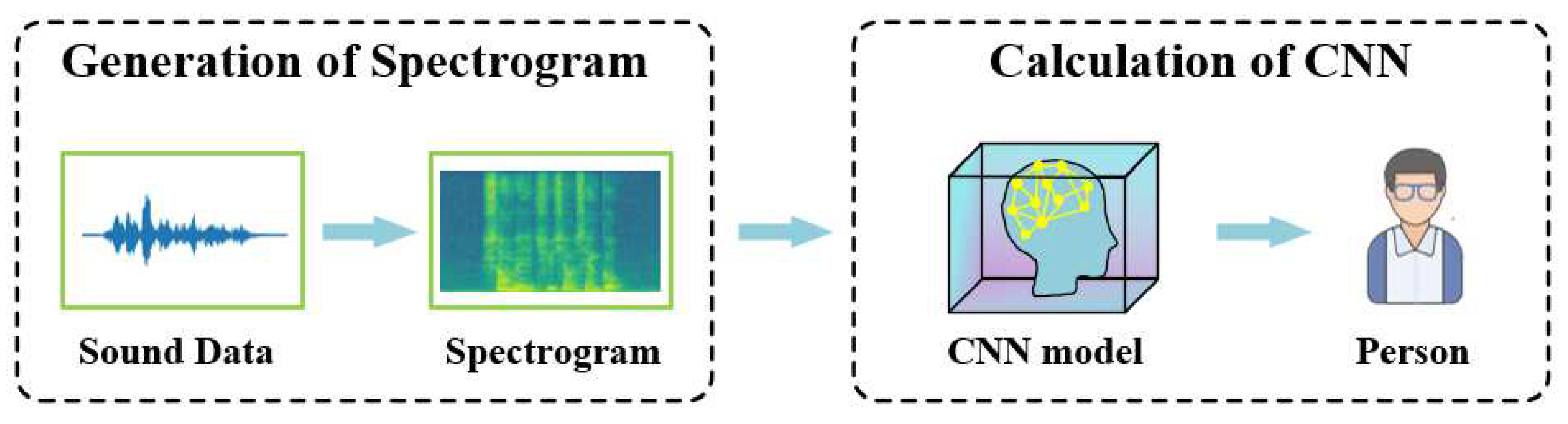
Figure 2.
Generation process of spectrogram.

Figure 3.
The CNN architecture.
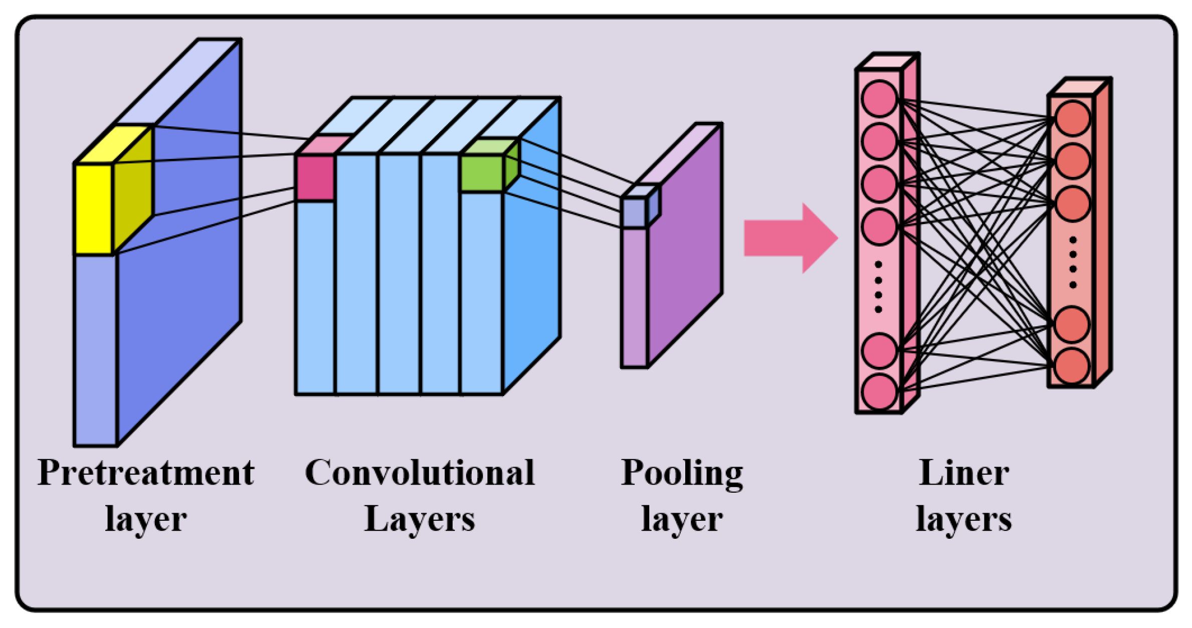
Figure 4.
The composition of Resnet and the structure of the residual block.

Figure 5.
The process for recognizing speakers by using the optimized DBO.

Figure 6.
Comparison on loss of Four Different CNN Models during Training. (a) The Loss Curve of Traditional CNN, (b) the Loss Curve of PSO-CNN, (c) the Loss Curve of SSA-CNN, and (d) the Loss Curve of DBO-CNN.
Figure 6.
Comparison on loss of Four Different CNN Models during Training. (a) The Loss Curve of Traditional CNN, (b) the Loss Curve of PSO-CNN, (c) the Loss Curve of SSA-CNN, and (d) the Loss Curve of DBO-CNN.

Figure 7.
Accuracy of the models CNN, PSO-CNN, SSA-CNN, and DBO-CNN.

Figure 8.
Recognition accuracy of four models by different signal-to-noise ratios.


Table 1.
Hyperparameters searched by different models.
| Layer | Range |
|---|---|
| residual block 1 | 16~32 |
| residual block 2 | 32~64 |
| residual block 3 | 64~128 |
| residual block 4 | 128~256 |
| residual block 5 | 256~512 |
| residual block 1 | 512~1024 |
| linear layer 1 | 256~512 |
| linear layer 2 | 64~128 |
| learning rate | 1e2~1e-3 |
Table 2.
Hyperparameters searched by different models.
| Layer | CNN | PSO-CNN | SSA-CNN | DBO-CNN |
|---|---|---|---|---|
| residual block 1 | 32 | 24 | 27 | 21 |
| residual block 2 | 64 | 32 | 54 | 63 |
| residual block 3 | 128 | 117 | 107 | 71 |
| residual block 4 | 256 | 230 | 143 | 256 |
| residual block 5 | 512 | 386 | 424 | 272 |
| linear layer 1 | 1024 | 424 | 904 | 653 |
| linear layer 2 | 512 | 272 | 394 | 259 |
| learning rate | 1e-2 | 1e-3 | 1e-3 | 1e-3 |
Disclaimer/Publisher’s Note: The statements, opinions and data contained in all publications are solely those of the individual author(s) and contributor(s) and not of MDPI and/or the editor(s). MDPI and/or the editor(s) disclaim responsibility for any injury to people or property resulting from any ideas, methods, instructions or products referred to in the content. |
© 2023 by the authors. Licensee MDPI, Basel, Switzerland. This article is an open access article distributed under the terms and conditions of the Creative Commons Attribution (CC BY) license (http://creativecommons.org/licenses/by/4.0/).
Copyright: This open access article is published under a Creative Commons CC BY 4.0 license, which permit the free download, distribution, and reuse, provided that the author and preprint are cited in any reuse.


