Submitted:
02 August 2023
Posted:
03 August 2023
You are already at the latest version
Abstract
Defect recognition in ballastless track structures, based on distributed acoustic sensors (DASs), was researched in order to improve detection efficiency and ensure the safe operation of trains on high-speed railways. A line in southern China was selected, and equipment was installed and debugged to collect the signals of trains and events along it. Track vibration signals were extracted by identifying a train track, denoising, framing and labeling to build a defect dataset. Time–frequency-domain statistical features, wavelet packet energy spectra and the MFCCs of vibration signals were extracted to form a multi-dimensional vector. An XGBoost model was trained and its accuracy reached 89.34%. A time-domain residual network (ResNet) that would expand the receptive field and test the accuracies obtained from convolution kernels of different sizes was proposed, and its accuracy reached 94.82%. In conclusion, both methods showed good performance with the built dataset. Additionally, the ResNet delivered more effective detection of DAS signals compared to conventional feature engineering methods.
Keywords:
DAS
; ballastless track
; defects recognition
; XGBoost
; ResNet
1. Introduction
In recent years, China's high-speed railway has developed rapidly. By the end of 2022, its operating mileage reached 42000 kilometers. People have put forward greater requirements for the running speed, safety and riding comfort of trains, which has made slab ballastless tracks widely used in high-speed railway construction. Compared with ballasted tracks, ballastless tracks are smooth, stable and durable. However, because this type of track contains no ballast buffer, trains will have stronger impacts on these tracks when they pass at high speed. At the same time, these tracks’ rigid concrete structures not only bring to light the dangers of new, hidden defects but also create certain difficulties for later maintenance.
With increased service life and under the impacts of high-speed trains and various environmental loads, ballastless tracks will suffer from cracks, damages and other defects [1,2,3], as shown in Figure 1. If these defects cannot be dealt with in time, the tracks will further deteriorate under the impacts and vibration of trains, which will not only seriously affect the strength of the track structure and reduce the life of the track slab but also increase the maintenance cost later. Therefore, it is of great significance to detect defects in ballastless tracks, find hidden dangers and prevent them in time.
At present, defect detection for ballastless tracks is mainly carried out through a combination of manual inspection and comprehensive detection train. However, with sharp increases in operating mileages and the fact that manual inspections can only be performed during "skylight", heavy workloads and low efficiency are problems.
In terms of technical defense, ground-penetrating radar [4,5] is used to detect the structural layer defects of ballastless tracks. However, it is difficult to identify the actual radar profiles recorded with it because of the reflection and scattering of targets, the non-uniformity of the medium distribution and the complexity and diversity of geological structures during the underground propagation of electromagnetic waves. In addition, the uncertain factors in the manual interpretation of images will ultimately affect the judgment of the result.
Distributed acoustic sensors (DAS) based on the phase-sensitive optical-time-domain reflectometer (Φ-OTDR) [6] are a new type of sensing technology that uses the interference effect of optical-fiber-back Rayleigh scattering to realize the continuous distributed detection of acoustic signals. DASs not only have the advantages of anti-EMI, non-corrosiveness and no required power supply but also can detect and locate weak vibration signals along optical fibers. They have been widely applied in fields [7,8,9,10,11,12] such as oil pipeline security monitoring, perimeter security and rail transit. Collecting the vibration signals of trains and events along a line by using DAS technology combined with signal processing, deep learning and other ways to identify track defects has provided a reliable helper method that has important application value for the safe and high-quality development of high-speed railways.
For this paper, we have studied identification technology for ballastless track defects, collected and processed vibration signals and built a defect dataset. According to the design principles of ballastless tracks and the characteristics of the sample data, two pattern recognition methods, based on feature engineering and deep learning, were proposed to verify the feasibility of DAS technology for defect detection in ballastless tracks.
2. Data Acquisition and Processing
2.1. Experimental Setup
In the field, a high-speed railway line (length: 26214.4m) in southern China was selected for track vibration signal acquisition. The sensing fiber-optic adopted the existing communication fiber-optical cable in the groove outside the line, as shown in Figure 2.
The DAS equipment (a coherent detection-based Φ-OTDR system) was placed in the communication room of the nearby station. The key parameters of the equipment are shown in Table 1. Figure 3 shows the vibration states at certain moments on the line; the X-axis represents the spatial sampling points on the optical fiber, corresponding to real geographical locations, and the Y-axis represents the phases or amplitudes of the sampling points.
2.2. Moving Average and Moving Differential Method
Optical loss is inevitable. When light with a wavelength of 1330 nm or 1550 nm propagates in a G652 single-mode fiber, the average losses per kilometer are 0.35dB and 0.25dB, respectively. The splice loss caused by fiber core fusion is about 0.05dB/piece. These losses directly lead to Rayleigh scattered light being strong at the near and weak at the far end. At the same time, due to this light’s high sensitivity, it is very easily disturbed by noise in the surrounding environment, such as construction noise along the line or traffic noise in parallel sections of highways and railways. Collected signals are mixed with many unknown noises, which may affect the positioning accuracy of DAS equipment.
To reduce noise and increase frequency responses, the moving average and moving differential method [13,14] was used in our detection system. This method consists of acquiring a certain number N of Rayleigh backscattering traces and choosing a number of the acquired traces M to be averaged. Thus, N – M + 1 subsets of averaged traces can be obtained with the noise power in a measurement reduced by a factor of 1/M. We performed filtering of the vibration signals generated by the train running at different times and obtained different results, as shown in Figure 4.
3. Vibration Signal Extraction
Defects in ballastless tracks depend on different vibration characteristics that are only regular under the action of wheel–rail cycles. When no trains pass, the value of data analysis is low and data imbalances will be caused. Therefore, it is necessary to locate trains and only retain the track vibration signals when they pass by. In this article, we have identified train movement trajectory based on a connected component-labeling algorithm [15,16] and realized the extraction of effective signals according to the obtained fitting line of the head and tail, as shown in Figure 5.
This task consisted of the following steps:
Step 1: Extract the phase from the original signal to acquire a matrix of the size 10000×4095;
Step 2: Denoise the matrix. Perform the moving average and moving differential method (M = 100) based on columns and median filtering based on rows;
Step 3: Transform the matrix into a binary image with an adaptive threshold calculated based on the OSTU method [17];
Step 4: Label the target pixels in the binary image so that each individual connected region forms an identified block.
Assuming that the binary image is "data.bmp", then the pseudocode of its connected component labeling is as follows:
| Two-Pass Algorithm |
|
Input: data.bmp Output: Structure labels of the same connected component 1: algorithm TwoPass(data) 2: linked = [] 3: labels = structure with dimensions of data, initialized with the value of Background 4: First pass 5: for row in data: 6: for column in row: 7: if data[row][column] is not Background 8: neighbors = connected elements with the current element's value 9: if neighbors is empty 10: linked[NextLabel] = set containing NextLabel 11: labels[row][column] = NextLabel 12: NextLabel += 1 13: else 14: Find the smallest label 15: L = neighbors labels 16: labels[row][column] = min(L) 17: for label in L 18: linked[label] = union(linked[label], L) 19: Second pass 20: for row in data 21: for column in row 22: if data[row][column] is not Background 23: labels[row][column] = find(labels[row][column]) 24: return label 25: end if |
4. Dataset Building
To ensure the consistency and representativeness of the results, vibration differences caused by the forces and speeds of different trains were excluded. We selected three trains of the same type and with the same speed in the interval as the objects of analysis. Specifically, type CR400-AF, with a length of 414.15m and a grouping of 16, takes about 5 seconds to pass a certain location.
Signals are generated when track vibration acts on the optical fiber, which is unstable and time-variant. However, these signals can be considered stable and time-invariant in short time periods, since in that case, vibrations are emitted by instantaneous events. After differential processing (M = 1), the signals in our study were framed and labeled with a fixed length of time (1 second; frame shift: 50%) in order to obtain 7067 data samples. The labels came from the equipment accounts of the railway engineering, and the proportion of each type of defect is shown in Figure 6.
With the track slab through the crack at location K1148+303 taken as an example, the time-domain waveform of one frame is shown in Figure 7. The phase value of the signal has a high Signal Noise Ratio and can be analyzed quantitatively. Next, we studied only the phases of the signals without considering the light intensity.
5. XGBoost-Based Defect Recognition Approaches for Ballastless Tracks
5.1. Feature Extraction
The purpose of feature extraction is to extract meaningful information from track vibration signals, usually including the invariance of similar samples, the identifiability of different samples and robustness to noise. Generally speaking, data and features determine the upper limit of a classifier, and algorithms are only used to approach this upper limit. Therefore, feature extraction is the key to accurately identifying the target. Defective and normal points show different vibration characteristics, which are reflected in certain parameters of a signal [18]. We were able to construct a multi-dimensional feature vector [19] based on these parameters to identify and classify track defects, as shown in Table 2.
5.2. XGBoost
XGBoost [20] is an implementation of gradient-boosted decision trees (GBDTs) that can quickly solve prediction and classification problems in data science. The main theory of XGBoost is to continually add regression trees and obtain results by adding the value of each tree.
(1) Objective function
Suppose the dataset has n samples and m features;
 , The predictive function of XGBoost can be expressed as:
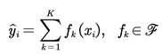
 is the CART space, q represents the structure of each tree, mapping samples to corresponding leaf nodes and T is the number of leaf nodes in the tree. Each fk corresponds to a tree whose leaf node weight is w.
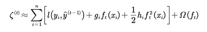
To learn the set of functions used in the model, it is necessary to minimize the objective function with a regularization term:
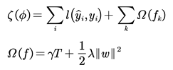
In Eq. (2), represents the predicted value of the model and represents the class label of the ith sample. The first term is the loss function and the second term is the regularizer, which is used to control the tree and avoid overfitting.
(2) Taylor expansion
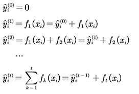
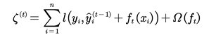
From Eq. (1), the prediction result of sample i after the tth iteration is known as:
A new function that minimizes the following objective function is introduced:
Then, the Taylor expansion is performed on the objective function in Eq. (4); the first three terms are taken and the high-order infinitesimal terms are removed. We arrived at:
 where and are the first and second derivatives of the loss function, respectively.
This does not affect the optimization of the function since is a constant in Eq. (5). By removing all the constant terms, the simplified objective function can be obtained:
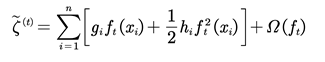
Only gi and hi need to be considered in Eq. (6), so the first and second derivatives of the loss function for each round can be calculated to obtain .
5.3. Evaluation Metrics
The confusion matrix is a very popular measure used to measure the performances of a classification models when solving classification problems. It achieves this through the calculation of performance metrics like accuracy, precision, recall and F1 scores. Figure 8 shows a binary-classification confusion matrix. The specific formulas and meanings thereof are shown in Table 3.
5.4. Results and Discussion
The proposed method was compared to three popular classifiers in the field of pattern recognition, such as Random forest (RF), Gradient Boosting Decision Tree (GBDT) and Support Vector Machine (SVM), that were also trained with the samples in Fig. 6. The results of each classifier are shown in Table 4. XGBoost visibly has an average accuracy of 89.34%, which is better than the 83.07% for RF, the 82.97% for GBDT and the 85.56% for SVM.
Although XGBoost has a high classification accuracy, its accuracy of track defect identification is still less than 90%. One reason for this may be that feature engineering limits the improvement of accuracy to some extent. Moreover, there are currently no stable parameter-tuning methods for some algorithms, and the best parameters are often selected through exhaustive methods, which adds uncertainty to model optimization.
6. ResNet-Based Defect Recognition Approaches for Ballastless Tracks
6.1. Convolutional Neural Network
A convolutional neural network (CNN) is a network architecture for deep learning [21] that learns directly from data. The concept was first introduced by postdoctoral Computer Science Researcher Yann LeCun. Notably, it has significant advantages in image segmentation, detection and classification. The overall CNN architecture includes an input layer, multiple alternating convolution and max-pooling layers, one fully connected layer and one classification layer, as shown in Figure 9.
The convolutional layer is the most important component of a CNN, since it is where most of the processing takes place. It requires input data, a filter and a feature map, among other things. The pooling layer simplifies output by performing non-linear downsampling and reducing the number of parameters that the network needs to learn. The fully connected layer conducts categorization based on the characteristics retrieved by the preceding layers and the filters applied to them. In addition to these three layers, there are two more important parameters: the dropout layer and the activation function.
6.2. Residual Neural Network
Previous CNN architectures were not able to scale to large numbers of layers, which resulted in limited performance. However, when more layers were added, a degradation problem was exposed: when the network depth increased, the accuracy would become saturated and then degrade rapidly.
To overcome this problem, a concept called residual learning building blocks was introduced for a deep residual learning framework [22]. In each block, input is split into two paths that are summed element-wise in the output. H(x) can be realized by feed-forward neural networks with shortcut connections. In terms of architecture, if any layer ends up damaging the performance of the model in a plain network, it will be skipped due to the presence of the skip connections. Residual neural networks (ResNets) are made by stacking these residual blocks together, as shown in Figure 10.
6.3. Receptive Field
In a fully connected layer, each neuron is affected by the whole of the input. In contrast, in a convolutional layer, each neuron has a strictly limited “field of view” (receptive field, or RF) [23,24,25]. The input of the layer outside of this field of view cannot alter the neuron’s activation. Within a convolutional layer, the spatial RF of a neuron is determined by its filter size: the larger the filter, the bigger the region of the input it can “see”. The filter size determines the RF of a convolutional layer based on layer input. In a CNN, RFn which is the size of a unit from layer n to the network input, can be calculated with:
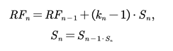 where Sn and kn are the stride and kernel size of layer n, respectively, and Sn is the cumulative stride from layer n to the input layer.
The receptive field size of a unit can be increased in a number of ways. One option is to stack more layers to make the network deeper, which will increase the receptive field size linearly, in theory, as each extra layer will increase the receptive field size by the kernel size. Subsampling, on the other hand, will increase the receptive field size multiplicatively.
In summary, the feature extraction of time-domain signals is more suitable for architecture with larger convolution kernels and fewer network layers. We have proposed a time-domain residual network that will expand the receptive field by stacking multi-layer convolution kernels with larger residual blocks near the input to increase the size of the receptive field and stacking several convolution kernels with smaller residual blocks in the back of the network to extract local and detailed features. Our calculations have shown that a large three-layer convolution kernel can obtain a receptive field size of 449×1 and a feature map size of 313×1, as shown in Figure 11.
6.4. Results and Discussion
The dataset was randomly divided into training and testing sets in a 3:1 ratio. To verify the impact of the receptive field on network performance, we tested the classification accuracy obtained with convolution kernels of different sizes. Global average pooling was used in the network. Instead of directly connecting the output to the Softmax layer, we adopted an architecture that was similar to GoogLeNet. In addition, we added dropout and fully connected layers and used L2 regularization to further suppress overfitting in the fully connected layers. The basic network architecture is shown in Figure 12.
The results thereof are shown in Table 5. A larger receptive field could be obtained when a larger convolution kernel was set. With a small convolution kernel, capturing low-frequency features with a large time-domain span was difficult and easily affected by high-frequency noise. On the other hand, the convolution kernel was not as large as it could have been. If the convolution kernel were too large, not only would the computational cost have increased but the accuracy would have decreased. Additionally, this would have increased the number of parameters and reduced the speed of the convergence of the network.
7. Conclusions
Under the impacts of long-term train load and the external environment, ballastless tracks have different degrees of damage and defectiveness, which poses a huge threat to the safety of railway operation. In this paper, according to the characteristics of the CRTSⅡ slab, research on DAS-technology-based defect identification in ballastless tracks was carried out, and the following conclusions were obtained:
(1) DAS equipment was installed and debugged to collect the vibration signals of trains and events along the line. Each track vibration signal was extracted by identifying the running train track, denoising, framing and labeling to build a defect dataset.
(2) Time–frequency-domain statistical features, the wavelet packet energy spectrum and the MFCCs of vibration signals were extracted to form a multi-dimensional vector. The XGBoost model was trained using the defect dataset and reached an accuracy of 89.34%. This model’s performance was better than that of other popular classifiers, such as RF, GBDT and SVM.
(3) A time-domain residual network that would expand the receptive field and test the accuracy obtained with convolution kernels of different sizes has been proposed. The best performance of this method can reach 94.82%, eliminating the manual process of feature extraction in traditional algorithms and realizing end-to-end information processing.
Author Contributions
All authors have read and agreed to the published version of the manu-script.
Funding
This work is supported by the Key Scientific and Technological Project Of Henan Province (No.222102210006) and the Science And Technology Development Project Of China Railway Design Corporation (No.2022A02538009).
Conflicts of Interest
The authors declare no conflict of interest regarding the publication of this research article.
References
- Ye X Y, Luo Y Y, Li Z W, et al. A Feasibility Analysis of the Infrared Thermography Technique in Surface Crack Detection for High-Speed Rail Slab Track. Mathematical Problems in Engineering 2023, 2023. [Google Scholar]
- Wang J, Lu C, Zhao Y. Reliability Assessment on Gap Height of Interface between CRTSⅡTrack Slab and CA Mortar. J. China Railway Soc 2023, 45, 117–125. [Google Scholar]
- Wu Y, Fu H, Bian X, et al. Impact of extreme climate and train traffic loads on the performance of high-speed railway geotechnical infrastructures. Journal of Zhejiang University-SCIENCE A 2023, 24, 189–205. [Google Scholar] [CrossRef]
- Liao H, Zhu Q, Zan Y, et al. Detection of ballastless track diseases in high-speed railway based on ground penetrating radar. Journal of Southwest Jiaotong University, 2016, 51(1).
- Guo Y, Liu G, Jing G, et al. Ballast fouling inspection and quantification with ground penetrating radar (GPR). International Journal of Rail Transportation 2023, 11, 151–168. [Google Scholar] [CrossRef]
- TAYLOR H F, LEE C E. Apparatus and method for fiber optic intrusion sensing: US, US 5194847[P].1993.
- Hu X, Tu Z, Zhou F, et al. A hydraulic fracture geometry inversion model based on distributed-acoustic-sensing data. SPE Journal 2023, 28, 1560–1576. [Google Scholar] [CrossRef]
- Liu J, Yuan S, Luo B, et al. Turning Telecommunication Fiber-Optic Cables into Distributed Acoustic Sensors for Vibration-Based Bridge Health Monitoring. Structural Control and Health Monitoring 2023, 2023. [Google Scholar]
- Mata Flores D, Sladen A, Ampuero J P, et al. Monitoring deep sea currents with seafloor distributed acoustic sensing. Earth and Space Science 2023, 10, e2022EA002723. [Google Scholar] [CrossRef]
- Wagner A, Nash A, Michelberger F, et al. The Effectiveness of Distributed Acoustic Sensing (DAS) for Broken Rail Detection. Energies 2023, 16, 522. [Google Scholar] [CrossRef]
- Yan B, Zhang K, Li H, et al. Acoustic Field Imaging of Pipeline Turbulence for Non-invasive and Distributed Gas Flow Measurement. IEEE Sensors Journal, 2023.
- Du X, Jia M, Huang S, et al. Event identification based on sample feature correction algorithm for Φ-OTDR. Measurement Science and Technology 2023, 34, 085120. [Google Scholar] [CrossRef]
- Lu Y, Zhu T, Chen L, et al. Distributed vibration sensor based on coherent detection of phase-OTDR. Journal of lightwave Technology 2010, 28, 3243–3249. [Google Scholar]
- Zinsou R, Liu X, Wang Y, et al. Recent progress in the performance enhancement of phase-sensitive OTDR vibration sensing systems. Sensors 2019, 19, 1709. [Google Scholar] [CrossRef]
- Peng F, Duan N, Rao Y J, et al. Real-time position and speed monitoring of trains using phase-sensitive OTDR. IEEE Photonics Technology Letters 2014, 26, 2055–2057. [Google Scholar] [CrossRef]
- He M, Feng L, Zhao D. Application of distributed acoustic sensor technology in train running condition monitoring of the heavy-haul railway. Optik 2019, 181, 343–350. [Google Scholar] [CrossRef]
- Otsu, N. A threshold selection method from gray-level histograms. IEEE transactions on systems, man, and cybernetics 1979, 9, 62–66. [Google Scholar] [CrossRef]
- Tabjula J, Sharma J. Feature extraction techniques for noisy distributed acoustic sensor data acquired in a wellbore. Applied Optics 2023, 62, E51–E61. [Google Scholar] [CrossRef] [PubMed]
- Mata Flores D, Mercerat E D, Ampuero J P, et al. Identification of two vibration regimes of underwater fibre optic cables by Distributed Acoustic Sensing. Geophysical Journal International 2023, 234, 1389–1400. [Google Scholar] [CrossRef]
- Chen T, Guestrin C. Xgboost: A scalable tree boosting system[C]//Proceedings of the 22nd acm sigkdd international conference on knowledge discovery and data mining. 2016: 785-794.
- LeCun Y, Kavukcuoglu K, Farabet C. Convolutional networks and applications in vision[C]//Proceedings of 2010 IEEE international symposium on circuits and systems. IEEE, 2010: 253-256.
- He K, Zhang X, Ren S, et al. Deep residual learning for image recognition[C]//Proceedings of the IEEE conference on computer vision and pattern recognition. 2016: 770-778.
- Araujo A, Norris W, Sim J. Computing receptive fields of convolutional neural networks. Distill 2019, 4, e21. [Google Scholar]
- Understanding the Effective Receptive Field in Deep Convolutional Neural Networks.
- The Receptive Field as a Regularizer in Deep Convolutional Neural Networks for Acoustic Scene Classification.
Figure 1.
CRTSII slab defects.
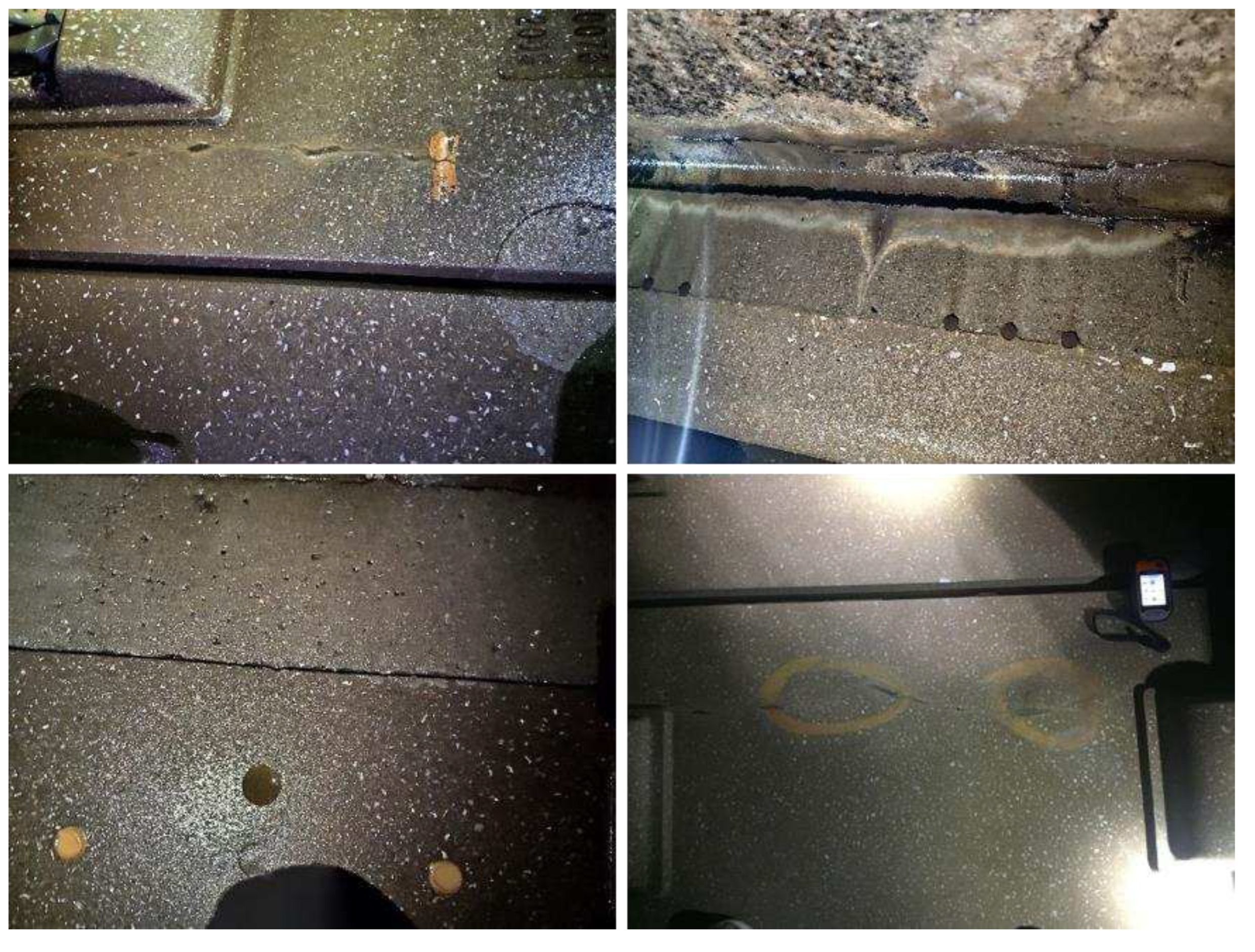
Figure 2.
Existing optical fiber cable used by sensing.
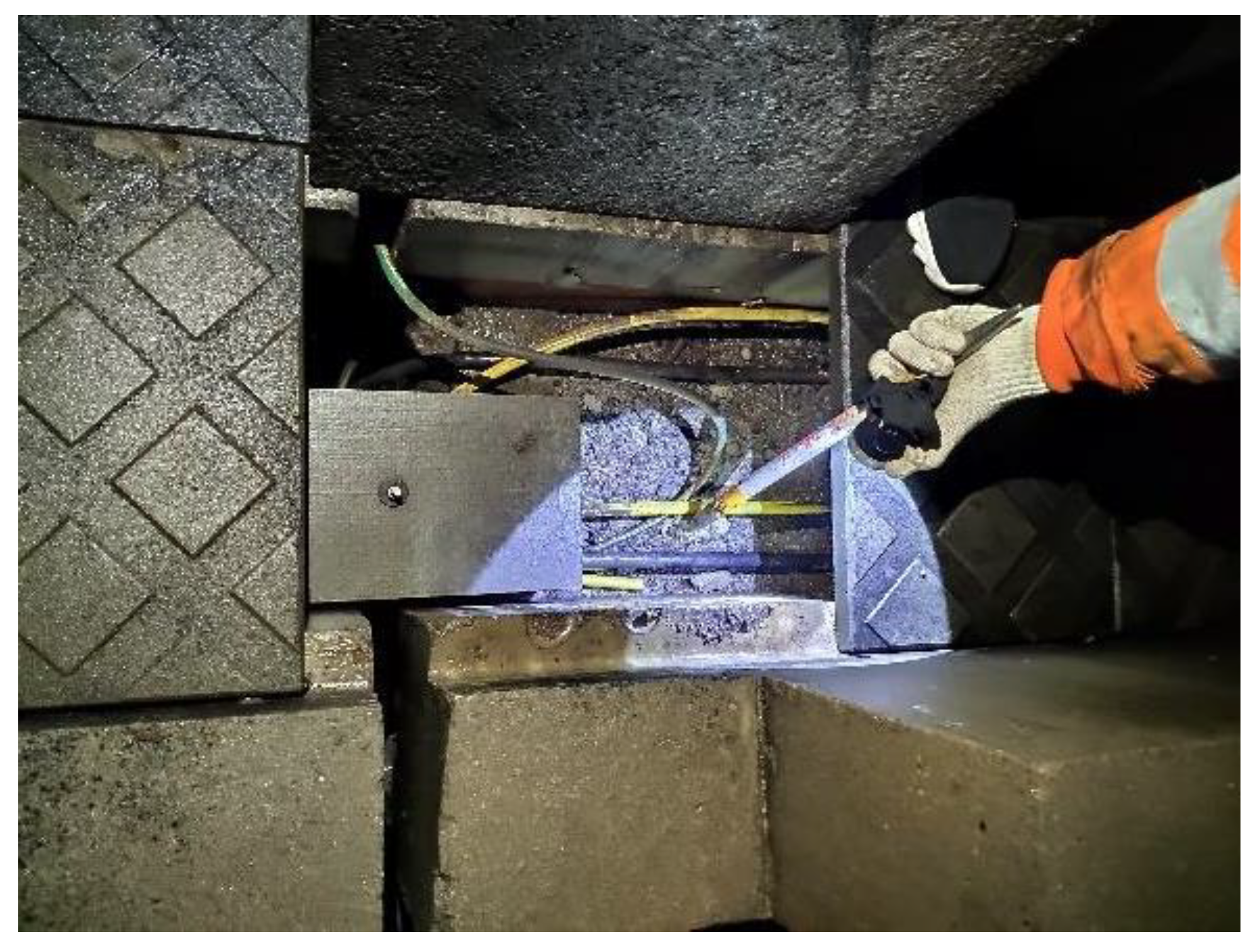
Figure 3.
Original signal.
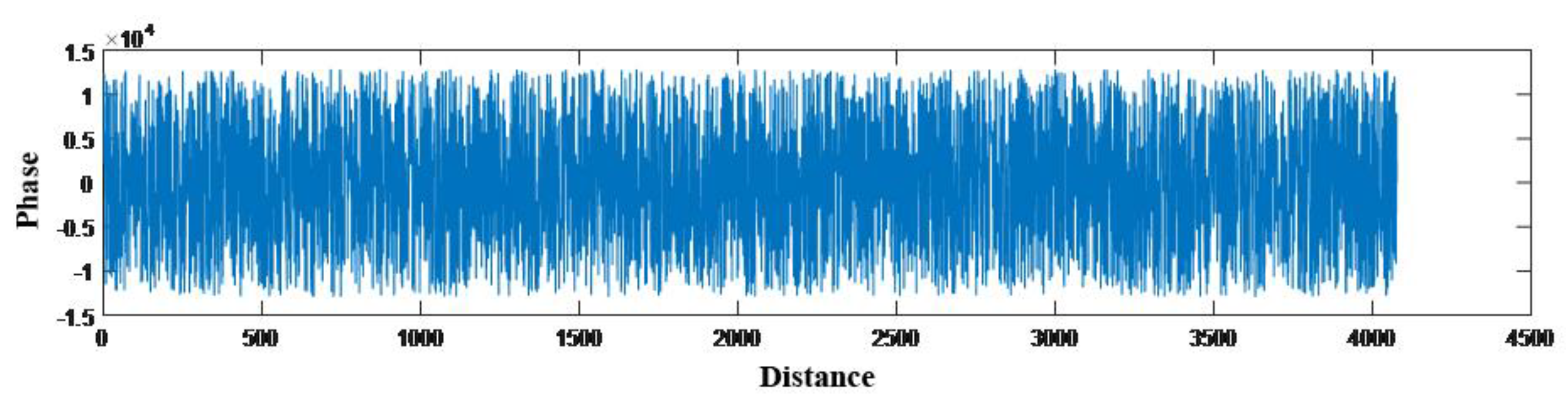
Figure 4.
Smoothing results of different times.
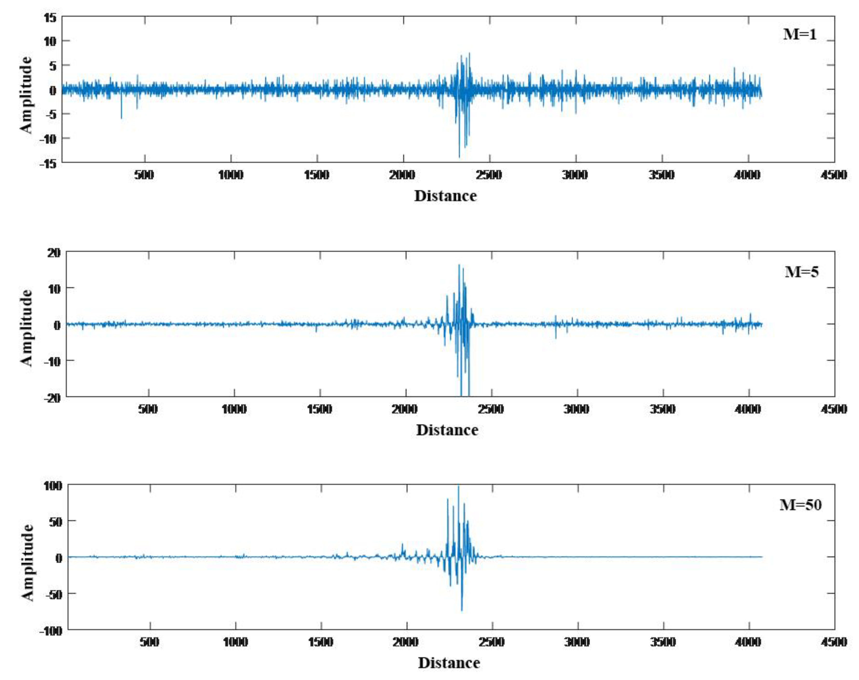
Figure 5.
Train movement trajectory.
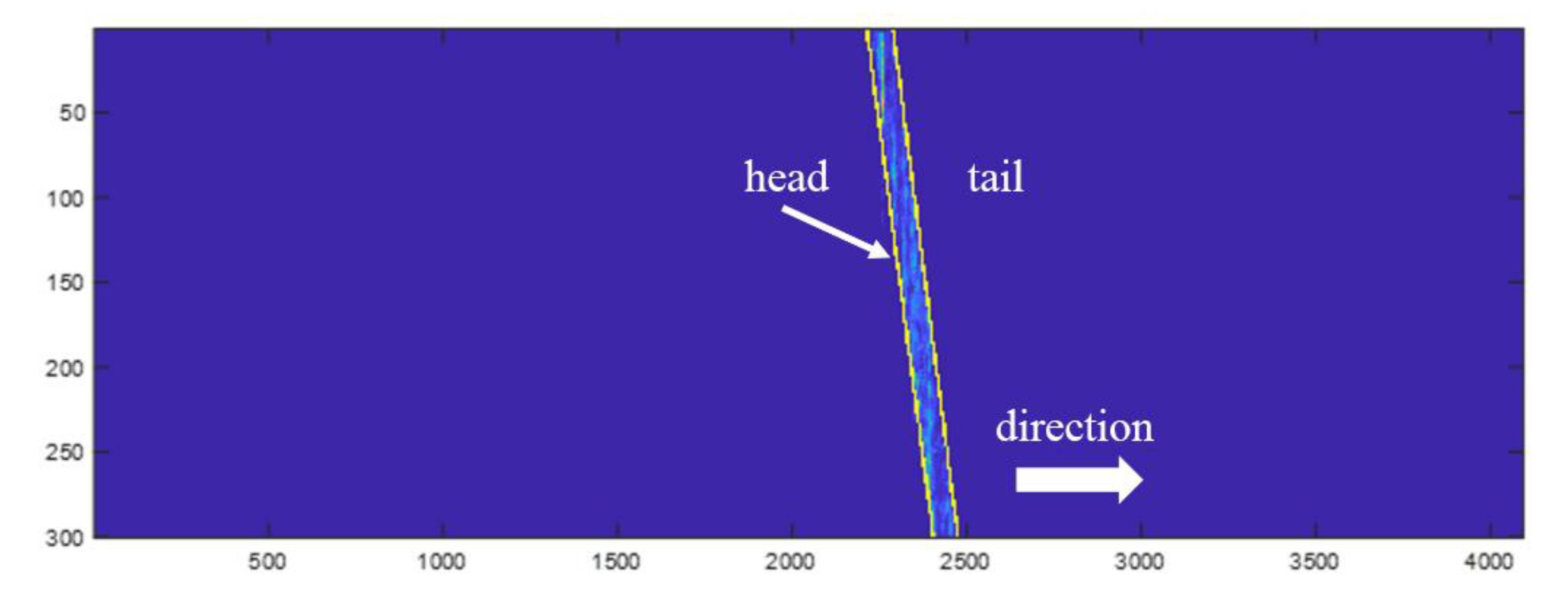
Figure 6.
The scale of six samples in dataset.
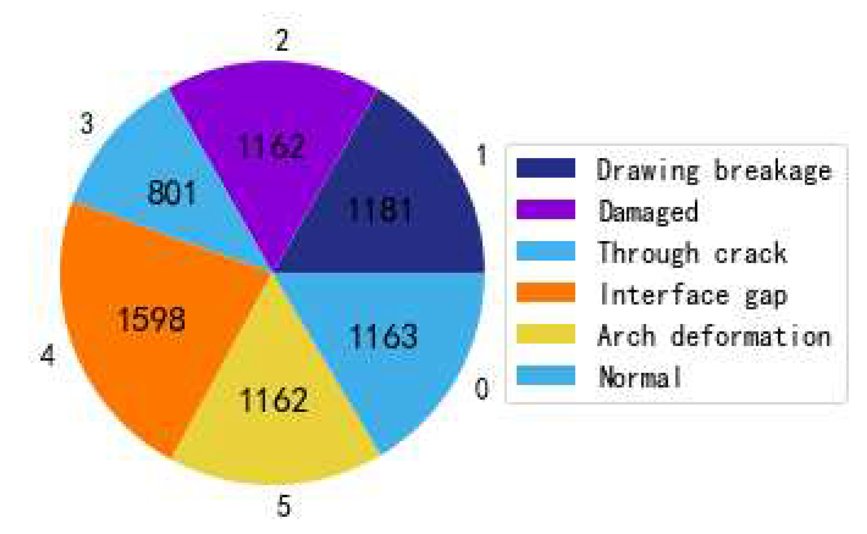
Figure 7.
Data sample: a) Original phase; b) Differenced phase; c) Frequency spectrum of differenced phase.
Figure 7.
Data sample: a) Original phase; b) Differenced phase; c) Frequency spectrum of differenced phase.
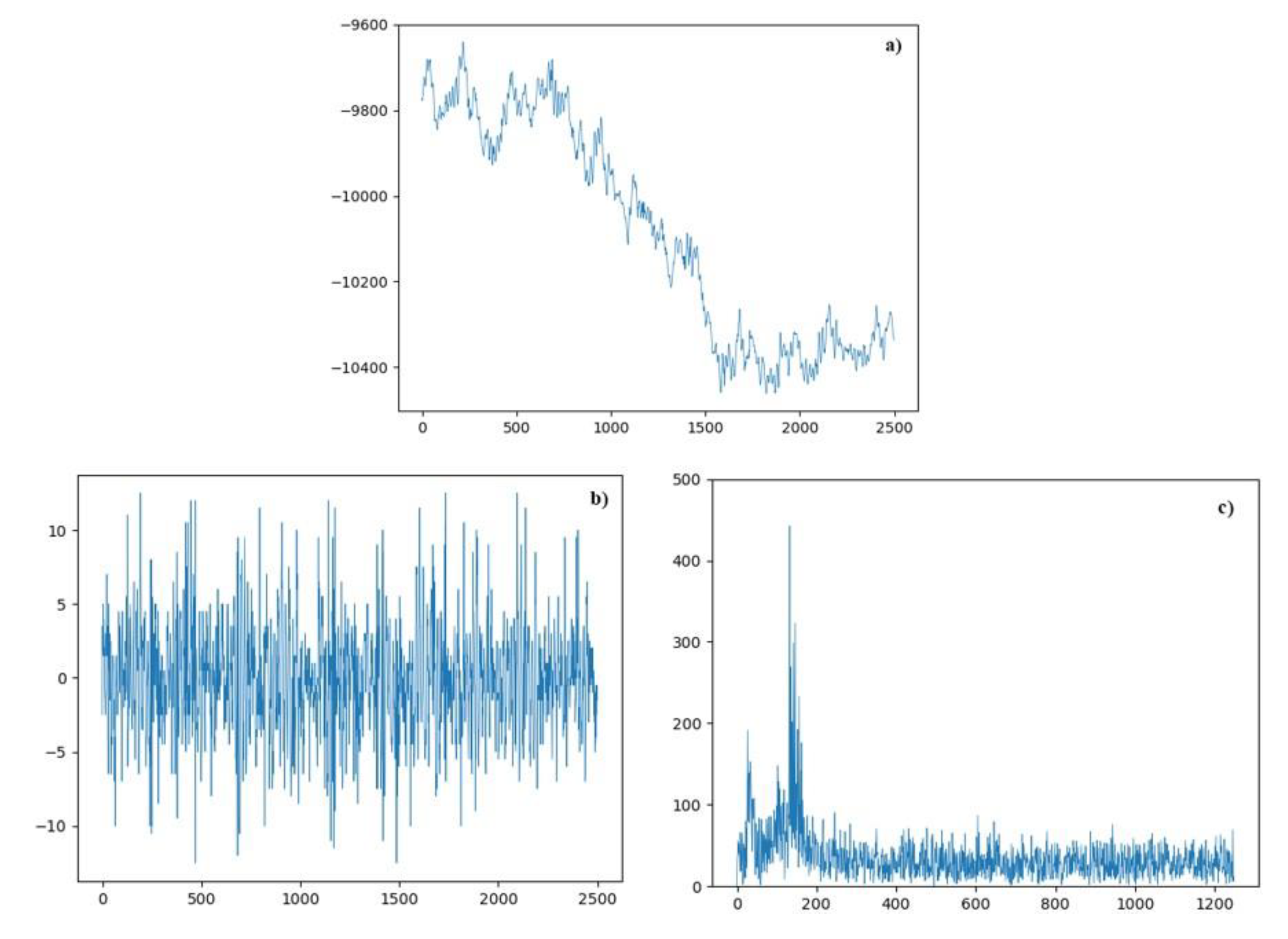
Figure 8.
Binary classification confusion matrix.
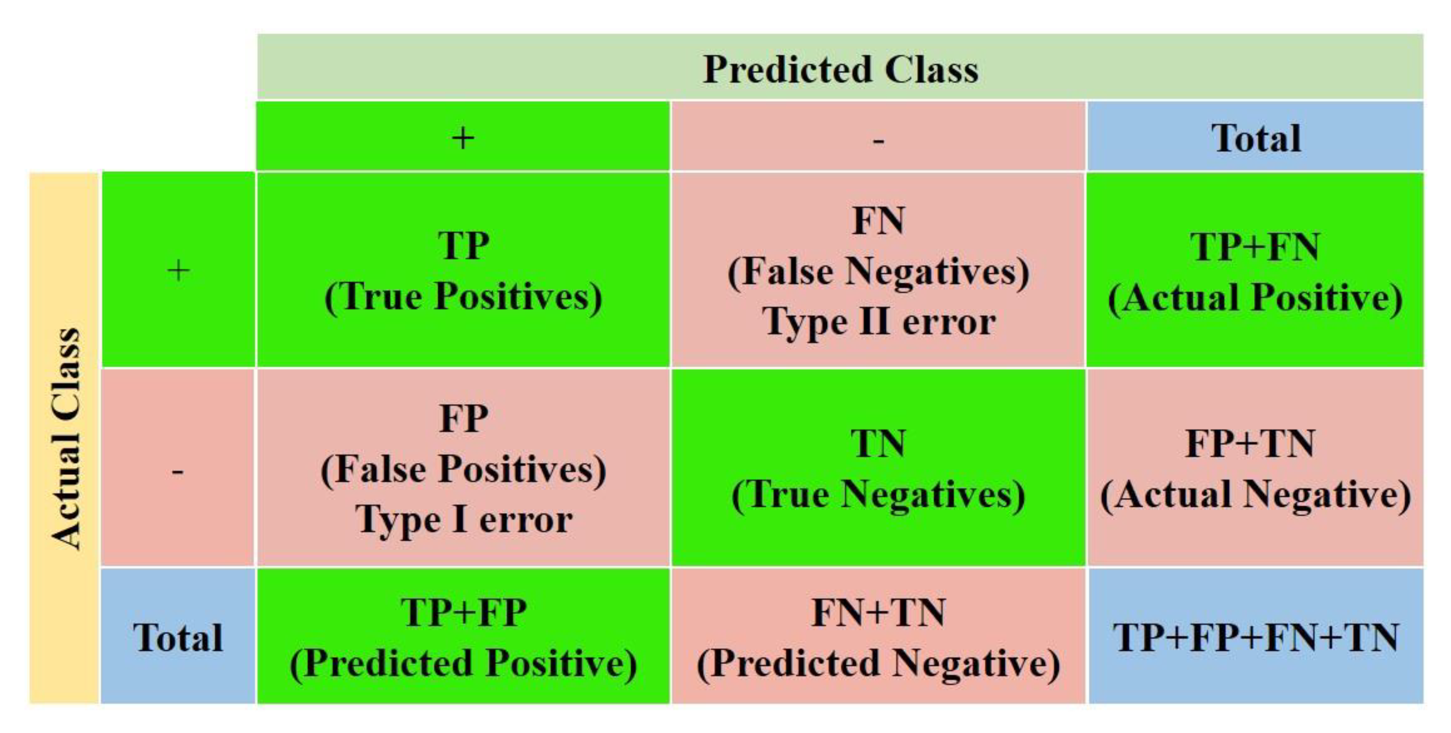
Figure 9.
Convolutional Neural Network Architecture.
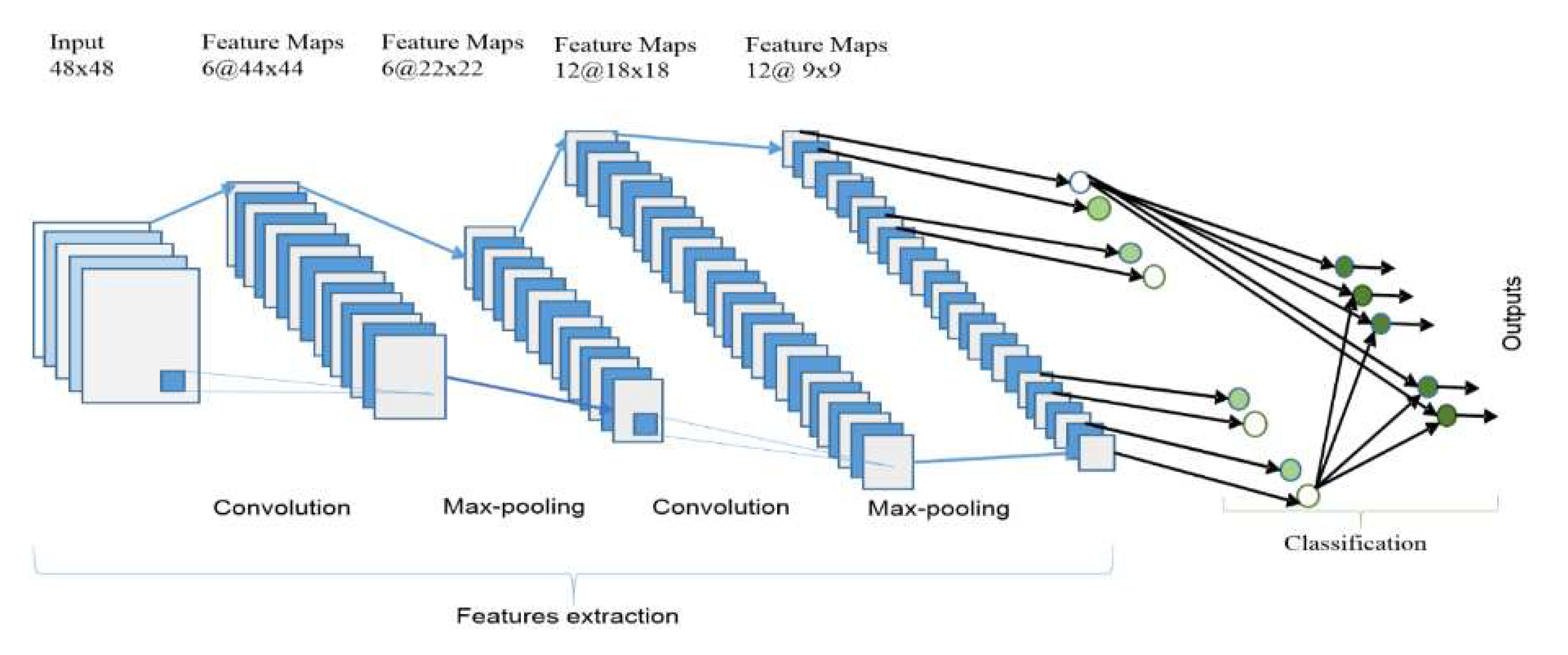
Figure 10.
ResNets Architecture.
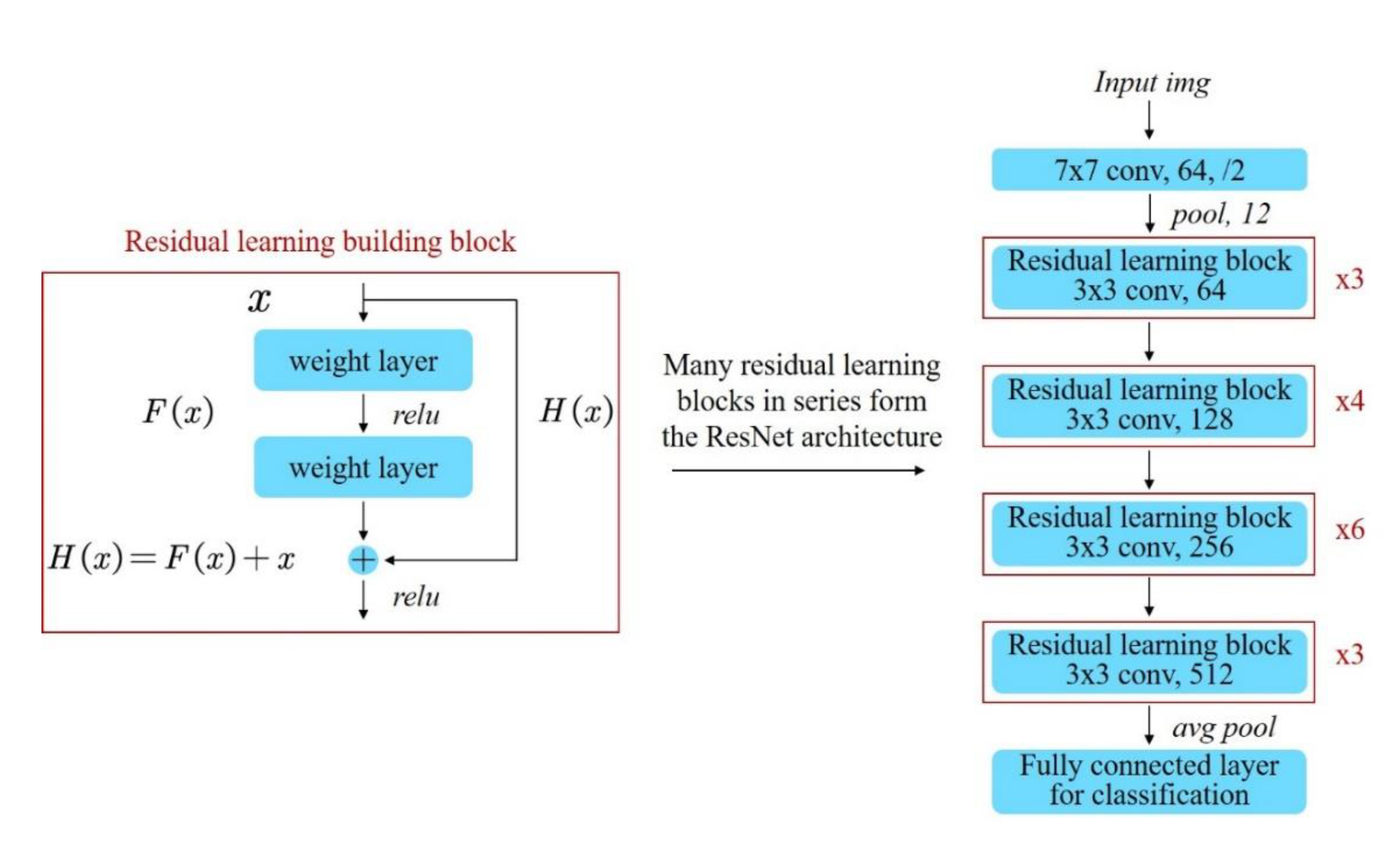
Figure 11.
The module of increased receptive field.
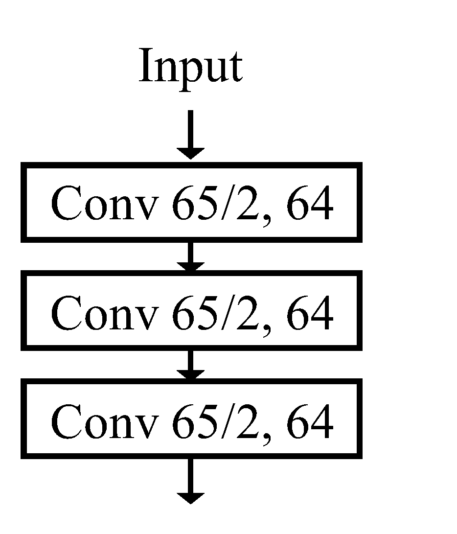
Figure 12.
1D-ResNet with increased receptive field.
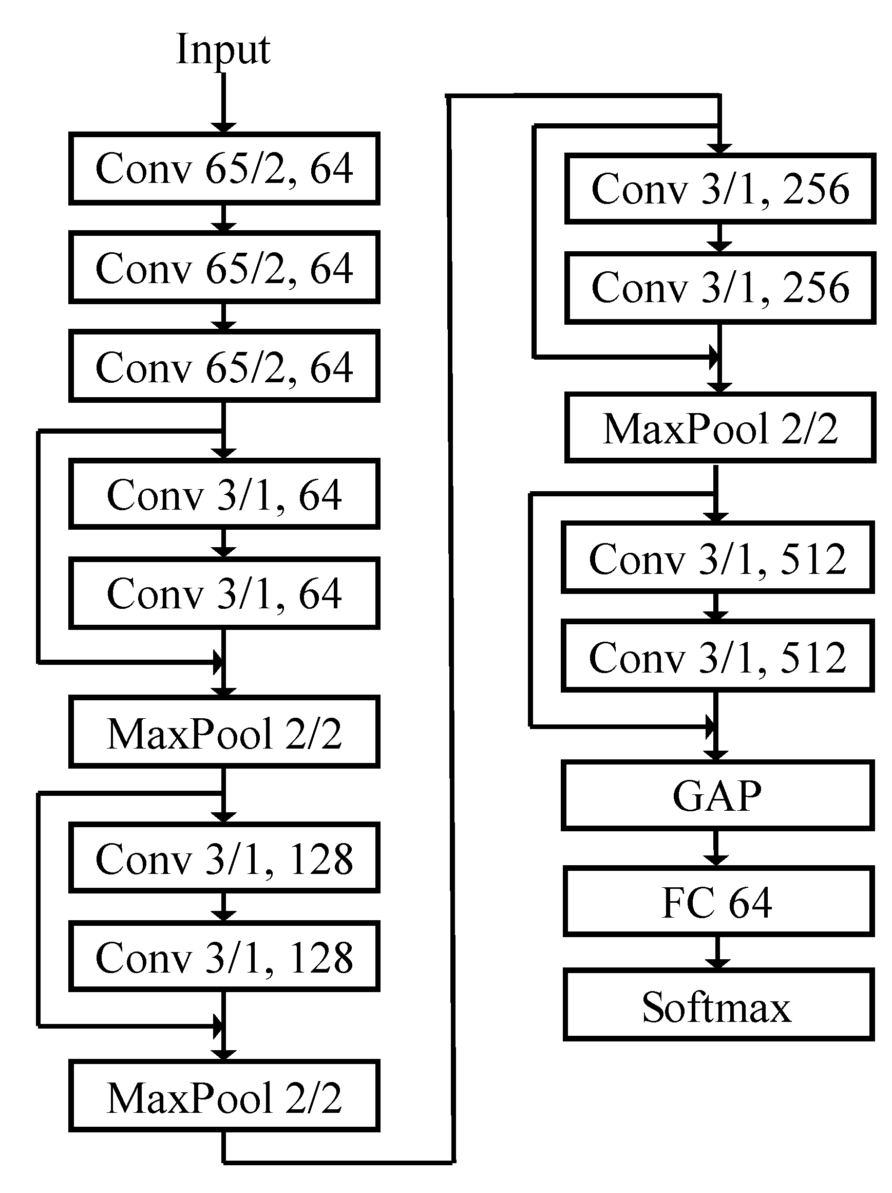

Table 1.
The key parameters of equipment.
| Name | Value | Unit |
|---|---|---|
| Spatial resolution | 6.4 | m |
| Track slab length | 6.45 | m |
| Pulse duration | 64 | ns |
| Sampling rate | 2564 | Hz |
Table 2.
The extracted features for each frame.
| Domain | Feature Description | Number |
|---|---|---|
| Time | Average amplitude, Standard deviation, Zero crossing rate, Root mean square, Skewness, Kurtosis | 6 |
| Frequency | Average amplitude, Standard deviation, Skewness, Kurtosis, Spectral entropy, Spectral centroid | 6 |
| Wavelet packet | Wavelet packet energy spectra | 8 |
| Mel scale | Mel-Frequency Cepstral Coefficients | 13 |
| Total | 33 |
Table 3.
Standard performance metrics of the classifier.
| Name | Formula | Meaning |
|---|---|---|
| Accuracy | (TP+TN)/(TP+FP+TN+FN) | It simply measures how often the classifier makes the correct prediction. |
| Precision | TP/(TP+FP) | It is a measure of correctness that is achieved in true prediction. |
| Recall | TP/(TP+FN) | It is a measure of actual observations which are predicted correctly, i.e. how many observations of positive class are actually predicted as positive. |
| F1-score | (2*TP)/(2*TP+FP+FN) | It is a number between 0 and 1 and is the harmonic mean of precision and recall. |
Table 4.
Performance of four classifiers.
| Label | Precision | Recall | F1-Score | |
|---|---|---|---|---|
| RF Accuracy=0.8307 |
0 | 0.8772 | 0.8152 | 0.8451 |
| 1 | 0.7368 | 0.7456 | 0.7412 | |
| 2 | 0.8365 | 0.8365 | 0.8365 | |
| 3 | 0.8606 | 0.8404 | 0.8504 | |
| 4 | 0.7198 | 0.7661 | 0.7422 | |
| 5 | 0.9583 | 0.9877 | 0.9728 | |
| GBDT Accuracy=0.8297 |
0 | 0.8508 | 0.8370 | 0.8438 |
| 1 | 0.7321 | 0.7278 | 0.7300 | |
| 2 | 0.8713 | 0.8462 | 0.8585 | |
| 3 | 0.8679 | 0.8638 | 0.8659 | |
| 4 | 0.7126 | 0.7251 | 0.7188 | |
| 5 | 0.9524 | 0.9816 | 0.9668 | |
| XGBoost Accuracy=0.8934 |
0 | 0.8636 | 0.9293 | 0.8953 |
| 1 | 0.8485 | 0.8284 | 0.8383 | |
| 2 | 0.9500 | 0.9135 | 0.9314 | |
| 3 | 0.9238 | 0.9108 | 0.9173 | |
| 4 | 0.8225 | 0.8129 | 0.8176 | |
| 5 | 0.9753 | 0.9693 | 0.9723 | |
| SVM Accuracy=0.8556 |
0 | 0.8595 | 0.8641 | 0.8618 |
| 1 | 0.7938 | 0.7515 | 0.7720 | |
| 2 | 0.8738 | 0.8654 | 0.8696 | |
| 3 | 0.8952 | 0.8826 | 0.8889 | |
| 4 | 0.7459 | 0.7895 | 0.7670 | |
| 5 | 0.9697 | 0.9816 | 0.9756 |
Table 5.
Various kernel sizes and impacts on classification.
| Kernel sizes | Accuracy | Loss | Parameters | Output RF |
|---|---|---|---|---|
| 129/2, 64 | 0.9157 | 0.3140 | 2.86M | 897 |
| 65/2, 64 | 0.9482 | 0.2061 | 2.33M | 449 |
| 33/2, 64 | 0.9414 | 0.2337 | 2.06M | 225 |
| 17/2, 64 | 0.9249 | 0.2803 | 1.93M | 113 |
| 11/2, 64 | 0.9068 | 0.3423 | 1.88M | 71 |
Disclaimer/Publisher’s Note: The statements, opinions and data contained in all publications are solely those of the individual author(s) and contributor(s) and not of MDPI and/or the editor(s). MDPI and/or the editor(s) disclaim responsibility for any injury to people or property resulting from any ideas, methods, instructions or products referred to in the content. |
© 2023 by the authors. Licensee MDPI, Basel, Switzerland. This article is an open access article distributed under the terms and conditions of the Creative Commons Attribution (CC BY) license (http://creativecommons.org/licenses/by/4.0/).
Copyright: This open access article is published under a Creative Commons CC BY 4.0 license, which permit the free download, distribution, and reuse, provided that the author and preprint are cited in any reuse.


