Submitted:
29 July 2023
Posted:
02 August 2023
Read the latest preprint version here
Abstract
Generative artificial intelligence (GenAI) has been developing with many incredible achievements like ChatGPT and Bard. Deep generative model (DGM) is a branch of GenAI, which is preeminent in generating raster data such as image and sound due to strong points of deep neural network (DNN) in inference and recognition. The built-in inference mechanism of DNN, which simulates and aims to synaptic plasticity of human neuron network, fosters generation ability of DGM which produces surprised results with support of statistical flexibility. Two popular approaches in DGM are Variational Autoencoders (VAE) and Generative Adversarial Network (GAN). Both VAE and GAN have their own strong points although they share and imply underline theory of statistics as well as incredible complex via hidden layers of DNN when DNN becomes effective encoding/decoding functions without concrete specifications. In this research, I try to unify VAE and GAN into a consistent and consolidated model called Adversarial Variational Autoencoders (AVA) in which VAE and GAN complement each other, for instance, VAE is good at generator by encoding data via excellent ideology of Kullback-Leibler divergence and GAN is a significantly important method to assess reliability of data which is realistic or fake. In other words, AVA aims to improve accuracy of generative models, besides AVA extends function of simple generative models. In methodology this research focuses on combination of applied mathematical concepts and skillful techniques of computer programming in order to implement and solve complicated problems as simply as possible.
Keywords:
deep generative model (DGM)
; Variational Autoencoders (VAE)
; Generative Adversarial Network (GAN)
1. Introduction
Variational Autoencoders (VAE) and Generative Adversarial Network (GAN) are two popular approaches for developing deep generative model with support of deep neural network (DNN) where high capacity of DNN contributes significantly to successes of GAN and VAE. There are some researches which combined VAE and GAN. Larsen et al. (Larsen, Sønderby, Larochelle, & Winther, 2016) proposed a traditional combination of VAE and GAN by considering decoder of VAE as generator of GAN (Larsen, Sønderby, Larochelle, & Winther, 2016, p. 1558). They constructed target optimization function as sum of likelihood function of VAE and target function of GAN (Larsen, Sønderby, Larochelle, & Winther, 2016, p. 1560). This research is similar to their research (Larsen, Sønderby, Larochelle, & Winther, 2016, p. 1561) except that the construction optimization functions in two researches are slightly different where the one in this research does not include target function of GAN according to traditional approach of GAN. However uncorrelated variables will be removed after gradients are determined. Moreover, because encoded data z is basically randomized in this research, I do not make a new random z’ to be included into target function of GAN. This research also mentions skillful techniques of derivatives in backpropagation algorithm.
Mescheder et al. (Mescheder, Nowozin, & Geiger, 2017) transformed gain function of VAE including Kullback-Leibler divergence into gain function of GAN via a so-called real-valued discrimination network (Mescheder, Nowozin, & Geiger, 2017, p. 2394) related to Nash equilibrium equation and sigmoid function and then, they trained the transformed VAE by stochastic gradient descent method. Actually, they estimated three parameters (Mescheder, Nowozin, & Geiger, 2017, p. 2395) like this research, but their method focused on mathematical transformation while I focus on skillful techniques in implementation. In other words, Mescheder et al. (Mescheder, Nowozin, & Geiger, 2017) tried to fuse VAE into GAN whereas I combine them by mutual and balancing way but both of us try to make unification of VAE and GAN. Rosca et al. (Rosca, Lakshminarayanan, Warde-Farley, & Mohamed, 2017, p. 4) used a density ratio trick to convert Kullback-Leibler divergence of VAE into the mathematical form log(x / (1–x)) which is similar to GAN target function log(x) + log(1–x). Actually, they made a fusion of VAE and GAN like Mescheder et al. did. The essence of their methods is based on convergence of Nash equilibrium equation. Ahmad et al. combined VAE and GAN separately as featured experimental research. Firstly, they trained VAE and swapped encoder-decoder network to decoder-encoder network so that output of VAE becomes some useful information which in turn becomes input of GAN instead that GAN uses random information as input as usual (Ahmad, Sun, You, Palade, & Mao, 2022, p. 6). Miolane et al. (Miolane, Poitevin, & Li, 2020) combined VAE and GAN by summing target functions of VAE and GAN weighted with regular hyperparameters (Miolane, Poitevin, & Li, 2020, p. 974). Later, they first trained VAE and then sent output of VAE to input of GAN (Miolane, Poitevin, & Li, 2020, p. 975).
In general, this research focuses on incorporating GAN into VAE by skillful techniques related to both stochastic gradient descent and software engineering architecture, which neither focuses on purely mathematical fusion nor focuses on experimental tasks. In practice, many complex mathematical problems can be solved effectively by some skillful techniques of computer programming. Moreover, the proposed model called Adversarial Variational Autoencoders (AVA) aims to extend functions of VAE and GAN as a general architecture for generative model. For instance, AVA will provide encoding function that GAN does not concern and provide discrimination function that VAE needs to distinguish fake data from realistic data. The corporation of VAE and GAN in AVA is strengthened by regular and balance mechanism, which obviously, is natural and like fusion mechanism. In some cases, it is better than fusion mechanism because both built-in VAE and GAN inside AVA can uphold their own strong features. Therefore, experiment in this research is not too serious with large data when I only compare AVA and VAE within small dataset, which aims to prove the proposed method mentioned in the next section.
2. Methodology
In this research I propose a method as well as a generative model which incorporate Generative Adversarial Network (GAN) into Variational Autoencoders (VAE) for extending and improving deep generative model because GAN does not concern how to code original data and VAE lacks mechanisms to assess quality of generated data with note that data coding is necessary to some essential applications such as image impression and recognition whereas audit quality can improve accuracy of generated data. As a convention, let vector variable x = (x1, x2,…, xm)T and vector variable z = (z1, z2,…, zn)T be original data and encoded data whose dimensions are m and n (m > n), respectively. A generative model is represented by a function f(x | Θ) = z, f(x | Θ) ≈ z, or f(x | Θ) → z where f(x | Θ) is implemented by a deep neural network (DNN) whose weights are Θ, which converts the original data x to the encoded data z and is called encoder in VAE. A decoder in VAE which converts expectedly the encoded data z back to the original data is represented by a function g(z | Φ) = x’ where g(z | Φ) is also implemented by a DNN whose weights are Φ with expectation that the decoded data x’ is approximated to the original data x as x’ ≈ x. The essence of VAE is to minimize the following loss function for estimating the encoded parameter Θ and the decoded parameter Φ.
Such that:
Note that ||x – x’|| is Euclidean distance between x and x’ whereas KL(μ(x), Σ(x) | N(0, I)) is Kullback-Leibler divergence between Gaussian distribution of x whose mean vector and covariance matrix are μ(x) and Σ(x) and standard Gaussian distribution N(0, I) whose mean vector and covariance matrix are 0 and identity matrix I.
GAN does not concern the encoder f(x | Θ) = z but it focuses on optimizing the decoder g(z | Φ) = x’ by introducing a so-called discriminator which is a discrimination function d(x | Ψ): x → [0, 1] from concerned data x or x’ to range [0, 1] in which d(x | Ψ) can distinguish fake data from real data. In other words, the larger result the discriminator d(x’ | Ψ) derives, the more realistic the generated data x’ is. Obviously, d(x | Ψ) is implemented by a DNN whose weights are Ψ with note that this DNN has only one output neuron denoted d0. The essence of GAN is to optimize mutually the following target function for estimating the decoder parameter Φ and the discriminator parameter Ψ.
Such that Φ and Ψ are optimized mutually as follows:
The proposed generative model in this research is called Adversarial Variational Autoencoders (AVA) because it combines VAE and GAN by fusing mechanism in which loss function and balance function are optimized parallelly. The AVA loss function implies loss information in encoder f(x | Θ), decoder g(z | Φ), discriminator d(x | Ψ) as follows:
The balance function of AVA is to supervise the decoding mechanism, which is the GAN target function as follows:
The key point of AVA is that the discriminator function occurs in both loss function and balance function via the expression log(1 – d(g(z | Φ) | Ψ)), which means that the capacity of how to distinguish fake data from realistic data by discriminator function affects the decoder DNN. As a result, the three parameters Θ, Φ, and Ψ are optimized mutually according to both loss function and balance function as follows:
Because the encoder parameter Θ is independent from both the decoder parameter Φ and the discriminator parameter Ψ, its estimate is specified as follows:
Because the decoder parameter Φ is independent from the encoder parameter Θ, its estimate is specified as follows:
Note that the Euclidean distance ||x – x’|| is only dependent on Θ. Because the discriminator tries to increase credible degree of realistic data and decrease credible degree of fate data, its parameter Ψ has following estimate:
By applying stochastic gradient descent (SDG) algorithm into backpropagation algorithm, these estimates are determined based on gradients of loss function and balance function as follows:
where γ (0 < γ ≤ 1) is learning rate. Let af(.), ag(.), and ad(.) be activation functions of encoder DNN, decoder DNN, and discriminator DNN, respectively and so, let af’(.), ag’(.), and ad’(.) be derivatives of these activation functions, respectively. The encoder gradient regarding Θ is (Doersch, 2016, p. 9):
The decoder gradient regarding Φ is:
where,
The discriminator gradient regarding Ψ is:
As a result, SGD algorithm incorporated into backpropagation algorithm for solving AVA is totally determined as follows:
where notation [i] denotes the ith element in vector. Please pay attention to the derivatives af’(.), ag’(.), and ad’(.) because they are helpful techniques to consolidate AVA. The reason of two different occurrences of derivatives ad’(d(x’ | Ψ*)) and ag’(x’) in decoder gradient regarding Φ is nontrivial because the unique output neuron of discriminator DNN is considered as effect of the output layer of all output neurons in decoder DNN.
Figure 1.
Causality effect relationship between decoder DNN and discriminator DNN.
When weights are assumed to be 1, error of causal decoder neuron is error of discriminator neuron multiplied with derivative at the decoder neuron and moreover, the error of discriminator neuron, in turn, is product of its minus bias –d’(.) and its derivative a’d(.).
It is necessary to describe AVA architecture because skillful techniques cannot be applied into AVA without clear and solid architecture. The key point to incorporate GAN into VAE is that the error of generated data is included in both decoder and discriminator, besides decoded data x’ which is output of decoder DNN becomes input of discriminator DNN.
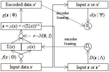
Figure 2 shows the AVA architecture.
AVA architecture follows an important aspect of VAE where the encoder f(x | Θ) does not produce directly decoded data z as f(x | Θ) = z. It actually produces mean vector μ(x) and covariance matrix Σ(x) belonging to x instead. In this research, μ(x) and Σ(x) are flatten into an array of neurons output layer of the encoder f(x | Θ).
The actual decoded data z is calculated randomly from μ(x) and Σ(x) along with a random vector r.
where r follows standard Gaussian distribution with mean vector 0 and identity covariance matrix I and each element of (Σ(x))1/2 is squared root of the corresponding element of Σ(x). This is an excellent invention in traditional literature which made the calculation of Kullback-Leibler divergence much easier without loss of information.
The balance function bAVA(Φ, Ψ) aims to balance decoding task and discrimination task without partiality but it can lean forward decoding task for improving accuracy of decoder by including the error of original data x and decoded data x’ into balance function as follows:
As a result, the estimate of discriminator parameter Ψ is:
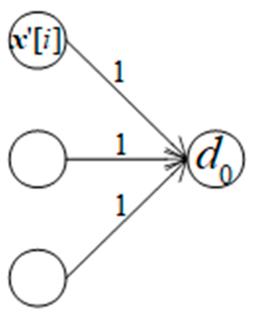
In a reverse causality effect relationship in which the unique output neuron of discriminator DNN is cause of all output neurons of decoder DNN as shown in Figure 3.
Figure 3.
Reverse causality effect relationship between discriminator DNN and decoder DNN.

Suppose bias of each decoder output neuron is bias[i], error of the discriminator output neuron error[i] is sum of weighted biases which is in turn multiplied with derivative at the discriminator output neuron with note that every weighted bias is also multiplied with derivative at every decoder output neuron. Suppose all weights are 1, we have:
Because the balance function bAVA(Φ, Ψ) aims to improve the decoder g(z | Φ), it is possible to improve the encoder f(x | Θ) by similar technique with note that output of encoder is mean vector μ(x) and covariance matrix Σ(x). In this research, I propose another balance function BAVA(Θ, Λ) to assess reliability of the mean vector μ(x) because μ(x) is most important to randomize z and μ(x) is linear. Let D(μ(x) | Λ) be discrimination function for encoder DNN from μ(x) to range [0, 1] in which D(μ(x) | Λ) can distinguish fake mean μ(x) from real mean μ(x’). Obviously, D(μ(x) | Λ) is implemented by a so-called encoding discriminator DNN whose weights are Λ with note that this DNN has only one output neuron denoted D0. The balance function BAVA(Θ, Λ) is specified as follows:
Note,
AVA loss function is modified with regard to the balance function BAVA(Θ, Λ) as follows:
By similar way of applying SGD algorithm, it is easy to estimate the encoding discriminator parameter Λ as follows:
where aD(.) and a’D(.) are activation function of the discriminator D(μ(x) | Λ) and its derivative, respectively.
The encoder parameter Θ is consisted of two separated parts Θμ and ΘΣ because the output of encoder f(x | Θ) is consisted of mean vector μ(x) and covariance matrix Σ(x).
When the balance function BAVA(Θ, Λ) is included in AVA loss function, the part Θμ is recalculated whereas the part ΘΣ is kept intact as follows:
Figure 4 shows AVA architecture with support of assessing encoder.
Similarly, the balance function BAVA(Φ, Λ) can lean forward encoding task for improving accuracy of encoder f(x | Θ) by concerning the error of original mean μ(x) and decoded data mean μ(x’) as follows:
Without repeating explanations, the estimate of discriminator parameter Λ is modified as follows:
These variants of AVA are summarized, and their tests are described in the next section.
3. Experimental results and discussions
In this experiment, AVA is tested with VAE but there are 5 versions of AVA such as AVA1, AVA2, AVA3, AVA4, and AVA5. Recall that AVA1 is normal version of AVA whose parameters are listed as follows:
AVA2 leans forward improving accuracy of decoder DNN by modifying discriminator parameter Ψ as follows:
AVA3 supports the balance function BAVA(Θ, Λ) for assessing reliability of encoder f(x | Θ). Its parameters are listed as follows:
AVA4 is a variant of AVA3 along with leaning forward improving accuracy of encoder f(x | Θ) like AVA2. Its parameters are listed as follows:
AVA5 is the last one which supports all functions such as decoder supervising, leaning decoder, encoder supervising, and learning encoder.
The experiment is performed on a laptop with CPU AMD64 4 processors, 4GB RAM, Windows 10, and Java 15. The dataset is a set of ten 180x250 images, but convolution layers built in AVA zoom out 3 times smaller due to lack of memory. The four AVA variants will be evaluated by root mean square error (RMSE) with 19 learning rates γ = 1, 0.9,…, 0.1, 0.09, 0.001 because stochastic gradient descent (SGD) algorithm is affected by learning rate and the accuracy of AVA varies a little bit within a learning rate because of randomizing encoded data z in VAE algorithm. Given an AVA was trained by 10 images in the dataset, let imageBest be the best image generated by such AVA, which is compared with the ith image denoted images[i] in dataset and then, RMSE of such AVA and the ith image is calculated as follows:
The overall RMSE of such AVA is average RMSE over N=10 test images as follows:
This means:
Where N is the number of images, N=10 and ni is the number of pixels of the ith image. Obviously, image[i][j] (imageBest[j]) is the jth pixel of the ith image (the best image). The notation ||.|| denotes norm of pixel. For example, norm of RGB pixel is where r, g, and b are red color, green color, and blue color of such pixel. The smaller the RMSE is, the better the AVA is. Table 1 shows RMSE values of AVA1, AVA2, AVA3, AVA4, AVA5, and VAE with 10 learning rates γ = 1, 0.9, 0.8,…, 0.1.
Table 1 shows RMSE values of AVA1, AVA2, AVA3, AVA4, AVA5, and VAE with 9 learning rates γ = 0.09, 0.08,…, 0.01.
From experimental results shown in Table 1 and Table 2, RMSE means of AVA1, AVA2, AVA3, AVA4, AVA5, are VAE over all learning rates are 0.1787, 0.1786, 0.1783, 0.1783, 0.1783, and 0.2454, respectively. Because AVA3, AVA4, and AVA5 result the same best RMSE (0.1783), it is asserted that AVA with any discriminators in regardless of decoder discriminator (AVA5) or encoder discriminator (AVA3, AVA4, AVA5) but it seems that encoder discriminator is better than traditional decoder discriminator, for instance, Larsen et al. (Larsen, Sønderby, Larochelle, & Winther, 2016) focused on decoder discriminator. Therefore, we check again RMSE standard deviations of AVA1, AVA2, AVA3, AVA4, AVA5, and VAE which are 0.0028, 0.0017, 0.0019, 0.0011, 0.0012, and 0.0054, respectively. AVA4 results out the best RMSE standard deviation (0.0011), which implies undoubtful that encoder discriminator is as good as decoder discriminator at least because it is necessary to test AVA3 with larger dataset and moreover, AVA4 with smallest RMSE standard deviation leans forward encoder mechanism and so, AVA4 is not as fair as AVA1 without leaning forward decoder mechanism. Note that AVA1 and AVA3 are fairest because they do not lean any encoder/decoder mechanism. We check again RMSE minimum values of AVA1, AVA2, AVA3, AVA4, AVA5, and VAE which are 0.1769, 0.177, 0.1765, 0.177, 0.1768, and 0.2366, respectively. The fair AVA3 gains the best minimum value (0.1765), which asserts again that AVA with encoder discriminator is as good as decoder discriminator at least with note that biases among these minimum values is too small to conclude a conclusion of preeminence of encoder discriminator. Table 3 and Figure 5 show RMSE means, RMSE minimum values, and RMSE standard deviations of AVA1, AVA2, AVA3, AVA4, AVA5, and VAE.
It is concluded from Figure 5 that the corporation of GAN and VAE which produces AVA in this research results out better encoding and decoding performance of deep generative model when RMSE means, standard deviation, and minimum value of all AVA are smaller than the ones of VAE. Moreover, AVA5 which is full of functions including decoder discriminator, decoder leaning, encoder discrimination, and encoder leaning but, it does not produce the best result as expected although is a very good AVA, especially, with regard to mean (0.1783), minimum value (0.1768), and standard deviation (0.0012). The reason may be that it is necessary to test AVA5 with large data. Alternately, in some complex systems, many constraints can annul mutually or maybe they restrict mutually instead of reaching the best result or reach a perfect balance. However, AVA5 in this research is stabler than other ones because encoder performance and decoder performance are proportional together, which means that improvement of encoder is to improve decoder and vice versa.
4. Conclusions
It is undoubtful that AVA is better than traditional VAE due to the built-in discriminator function of GAN that assesses reliability of data. I think that VAE and GAN are solid models in both theory and practice when their mathematical foundation cannot be changed or transformed but it is still possible to improve them by modifications or combinations as well as applying them into specific applications where their strong points are brought into play. In applications related to raster data like image, VAE has a drawback of consuming much memory because probabilistic distribution represents entire image whereas some other deep generative models focus on representing product of many conditional probabilistic distributions for pixels. However, this pixel approach for modeling pixels by recurrent neural network does not consume less memory but it is significantly useful to fill in or recover smaller damaged areas in a bigger image. In the future trend, I try to apply the pixel approach into AVA, for instance, AVA processes a big images block by block and then, every block is modeled by conditional probability distribution with recurrent neural network as well as long short-term memory network.
References
- Ahmad, B., Sun, J., You, Q., Palade, V., & Mao, Z. (2022, January 21). Brain Tumor Classifcation Using a Combination of Variational Autoencoders and Generative Adversarial Networks. biomedicines, 10(2), 1-19. 2. [CrossRef]
- Doersch, C. (2016, January 3). Tutorial on Variational Autoencoders. arXiv preprint. Available online: https://arxiv.org/abs/1606.05908.
- Larsen, A. B., Sønderby, S. K., Larochelle, H., & Winther, O. (2016). Autoencoding beyond pixels using a learned similarity metric. International conference on machine learning. 48, pp. 1558-1566. New York: JMLR. Available online: http://proceedings.mlr.press/v48/larsen16.pdf.
- Mescheder, L., Nowozin, S., & Geiger, A. (2017). Adversarial Variational Bayes: Unifying Variational Autoencoders and Generative Adversarial Networks. Proceedings of the 34 th International Conference on Machine. 70, pp. 2391-2400. Sydney: PMLR. Available online: http://proceedings.mlr.press/v70/mescheder17a/mescheder17a.pdf.
- Miolane, N., Poitevin, F., & Li, Y.-T. (2020). Estimation of Orientation and Camera Parameters from Cryo-Electron Microscopy Images with Variational Autoencoders and Generative Adversarial. Proceedings of the IEEE/CVF Conference on Computer Vision and Pattern Recognition Workshops (pp. 970-971). New Orleans: IEEE. Available online: http://openaccess.thecvf.com/content_CVPRW_2020/papers/w57/Miolane_Estimation_of_Orientation_and_Camera_Parameters_From_Cryo-Electron_Microscopy_Images_CVPRW_2020_paper.pdf.
- Rosca, M., Lakshminarayanan, B., Warde-Farley, D., & Mohamed, S. (2017, October). Variational Approaches for Auto-Encoding Generative Adversarial Networks. arXiv preprint. Available online: https://arxiv.org/abs/1706.04987.
Figure 2.
AVA architecture.
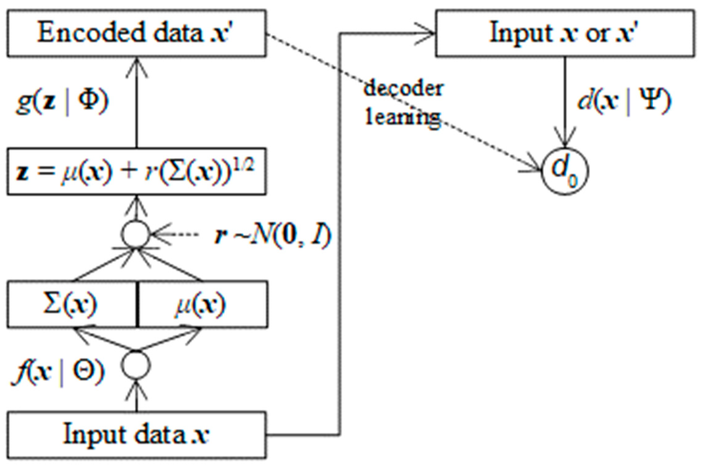
Figure 4.
AVA architecture with support of encoder assessing.
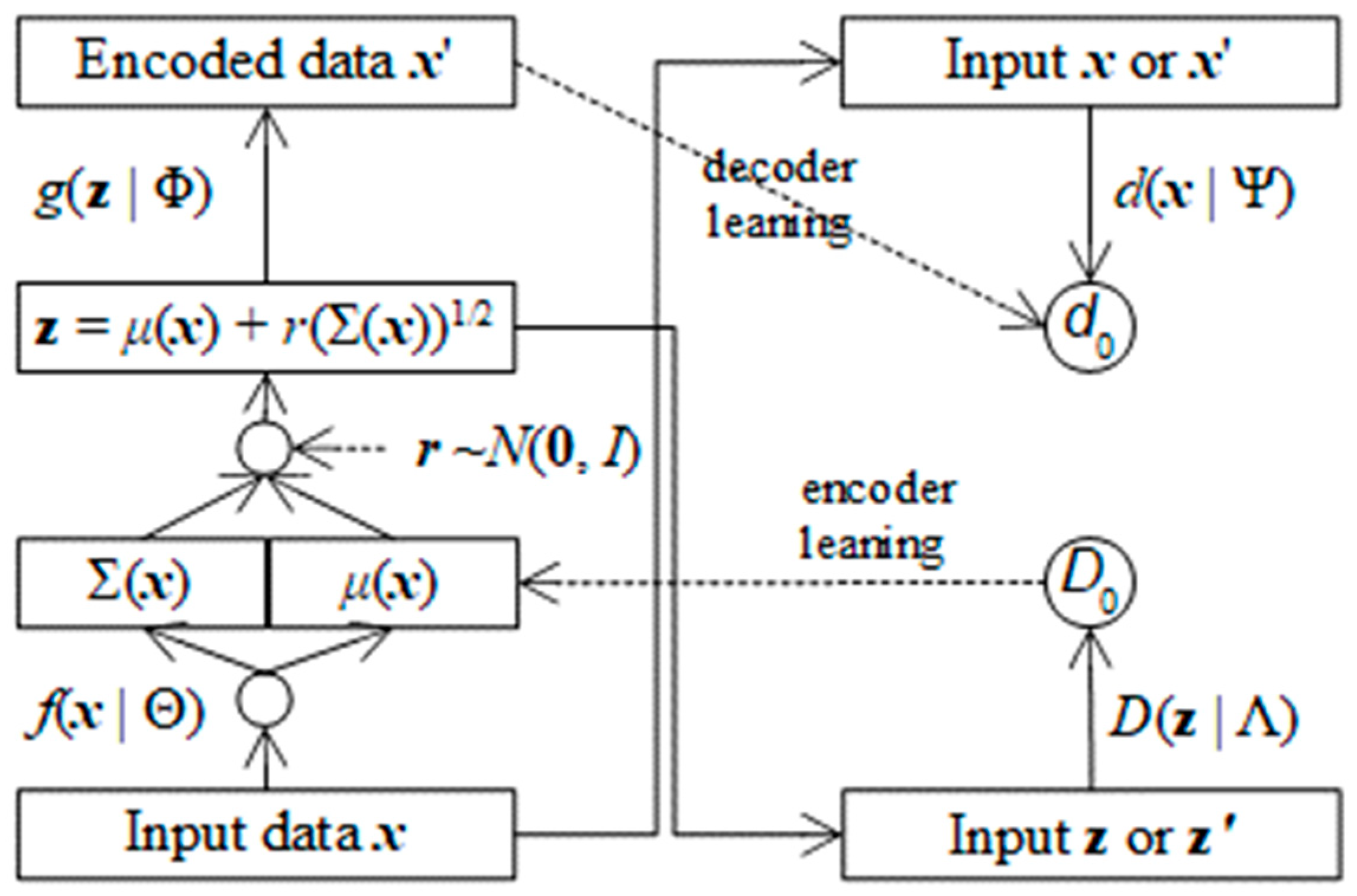
Figure 5.
Evaluation of AVAs and VAE.
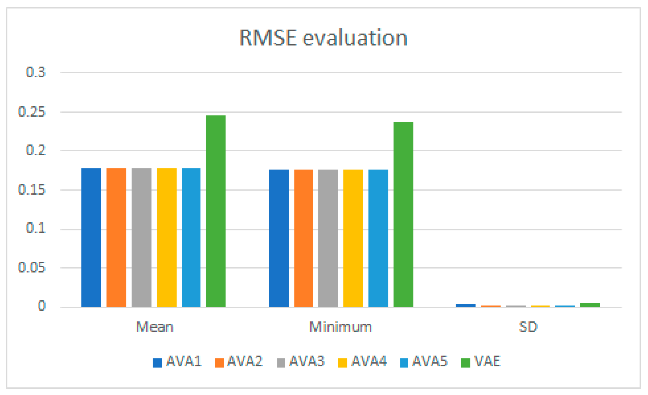

Table 1.
RMSE regarding learning rates from 1 down to 0.1.
| AVA1 | AVA2 | AVA3 | AVA4 | AVA5 | VAE | |
|---|---|---|---|---|---|---|
| γ=1 | 0.1776 | 0.1772 | 0.1772 | 0.1771 | 0.1777 | 0.2366 |
| γ=0.9 | 0.1775 | 0.1808 | 0.1773 | 0.1783 | 0.1806 | 0.2513 |
| γ=0.8 | 0.1887 | 0.1778 | 0.1777 | 0.1795 | 0.1778 | 0.2458 |
| γ=0.7 | 0.1793 | 0.1771 | 0.1834 | 0.1777 | 0.1797 | 0.2527 |
| γ=0.6 | 0.1774 | 0.1782 | 0.1770 | 0.1786 | 0.1774 | 0.2413 |
| γ=0.5 | 0.1774 | 0.1779 | 0.1775 | 0.1782 | 0.1811 | 0.2439 |
| γ=0.4 | 0.1772 | 0.1775 | 0.1776 | 0.1796 | 0.1778 | 0.2455 |
| γ=0.3 | 0.1769 | 0.1780 | 0.1796 | 0.1783 | 0.1775 | 0.2434 |
| γ=0.2 | 0.1777 | 0.1772 | 0.1769 | 0.1779 | 0.1776 | 0.2434 |
| γ=0.1 | 0.1778 | 0.1814 | 0.1765 | 0.1775 | 0.1775 | 0.2544 |
Table 2.
RMSE regarding learning rates from 0.09 down to 0.01.
| AVA1 | AVA2 | AVA3 | AVA4 | AVA5 | VAE | |
|---|---|---|---|---|---|---|
| γ=0.09 | 0.1773 | 0.1778 | 0.1784 | 0.1770 | 0.1774 | 0.2465 |
| γ=0.08 | 0.1783 | 0.1801 | 0.1835 | 0.1817 | 0.1777 | 0.2407 |
| γ=0.07 | 0.1831 | 0.1770 | 0.1775 | 0.1776 | 0.1802 | 0.2554 |
| γ=0.06 | 0.1782 | 0.1794 | 0.1784 | 0.1775 | 0.1786 | 0.2458 |
| γ=0.05 | 0.1786 | 0.1782 | 0.1789 | 0.1780 | 0.1774 | 0.2449 |
| γ=0.04 | 0.1774 | 0.1777 | 0.1775 | 0.1785 | 0.1768 | 0.2458 |
| γ=0.03 | 0.1799 | 0.1833 | 0.1774 | 0.1791 | 0.1776 | 0.2385 |
| γ=0.02 | 0.1777 | 0.1781 | 0.1775 | 0.1772 | 0.1792 | 0.2377 |
| γ=0.01 | 0.1776 | 0.1789 | 0.1784 | 0.1780 | 0.1787 | 0.2491 |
Table 3.
Evaluation of AVAs and VAE.
| AVA1 | AVA2 | AVA3 | AVA4 | AVA5 | VAE | |
|---|---|---|---|---|---|---|
| Mean | 0.1787 | 0.1786 | 0.1783 | 0.1783 | 0.1783 | 0.2454 |
| Minimum | 0.1769 | 0.1770 | 0.1765 | 0.1770 | 0.1768 | 0.2366 |
| SD | 0.0028 | 0.0017 | 0.0019 | 0.0011 | 0.0012 | 0.0054 |
Disclaimer/Publisher’s Note: The statements, opinions and data contained in all publications are solely those of the individual author(s) and contributor(s) and not of MDPI and/or the editor(s). MDPI and/or the editor(s) disclaim responsibility for any injury to people or property resulting from any ideas, methods, instructions or products referred to in the content. |
© 2023 by the authors. Licensee MDPI, Basel, Switzerland. This article is an open access article distributed under the terms and conditions of the Creative Commons Attribution (CC BY) license (http://creativecommons.org/licenses/by/4.0/).
Copyright: This open access article is published under a Creative Commons CC BY 4.0 license, which permit the free download, distribution, and reuse, provided that the author and preprint are cited in any reuse.


