Predictor-corrector Guidance for Hypersonic Morphing Vehicle

1. Introduction

Hypersonic morphing vehicle with a variety of sweep angles has stronger maneuverability [1]. The researches on this vehicle mainly focus on structure design [2], trajectory planning [3,4] and attitude control [5,6], among which trajectory planning method is a very important research content [3].

Trajectory planning of hypersonic vehicle is usually divided into reference trajectory method [7,8] and predictor-corrector method [9,10]. The predictor-corrector algorithm has strong online planning ability, and the method and its improvement are often used in the reentry guidance of hypersonic vehicle. Reference [11] using both the bank angle and attack angle as control variables, obtained much higher terminal altitude precision. Reference [12] proposed a novel quasi-equilibrium glide auto-adaptive guidance algorithm based on ideology of predictor-corrector, which meets the terminal position constraints. Reference [13] proposed a guidance law using extended Kalman filter to estimate the uncertain parameters in reentry flight of X-33, which is of great value to reconfigure the auto-adaptive predictor-corrector guidance. Reference [14] proposed a guidance algorithm based on the reference-trajectory and the predictor-corrector for the reentry vehicles, which has less computing time, high guidance precision, and good robustness. Reference [15] discussed recent developments in a robust predictor-corrector methodology for addressing the stochastic nature of guidance problems. Current predictor-corrector trajectory planning method for aircraft usually consists of three steps: 1) Determine the attack angle scheme, which usually is a linear transition mode. 2) Calculate the size of the bank angle according to the range error. 3) Calculate the bank angle sign according to the aircraft heading. For the hypersonic morphing vehicle in this paper, in order to improve the trajectory performance, it is necessary to design the sweep and angle scheme.

Reinforcement learning [16] and deep learning [17] methods have found many applications in trajectory planning algorithms due to their intelligence and high efficiency. In reference [18], a Back-Propagation neural network is trained by parameter profiles of optimized trajectory considering different dispersions to simulate the nonlinear mapping relationship between the current flight states and terminal states. The guidance method based on trajectory the neural network can well satisfy both path and terminal constraints and has good validity and robustness. Reference [19] presented a trajectory planning method based on Q-learning to solve the problem of HCV facing unknown threats. Reference [20] used reinforcement meta learning to optimize an adaptive guidance system suitable for the approach phase of a gliding hypersonic vehicle, which could induce trajectories that bring the vehicle to the target location with a high degree of accuracy at the designated terminal speed, while satisfying heating rate, load, and dynamic pressure constraints. Monte Carlo reinforcement learning [21] is a reinforcement learning used in controlling behavior [22]. This method is applied to many decision problems [23,24].

This article is divided into four parts:

• Establish the motion model of aircraft.
• The basic predictor-corrector algorithm is given. The Q-learning algorithm is used for attack and sweep angle scheme, which can cross the no-fly zones from above. B-spline curve method is used to solve the flight path points to ensure that the aircraft can cross the no-fly zones through the points. The size of bank angle is solved by the state error of the aircraft arriving at the target and flight point. The change logic of the bank angle sign is designed to ensure the aircraft flying safely to the target.
• The Monte Carlo Reinforcement Learning method is used to improve the predictor-corrector algorithm, and the Depth Neural Network is used to fit the reward function.
• Verify the effectiveness of the algorithm through simulation.

2. Materials and Methods

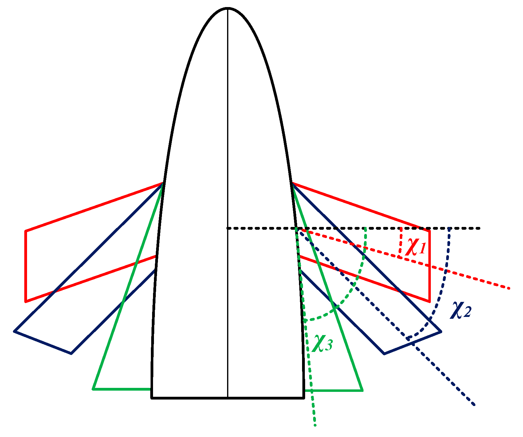
The shape of the aircraft is a wave-rider, with a top view as shown in Figure 1, and adopts bank-to-turn (BTT) control. The aircraft is composed of a body and foldable wings. The sweep angle of the wing can form three fixed sizes, respectively χ1=30°, χ2=45° and χ3=80°.

2.1. Aircraft Motion Model

According to reference [25], the equations of motion of the aircraft is established. Considering the following assumptions:

• The earth is a homogeneous sphere,
• The aircraft is a mass point which satisfies the assumption of instantaneous equilibrium,
• Sideslip angle β and the lateral force Z are both 0 during flight,
• Earth rotation is not taken into account.

The Equations of motion of the aircraft is given

$$\left\{\begin{array}{l}\frac{dr}{dt}=v\sin \theta \\ \frac{d\lambda }{dt}=\frac{v\cos \theta \sin \psi }{r\cos \varphi }\\ \frac{d\varphi }{dt}=\frac{v\cos \theta \cos \psi }{r}\\ \frac{dv}{dt}=-\frac{D}{m}-g\sin \theta \\ \frac{d\theta }{dt}=\frac{L\cos \sigma }{mv}+\left(\frac{v}{r}-\frac{g}{v}\right)\cos \theta \\ \frac{\mathrm{d}\psi }{\mathrm{d}t}=\frac{L\sin \sigma }{mv\cos \theta }+\frac{v}{r}\cos \theta \sin \psi \tan \varphi \end{array}\right.$$

(1)

where, t is the time, r denotes the distance between the aircraft's center of gravity, λ is longitude, ϕ is latitude, v is the aircraft speed, θ is the flight path angle, ψ is the heading angle, L is lift, and D is drag, α is the attack angle, σ is the bank angle, g is the acceleration of gravity. Define s as the flying range

$$\begin{array}{l}s=r_0{\beta }_c\\ {\beta }_c=\arcsin \frac{\sin \left(\lambda -{\lambda }_0\right)}{\sin \left(\arccos \left(\cos \left(\varphi -{\varphi }_0\right)\right)\cos \left(\lambda -{\lambda }_0\right)\right)}\end{array}$$

(2)

where, r₀=6371km is the Earth radius, (ϕ₀, λ₀) are the longitude and latitude of the starting point.

2.2. Constraint Model

• Heating rate constraint:

$${\dot{Q}}_s=k_Q\sqrt{\rho }{V}^{3.15}\le {\dot{Q}}_{s\max }$$

(3)

where, $\dot{Q}$ is the aircraft heating rate, in kW/m², and k_Q is the heating rate constant, ${\dot{Q}}_{s\max }$ is the maximum allowable heating rate.

2.

Dynamic pressure q constraint:

$$q=0.5\rho V^2\le q_{\max }$$

(4)

where, q_max is the maximum allowable dynamic pressure, in Pa.

3.

Overload n constraint:

$$n=L\cos \alpha +D\sin \alpha \le n_{\max }$$

(5)

where, n_max is the maximum allowable dynamic pressure. The aircraft in this paper has three sizes of sweep angle, corresponding to three kinds of available overloads.

4.

No-fly Zone Model

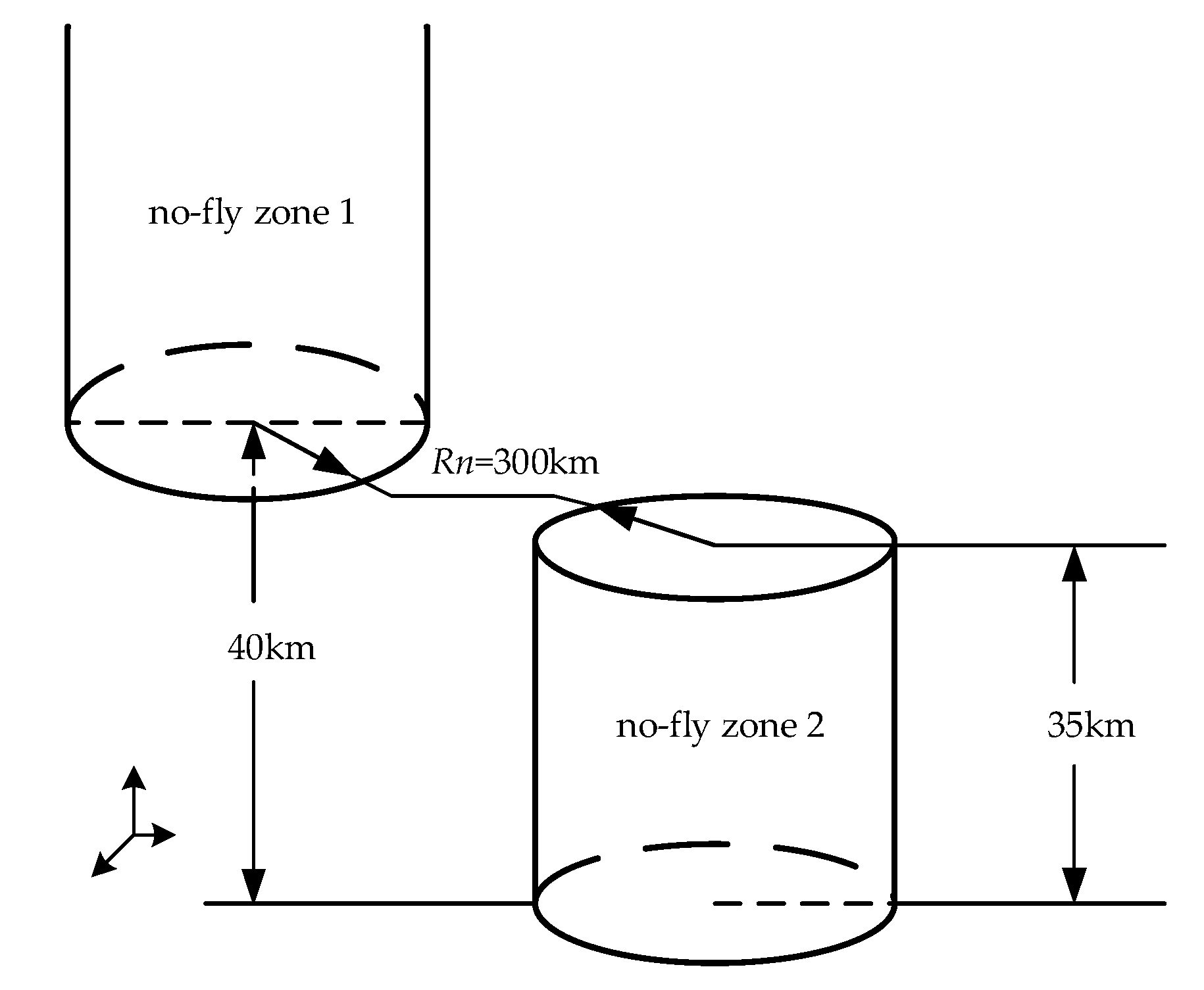
In this paper, two types of no-fly zone are considered. type 1 is high-altitude no-fly zone, whose model is a cylinder with a base surface of h = 40km and a radius of R_n = 300km. type 2 is low-altitude no-fly zone, whose model is a cylinder with a base surface on the ground and a top surface 35km high and a radius of 300km. The two types no-fly zones are shown in Figure 2. The model of the no-fly zone is given as

$$\begin{array}{l}{r}^2{\sin }^2\Delta \beta \ge R_n^2\\ \left\{\begin{array}{l}h>35km\\ h<40km\end{array}\right.\end{array}$$

(6)

where, Δβ= arccos(sinϕnsinϕ+cosϕ_ncosϕcos(λ-λ_n)), (λ_n, ϕ_n) is the center of the no-fly zone.

3. Basic Predictor-corrector Guidance Algorithm

This section introduces the basic predictor-corrector guidance algorithm, which can achieve the function of the aircraft to avoid no-fly zones during flight and reach the target point. The results of the basic algorithm will be input into the improved algorithm learning network as a sample, providing training and evaluation data. The basic algorithm includes attack angle and sweep angle scheme, flight path point plan, and bank angle scheme.

3.1. Attack Angle and Sweep Angle Scheme

In this section, the Q-learning algorithm is used to give the attack angle and sweep angle scheme to avoid type 2 no-fly zones.

3.1.1. Q-learning Principles

In the Q-learning algorithm, firstly, calculate the immediate reward r_t=R(s_t,a_t) after state s_t performing the action at. Then calculate the state-action value function discount value γmaxQ(s_t+1, a) for the next state st+1. Then the value function Q(s_t,a_t) in current state can be estimated. If there are m states and n actions, the Q-table is a m×n matrix.

The algorithm is to find the optimal strategy π* by estimating the value of the state-action value function Q(s_t,a_t) in each state. The rows of the Q- table represent the states in the environment, and the columns of the table represent the actions that the aircraft can perform in state. In the process of trajectory planning, the environment will provide feedback to the aircraft through reinforcement signals (reward function). During the learning process, the Q-value of the actions that are conducive to completing the task becomes larger as the number of times they are selected, while those are not conducive to task completion will become smaller. Through multiple iterations, the action selection strategy π of the aircraft will converge to the optimal action selection strategy π*.

The rule for updating Q-values is

$$Q\left(s_t,a_t\right)=r_t+\gamma \underset{a\in A}{\max }Q\left(s_{t+1},a\right)$$

(7)

where, maxQ(s_t+1, a) is the Q-value corresponding to action a with the biggest Q-value found in action set A when the aircraft is in state s_t+1. The iterative process of Q-value can be obtained as follows

$$Q_{k+1}\left(s_t,a_t\right)\leftarrow Q_k\left(s_t,a_t\right)+\left(r_t+\gamma \underset{a\in A}{\max }{Q}_{k+1}\left(s_{t+1},a\right)-Q_k\left(s_t,a_t\right)\right)$$

(8)

where, k is the k-th iteration, α∈(0,1) is learning efficiency and controls the speed of learning. The larger its value, the faster the algorithm converges. Generally, it takes a constant.

Q-learning approximates the optimal state action value function Q*(s, a) by updating the strategy. Q*(s, a) is the maximum Q-value function among all policies π, represented by

$$Q^{*}\left(s,a\right)=\underset{\pi }{\max }{Q}_{\pi }\left(s_t,a_t\right)$$

(9)

where, Q(s_t,a_t) is the state-action value function of all strategies π, and Q*(s, a) is the maximum value function, corresponding to the optimal strategy π*. According to the Bellman optimal equation, there is

$$Q^{*}\left(s,a\right)={\displaystyle \sum _{s\in S}\left[R_s^a+\gamma {\max }_{a_{t+1}}{Q}^{*}\left(s_{t+1},a\right)\right]}$$

(10)

where, $R_s^a$ represents the immediate reward obtained by executing action at in state s_t and reaching state s_t+1. This paper adopts greedy strategy.

The basic process of Q-learning algorithm is as follows:

• Selection algorithm parameters: α∈(0,1), γ∈(0,1), maximum iteration steps t_max.
• Initialization: For all s∈S, a∈A (s), initialize Q(s, a)=0, t=0.
• For each learning round:

Initialize state s_t.

Using the strategy π, randomly select a_t at s_t, update Q:

$$Q\left(S_t,A_t\right)\leftarrow Q_k\left(S_t,A_t\right)+\alpha \left[R+\gamma \underset{A}{\max }Q\left(S_{t+1},A\right)-Q\left(S_t,A_t\right)\right]$$

(11)

4.

Reach the termination state, or t>t_max.

3.1.2. Q-learning Algorithm Setting

The Q-learning network takes the aircraft motion model and the environment as inputs to obtain attack and sweep angle scheme. The parameters are set as follows.

• State set

The state in the algorithm needs to be determined based on the flight process. Considering that the range during the flight process usually vary monotonically, using it as state variable can make the state variables exhibit a one-dimensional trend, which can avoid random changes between state variables, and reduce the dimension of state variables to simplify the algorithm. The initial expected range of the aircraft is 6000km, with every 300km as a state, there can be 20 states: S (S₁, S₂, ..., S₂₀) = {0km, 300km, ..., 6000km}. At this time, there is no need to set a state transition function, and the state transition is Si → S_i+1 (i=1... 19).

2.

Action set

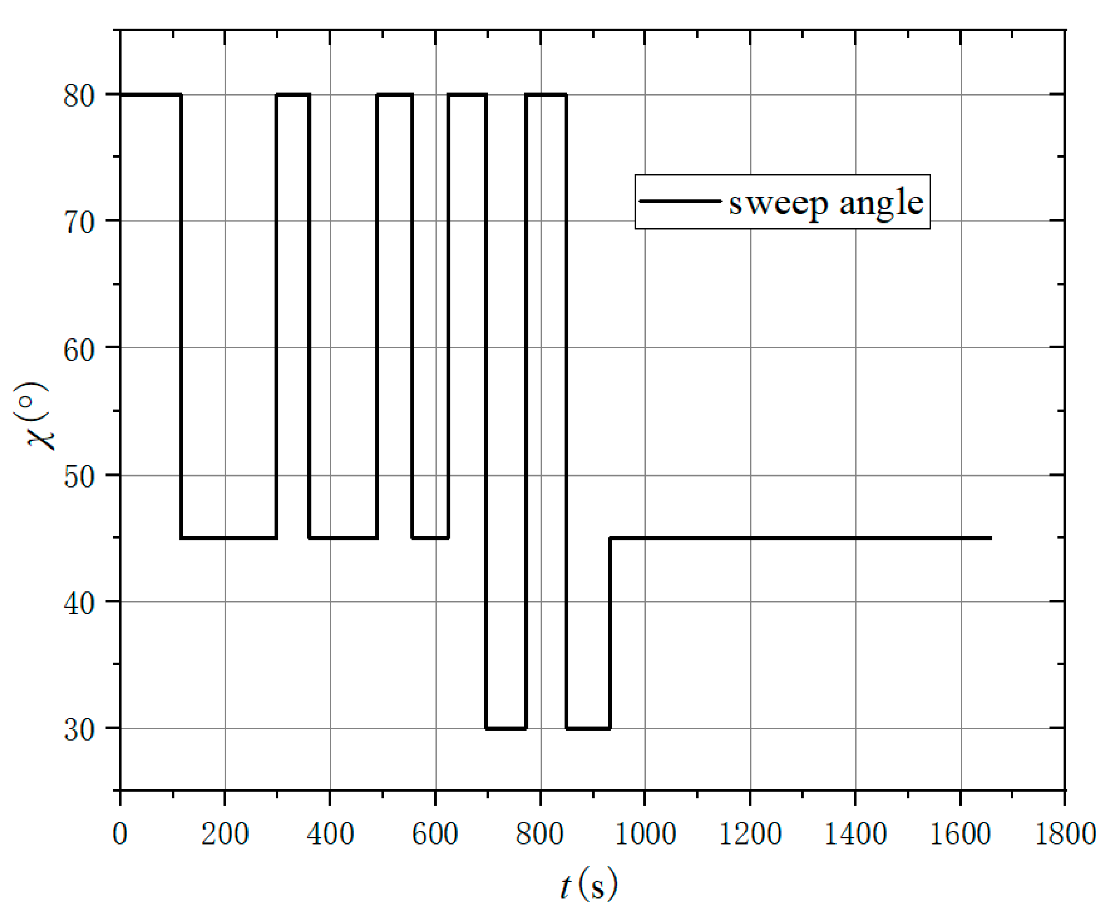
Set action set A_i = (χ, α), which includes the sweep angle and attack angle. The sweep angle includes 30°, 45°, and 80°, the range of angle of attack values is 5°~25°. Taking 5° is the interval, five conditions can be taken as 5°, 10°, 15°, 20°, and 25° respectively, to obtain 15 actions. The action set can be expressed as A = {A₁(30°, 5°), A₂(30°, 10°), ..., A₁₅(80°, 25°)}.

3.

Reward function

The setting of the reward function is crucial as it relates to whether the aircraft can avoid no-fly zones and reach the target. The rationality of it directly affects the learning efficiency. Based on the environment, reward function is set as follows

$$R(s,a)=\left\{\begin{array}{l}{R}_b\hspace{0.33em}\hspace{0.33em}\hspace{0.33em}\hspace{0.33em}\hspace{0.33em}\hspace{0.33em}\hspace{0.33em}\hspace{0.33em}\hspace{0.33em}\hspace{0.33em}\hspace{0.33em}\hspace{0.33em}s\in S_{\mathrm{no}-\mathrm{fly}\mathrm{zone}}\\ R_f=e/e_0\hspace{0.33em}\hspace{0.33em}\hspace{0.33em}\hspace{0.33em}\hspace{0.33em}\hspace{0.33em}\hspace{0.33em}\hspace{0.33em}s\in S_{\mathrm{normal}}\\ R_t\hspace{0.33em}\hspace{0.33em}\hspace{0.33em}\hspace{0.33em}\hspace{0.33em}\hspace{0.33em}\hspace{0.33em}\hspace{0.33em}\hspace{0.33em}\hspace{0.33em}\hspace{0.33em}\hspace{0.33em}\hspace{0.33em}\hspace{0.33em}s\in S_{\mathrm{target}}\\ R_{c\hspace{0.33em}\hspace{0.33em}\hspace{0.33em}\hspace{0.33em}\hspace{0.33em}\hspace{0.33em}\hspace{0.33em}\hspace{0.33em}\hspace{0.33em}\hspace{0.33em}\hspace{0.33em}\hspace{0.33em}\hspace{0.33em}\hspace{0.33em}\hspace{0.33em}\hspace{0.33em}\hspace{0.33em}\hspace{0.33em}\hspace{0.33em}\hspace{0.33em}\hspace{0.33em}\hspace{0.33em}\hspace{0.33em}\hspace{0.33em}\hspace{0.33em}\hspace{0.33em}\hspace{0.33em}}s\in S_{\mathrm{prograss}\mathrm{constraint}}\end{array}\right.$$

(12)

where, R_b and R_n are the rewards obtained by the aircraft when entering the no-fly zone and normal flight respectively, where Rb is set as a constant less than 0 to guide the aircraft to avoid the no-fly zone, and R_f is set as a reward related to the aircraft velocity to enable the aircraft to store more velocity when reaching the target, R_t is the reward for the arrival to the target, and setting it as a constant greater than 0 can guide the aircraft to reach the desired range, R_c is the reward when the aircraft does not meet flight constraints, set to a constant less than 0 to ensure the safety of the aircraft's flight performance.

In this section, the avoidance of type 2 no-fly zone has been achieved through attack and sweep angle scheme, while type 1 zone needs to be avoided through lateral flight. The following is the lateral trajectory scheme. The attack and sweep angle schemes obtained in this section will be provided as inputs to the lateral planning algorithm.

3.2. Flight Path Point Plan

For the no-fly zones present in the environment, it is necessary to design avoidance methods. In the analysis in last section, it can be seen that the type 2 zone can be avoided by pulling up the trajectory, while the type 1 can’t. Therefore, type 1 zone needs to be avoided through lateral maneuvering, and it is necessary to plan the lateral trajectory. The B-spline curve is used to obtain flight path points, and the lateral guidance of the aircraft is realized by tracking the points.

3.2.1. B-spline curve principle

B-spline curve is composed of starting point, ending point, and control points. By adjusting the control points, the shape of the B-spline curve can be changed. B-spline curves are widely used in various trajectory planning problems due to its controllable characteristics [26]. The B-spline curve is expressed as

$$B\left(\tau \right)={\displaystyle \sum _{i=0}^n{C}_n^i{P}_i{\left(1-\tau \right)}^{n-i}{\tau }^i,\tau \in \left[0,1\right]}$$

(13)

where, P_i is the control point of the curve, P₀ is the starting point, P_n is the end point, n is the order of curve. As long as the first and last control points of two B-spline curves are connected and the four control points at the connection are collinear, it can be ensured that the curve has the same position at the connection and the first derivative of the curve is the same. The concatenated curve will still be a B-spline curve. The lateral trajectory planning of aircraft can be realized by using this property.

3.2.2. No-fly Zone Avoidance Methods

Considering the horizontal environment model, the no-fly zone is projected from a cylinder in a circle. Design a 2-D B-spline curve that satisfies the constraint, and then flight path points are obtained according to curve control points. The planning method is divided into the following steps:

• Based on the location of the circles, choose an appropriate direction to get the tangent points of the circles, and then select different combinations of tangent points to obtain the initial control points. If the initial point and target line through the threat zone, at least one tangent point is selected as the control point, and at most one tangent point is selected for each zone.
• Augment initial control point set. The initial augmentation control point is located on the initial heading to ensure the initial heading angle, and the intermediate augmented control points are located on both sides of the tangent points, then the control point set is obtained. The initial position P₀ and end position P_n of the curve correspond to the initial position of the aircraft and the target. In order to ensure that the aircraft can avoid the threat area, as long as the aircraft is on the other side of the threat area tangent line Therefore, the B-spline curve is designed to be tangent to the circle of the zone. According to the characteristic of the curve, the tangent point can be the middle point of three collinear control points. Then adjust the distance d₁ and d₂ between the two adjacent control points to control the curvature of the curve near the tangent point so that it does not intersect the circle, as shown in Figure 3. In the figure, P₀~P₄ are control points, and the red spline curve is tangent to the no-fly zone, avoiding the curve from crossing the zone.

Choose the tangent point (P₂) of the circle as the initial control point, and augment two control points (P₁, P₃) on both sides of the tangent point. The augmented control points are given by the distance (d₁, d₂) from the tangent point.

3.

Take the distance between the tangent point and the augmented point as the optimization variable. Take the spline curve length and mean curvature as the performance indicators. The optimal curve is obtained through genetic algorithm, and the control points are obtained. The optimization model is as follows:

$$\begin{array}{l}P：\min J_1=f_1\left(d_{1,}\mathrm{...}{d}_n\right)=L_b\\ \hspace{0.33em}\hspace{0.33em}\hspace{0.33em}\hspace{0.33em}\hspace{0.33em}\hspace{0.33em}{J}_2=f_2\left(d_{1,}\mathrm{...}{d}_n\right)=n_b\\ s.t.\hspace{0.33em}{P}_0=\left({\lambda }_0,{\varphi }_0\right)\\ \hspace{0.33em}\hspace{0.33em}\hspace{0.33em}\hspace{0.33em}\hspace{0.33em}{P}_n=\left({\lambda }_t,{\varphi }_t\right)\end{array}$$

(14)

where, J₁ and J₂ are two performance index functions, L_b is the equivalent length of the curve, and n_b represents the mean curvature of the curve. The equations are as follows

$$\begin{array}{l}{L}_b={\displaystyle \underset{0}{\overset{1}{\int }}\sqrt{{\left({{\lambda }^{\prime }}_{\tau }\right)}^2+{\left({{\varphi }^{\prime }}_{\tau }\right)}^2}}d\tau \\ n_b=\frac{{{\lambda }^{\prime }}_{\tau }{{\varphi }^{″}}_{\tau }-{{\lambda }^{″}}_{\tau }{{\varphi }^{\prime }}_{\tau }}{{\left({\left({\lambda }_{\tau }\right)}^2+{\left({\varphi }_{\tau }\right)}^2\right)}^{3/2}}\end{array}$$

(1)

It should be noted that the curve is not the lateral trajectory of the aircraft, so its length cannot represent the flight range, and its curvature cannot represent the overload of the aircraft. However, as characteristics of the curve, they can be used to evaluate the performance of the curve. Obtain the optimal B-spline curves through optimization. Discard the curve that crosses the no-fly zones, and then select the one with the best performance index from all curves.

4.

Simplify the control points to obtain the flight path points.

The simplification rules are as follows: 1) Simplify from the beginning point to the end point, and delete the augmented control point of the starting point. 2) If multiple points are located on one line segment, delete the intermediate points and leave the two endpoints. 3) If there are four consecutive control points (P0~P3), after deleting the second control point P1, the angle of connecting lines by P0-P2-P3 is bigger than the original and does not cross the no-fly zone, delete the second control point P1.4) When the simplification is repeated until two consecutive point set are identical, the simplify finish.

3.3. Bank Angle Scheme

Bank angle scheme includes size and sign scheme.

3.3.1. Bank Angle Size Scheme

Bank angle size scheme is achieved through predictor-corrector algorithm. First, the horizontal error of the flight path point is predicted based attack and sweep angle scheme, and then the amplitude and size of the bank angle are corrected.

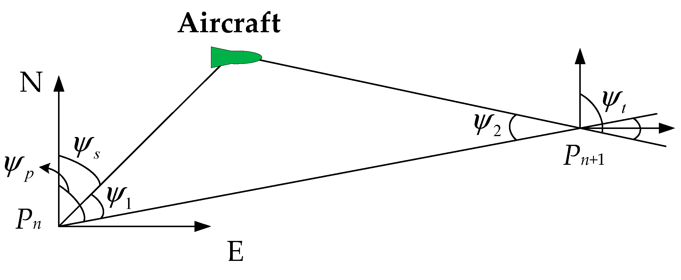
Based on the attack angle, sweep angle, the initial bank angle, integrating the equation of motion until the vehicle reaches the next path point. Then, the latitude position error e_ϕ and the velocity error e_v are obtained. Using the secant method, the amplitude of the bank angle |σ_max| is corrected by e_v. and the size of the bank angle |σ| is corrected by e_ϕ. When the aircraft is between two points P_n and P_n+1, there is a relationship as shown in Figure 4.

The correction process for the size of bank angle is given as follows.

(1) Taking initial σ₀₌20°, integrate the equations of motion to the longitude of the target, and calculate the e_v.

(2) For intermediate path points, if e_v is less than 10% of the expected speed, correction is completed. otherwise σ₀= σ₀+sgn(e_v), return to step (1). For the trajectory endpoint, no correction is required, and take σ₀= σ₀+1.

To avoid big overshoot of position when the aircraft passing through the path point line, The bank angle size is set to be related to ψ₁ and ψ₂ in Figure 4. This will reduce the bank angle as the aircraft approaches the path point connection line, the scheme is as follows

$$\left\{\begin{array}{l}\left|\sigma \right|=k_e{\psi }_1\le \left|{\sigma }_{\max }\right|\hspace{0.33em}\hspace{0.33em}\hspace{0.33em}\hspace{0.33em}\hspace{0.33em}{\psi }_1\ge {\psi }_2\\ \left|\sigma \right|=k_e{\psi }_2\hspace{0.33em}\le \left|{\sigma }_{\max }\right|\hspace{0.33em}\hspace{0.33em}\hspace{0.33em}\hspace{0.33em}{\psi }_2>{\psi }_2\end{array}\right.$$

(16)

where, k_e>0 is the coefficient of bank angle error, which is determined by e_φ. The correction process is as follows.

(1) Taking initial σ₀ satisfied |σ₀|<|σ_max|, get k_e1 at this time, integrate the motion equations to the longitude of target, and get the e_ϕ1.

(2) Taking σ₀=0, and k_e0=0 at this time, integrate the equations of motion to the longitude of next path point, and calculate e_ϕ0.

(3) k_e is obtained by the correction equation

$$k_e=k_{e1}-e_{\varphi 1}\frac{e_{\varphi 1}-e_{\varphi 0}}{k_{e1}-k_{e0}}$$

(17)

(4) Integrate the motion equations to the longitude of target, and then calculate e_ϕ.

(5) If e_ϕ < 0.01, correction progress is completed, otherwise, e_ϕ1= min(e_ϕ1, e_ϕ0). Update k_e1, and take k_e0= k_e, e_ϕ0=e_ϕ, return to step (3).

The above is the scheme of bank angle size.

3.3.2. Bank Angle Sign Scheme

After obtaining the set of flight path points, each point should be tracked to ensure the correct heading of the aircraft. At this time, it is necessary to give the change rule of the bank angle sign.

Heading angle ψ_Los of the connecting line at point (λ₁, ϕ₁) and (λ₂, ϕ₂) is

$${\psi }_{Los}=\arctan \frac{\sin \left({\lambda }_1-{\lambda }_2\right)}{\cos {\varphi }_1\tan {\varphi }_1-\sin {\varphi }_1\cos \left({\lambda }_1-{\lambda }_2\right)}$$

(18)

ψ₁= ψ_s-ψ_p and ψ₂= ψ_t-ψ_p are the heading angle of the aircraft and the connecting line between the front and back path points. It is known that ψ₁ and ψ₂ have different sign. If the aircraft is located on the left side of the path point line (as shown in Figure 4), then ψ₁<0 and ψ₂>0. The aircraft needs to adjust the heading angle to increase, and the bank angle is a positive sign. If the aircraft is located on the right side of the waypoint line (as shown on the other side), then ψ₁>0 and ψ₂<0, the aircraft needs to adjust its heading angle to reduce, and the bank angle is a negative sign. The bank angle sign changing logic is

$$\mathrm{sgn}\left(\sigma \right)=-\mathrm{sgn}\left({\psi }_1\right)=\mathrm{sgn}\left({\psi }_2\right)$$

(19)

where, sgn(·) is a sign function.

The above is the entire process of the basic predictor-corrector guidance algorithm.

4. Improving Predictor-corrector methods

In this paper, the MCRL method [27] is used to improve the basic predictor-corrector algorithm. The Monte Carlo Reinforcement learning algorithm is used to improve the predictor-corrector algorithm, and the basic algorithm is used to obtain the sample for training MCRL net. According to the reward calculated by the errors of aircraft state reaching path points, the optimal control command is trained. The reward function solution is fitted by the DNN to improve the efficiency of the algorithm.

4.1. Monte Carlo Reinforcement Learning Method

In MCRL method, the learning sample is obtained by a large number of calculations of the model, and the average reward is taken as the approximate value of the expected reward. The method directly estimates the behavior value function, in order to get the optimal behavior directly by ε-greedy strategy.

4.1.1. MCRL Principle

The behavior value function Q is

$$\begin{array}{ll}{Q}_{\pi }\left(s,a\right)& =E_{\pi }\left[G_t|S_t=s,A_t=a\right]\\ & =E_{\pi }\left[R_{t+1}+\gamma R_{t+2}+\cdots |S_t=s,A_t=a\right]\\ & =E_{\pi }\left[{\displaystyle \sum _{k=0}^{\infty }{\gamma }^k{R}_{t+k+1}|}{S}_t=s,A_t=a\right]\end{array}$$

(20)

where R is the reward of one step.

For model-free MCRL method, information needs to be extracted from samples and the average reward of each state s_t is calculated as the expected reward. It is necessary to use strategy π to generate multiple complete trajectories from the initial state to the termination state, and calculate the reward value of each trajectory. The solution equation is as follows

$$\begin{array}{l}{G}_t=R_{t+1}+\gamma R_{t+2}+\cdots ={\displaystyle \sum _{k=0}^{\infty }{\gamma }^k{R}_{t+k+1}}\\ Q\left(s\right)=\frac{a_1{G}_1+a_2{G}_2+\cdots }{N\left(s,a\right)}\end{array}$$

(21)

where, a₁, a₂, ... are discount coefficients, a₁+a₂+...=1.

The algorithm adopts ε-greedy strategy for action selection. The strategy randomly selects an action from action set with a probability of ε and changes it to 1-ε. Assuming that there are n actions, the probability that the optimal action is selected is 1-ε+ε/n, and the equation of the ε-greedy algorithm is

$$\pi \left(s|a\right)=\left\{\begin{array}{l}\frac{\epsilon }{n}+1-\epsilon \hspace{1em}\hspace{1em}a*=\arg \underset{a\in A}{\max Q\left(s,a\right)}\\ \frac{\epsilon }{n}\hspace{1em}\hspace{1em}\hspace{1em}\mathit{others}\end{array}\right.$$

(22)

Under this strategy, the probability of selecting each action in the action set is non-zero, which increases the probability of selecting the optimal action while ensuring sufficient exploration action.

In this paper, the importance sampling method is used to evaluate strategy π with strategy π’. When the ε-greedy strategy is adopted to evaluate the greedy strategy, the equation for updating the action value function is

$$Q\left(s_t,a_t\right)\leftarrow Q\left(s_t,a_t\right)+\alpha \left({\displaystyle \prod _{i=t}^{T-1}\frac{1}{p_i}G}-Q\left(s_t,a_t\right)\right)$$

(23)

The MCRL algorithm is as follows.

Algorithm: MCRL algorithm   Input: environment E, state space S, action space A, initialization behavior value function Q.   Output: Optimal strategy π *.   Initialize Q(s, a) = 0, total reward G=0   For k=0, 1, ..., n   Execute in E ε-greedy strategy π'generates trajectory   $p_i=\left\{\begin{array}{l}1-\epsilon +\frac{\epsilon }{m}{a}_i=\pi \left(s_i\right)\\ \frac{\epsilon }{m}{a}_i\ne \pi \left(s_i\right)\end{array}\right.$   For t=0, 1, 2, ..., n      $\forall s_t\in S\forall a_t\in A$      $G={\displaystyle \sum _{i=t}^T{\gamma }^{i-t}{r}_i}$      $Q\left(s_t,a_t\right)\leftarrow Q\left(s_t,a_t\right)+\alpha \left({\displaystyle \prod _{i=t}^{T-1}\frac{1}{p_i}G}-Q\left(s_t,a_t\right)\right)$     End for $\forall s_t\in S^{\prime }:\pi \left(s_t\right)=\arg \underset{a\in A}{\max }Q\left(s_t,a_t\right)$ End for

4.1.2. MCRL Method Settings

The MCRL method includes state sets, action sets, and reward functions. The parameters are set as follows.

(1) State set

There are two waypoints on the flight trajectory, which can be divided into three sections: starting point→path point 1→path point 2→endpoint. In the MCRL method, algorithm state is the flight state set S_fly = (h, λ, ϕ, v, θ, ψ). At this point, the state set consists of three states, which are S(S₁, S₂, S₃) = {starting point, path point 1, path point 2}. There is no need to set a state transition function, and the state transition is S_i→S_i+1(i= 1,2,3).

(2) Action set

Design the action A_i= (|σ_max|_i, k_ei), including the amplitude and error coefficient of the bank angle. The value of the bank angle amplitude ranges from 0° to 30°, with 31 groups at an interval of 1°. The error coefficient of bank angle has different ranges in different trajectory sections. The coefficients k_e1 and k_e2 range from 0 to 20, with 21 groups at an interval of 1, and k_e3 ranges from -0.3 to 0.1 with 41 groups at an interval of 0.01. The action set A= {A₁, A₂, A₃} is got.

(3) Reward function

The reward function considers three states when the aircraft reaches the target: the latitude error e_ϕ, the speed v_t and the heading angle error e_ψ = ψ-ψ_Los. The equation of reward function is

$$\left\{\begin{array}{l}0\hspace{1em}\hspace{1em}{e}_{\varphi }>e_{\varphi \max }\\ b_1{e}^{-\frac{{\left(v_t-\mu \right)}^2}{{\sigma }_1^2}}+b_2{e}^{-\frac{e_{\psi }^2}{{\sigma }_2^2}}+b_3-b_3{e}^{-\frac{e_{\varphi }^2}{{\sigma }_2^2}}\hspace{1em}\hspace{1em}{e}_{\varphi }\le e_{\varphi \max }\end{array}\right.$$

(24)

where, μ is the offset coefficient, σ₁, σ₂ and σ₃ is the scaling coefficient, b₁, b₂ and b₃ are the weight coefficients, and b₁+b₂+b₃=1. When the error e_ϕ does not meet the error boundary, it is considered that the aircraft cannot reach the expected position, and the reward is 0. When the error meets the error boundary, the reward is obtained from the above three items.

4.2. Deep Neural Network Fitting the Reward Function

• DNN principle

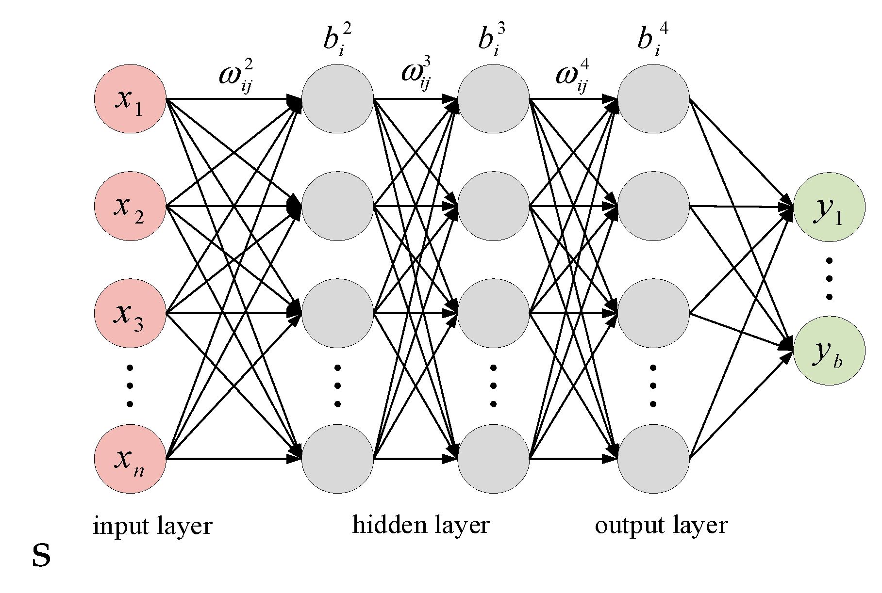
This article uses a DNN net to fit the reward function. The basic structure of DNN is shown in Figure 5, which can be divided into input layer, hidden layer, and output layer. In the figure, ω is the weight coefficient, b is the threshold, with a superscript representing the number of layers, and a subscript representing the number of neurons. Assuming that the activation function is f(), the number of neurons in the first hidden layer is m, and the output is a, then the output of layer l is

$${\mathrm{a}}^l=f\left(z^l\right)=f\left({\mathrm{W}}^l{\mathrm{a}}^{l-1}+{\mathrm{b}}^l\right)s$$

(25)

2.

DNN settings

The network consists of three hidden layers with 10 neurons in each hidden layer. The network structure is "n_input-10-10-10-n_output", where, "n_input" and "n_output" are the quantities of input and output determined by the sample. Then map the sample data in [−1, 1] by normalization equation

$$\overline{x}=\frac{x-x_{\min }}{x_{\max }-x_{\min }}+\frac{x-x_{\max }}{x_{\max }-x_{\min }}$$

(26)

In this paper, feedforward backpropagation network, backpropagation training function, gradient descent learning function, average data performance variance and tansig transfer function are selected. The tansig function equation is

$$\tan \mathrm{sig}(x)=\frac{2}{1+e^{-2x}}-1$$

(27)

It takes four passes from the input layer to the output layer. After the learning, four weight matrices (W₁, W₂, W₃, W₄) and four threshold matrices (b₁, b₂, b₃, b₄) will be obtained. For input x, network output y

$$y=W_4\tan \mathrm{sig}\left(W_3\tan \mathrm{sig}\left(W_2\tan \mathrm{sig}\left(W_{1}x+b_1\right)+b_2\right)+b_3\right)+b_4$$

(28)

5. Simulation

The initial altitude of the aircraft is h₀ = 68km, the longitude and latitude are (λ₀ = 0°, ϕ₀ = 0°), the velocity is v₀ = 5300m/s, the initial ballistic inclination Angle of the aircraft, the attack angle α₀ and the bank angle σ₀ are all 0°, the initial heading angle ψ₀ = 85°, and the target point is located at (λ_t = 53.8°. ϕ_t = 5.4°), the expected range s = 6000km. There are two type 1 no-fly zones, with the center located at (23°, 4.5°) and (37°, 1.5°), and two type 2 no-fly zones, with the center located at (30°, 3°) and (45°, 6°).

5.1. Simulation of Attack and Sweep Angle Scheme

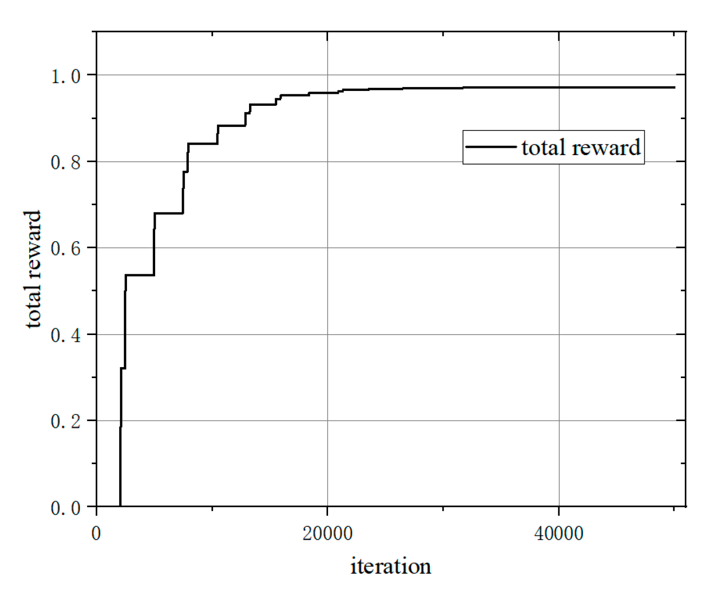
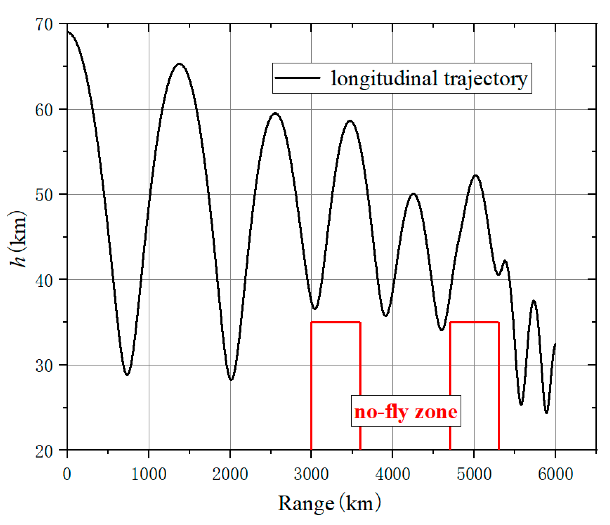
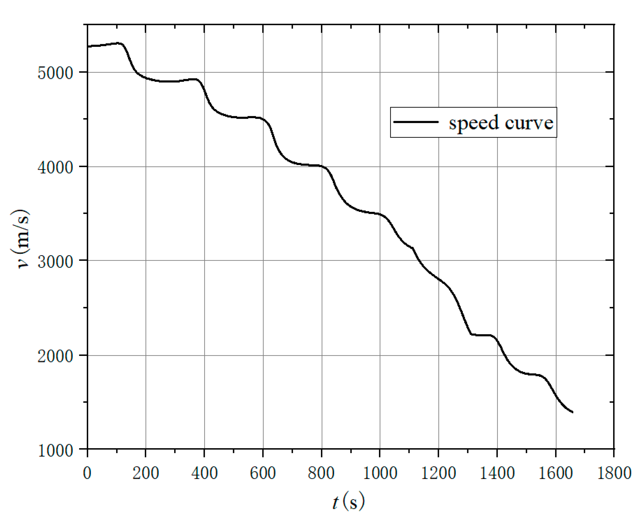
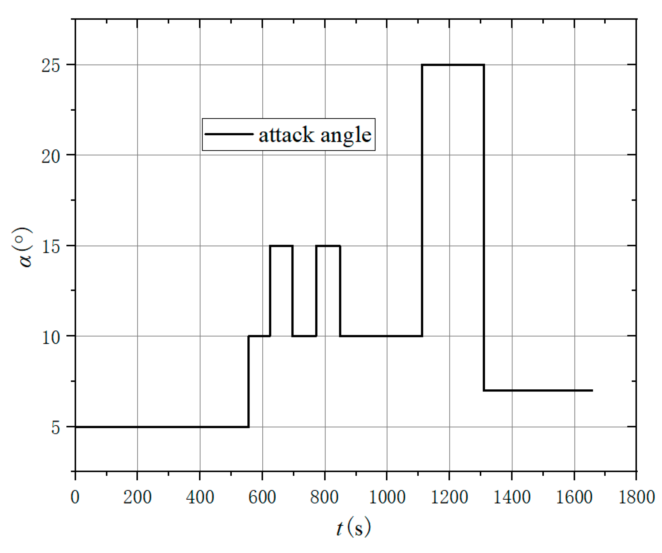
According to the environment, two type 2 zones are set up, and take σ = 20°. After 50000 studies, the total reward and flight process status are shown as follows.

Figure 6. Total Reward Curve.

Figure 6. Total Reward Curve.

Figure 7. Longitudinal trajectory.

Figure 7. Longitudinal trajectory.

Figure 8. Speed curve.

Figure 8. Speed curve.

Figure 9. Attack angle curve.

Figure 9. Attack angle curve.

Figure 10. Sweep angle curve.

Figure 10. Sweep angle curve.

Based on the above results, the trajectory could avoid type 2 no-fly zones, and the total reward of the algorithm tends to converge after 30000 learning. The longitudinal trajectory of the aircraft can avoid the zones and fly to a range of 6000km. The aircraft uses both the attack angle and the sweep angle to pull up the trajectory in front of the zone, causing the trajectory to fly higher and maintain height over 35km.

5.2. Flight Path Point Planning Results

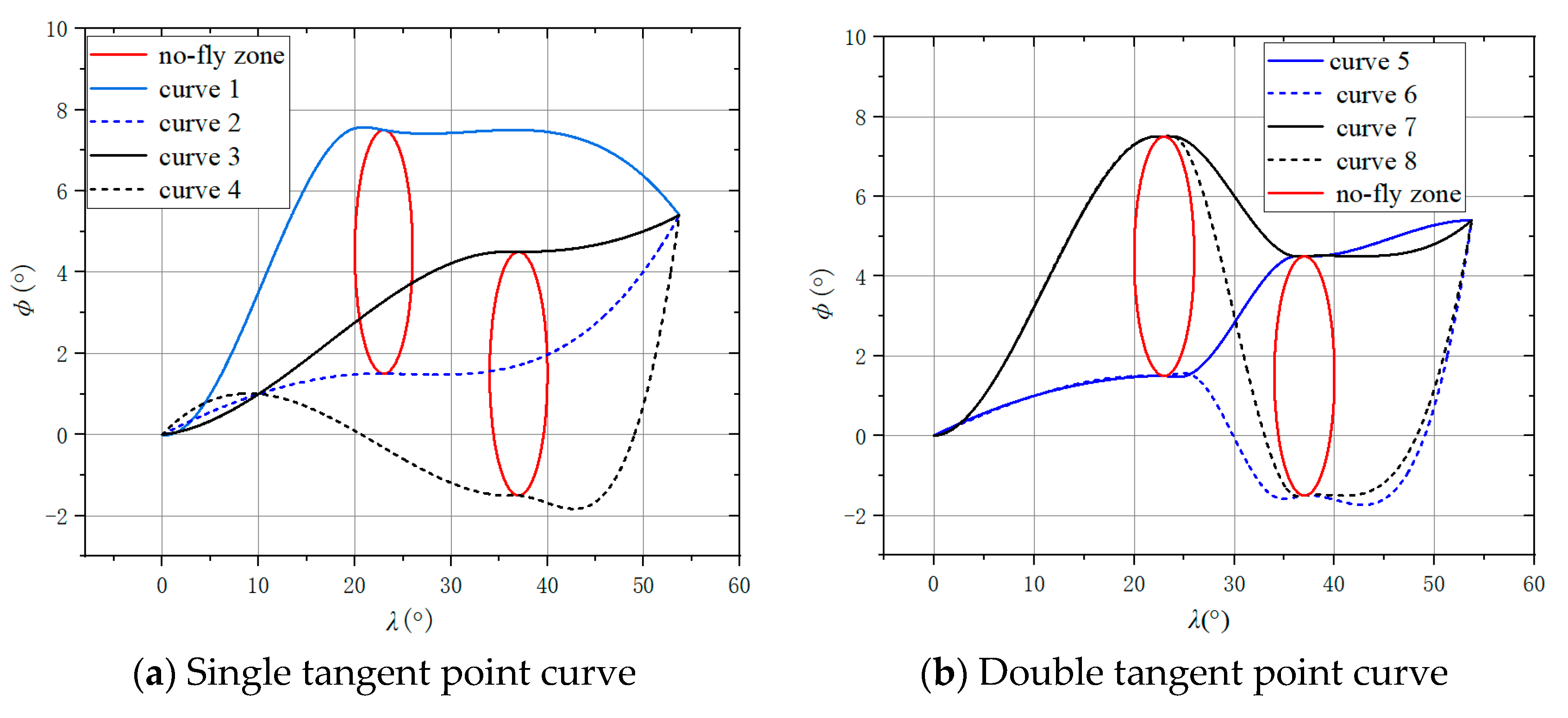
Based on the method in section 3.2. The evaluation function J of these 8 trajectories is shown in Table 1. All curves generated by single and double tangent points are shown in Figure 11 respectively.

It can be seen that both single and double tangent points generate 4 curves, and the trajectory 5 is obtained as the optimal solution, and the augmented and simplified points are shown in Table 2.

Now, the path points required for trajectory planning are obtained.

5.3. Simulation of Network Training

1.

DNN network training

Set the maximum number of iterations of network training to 1000, the minimum performance gradient to 10^-7, the maximum number of confirmed failures to 6, the target value of error limit to 0, and the learning rate to 0.05. The parameter settings in the reward value function are shown in Table 3.

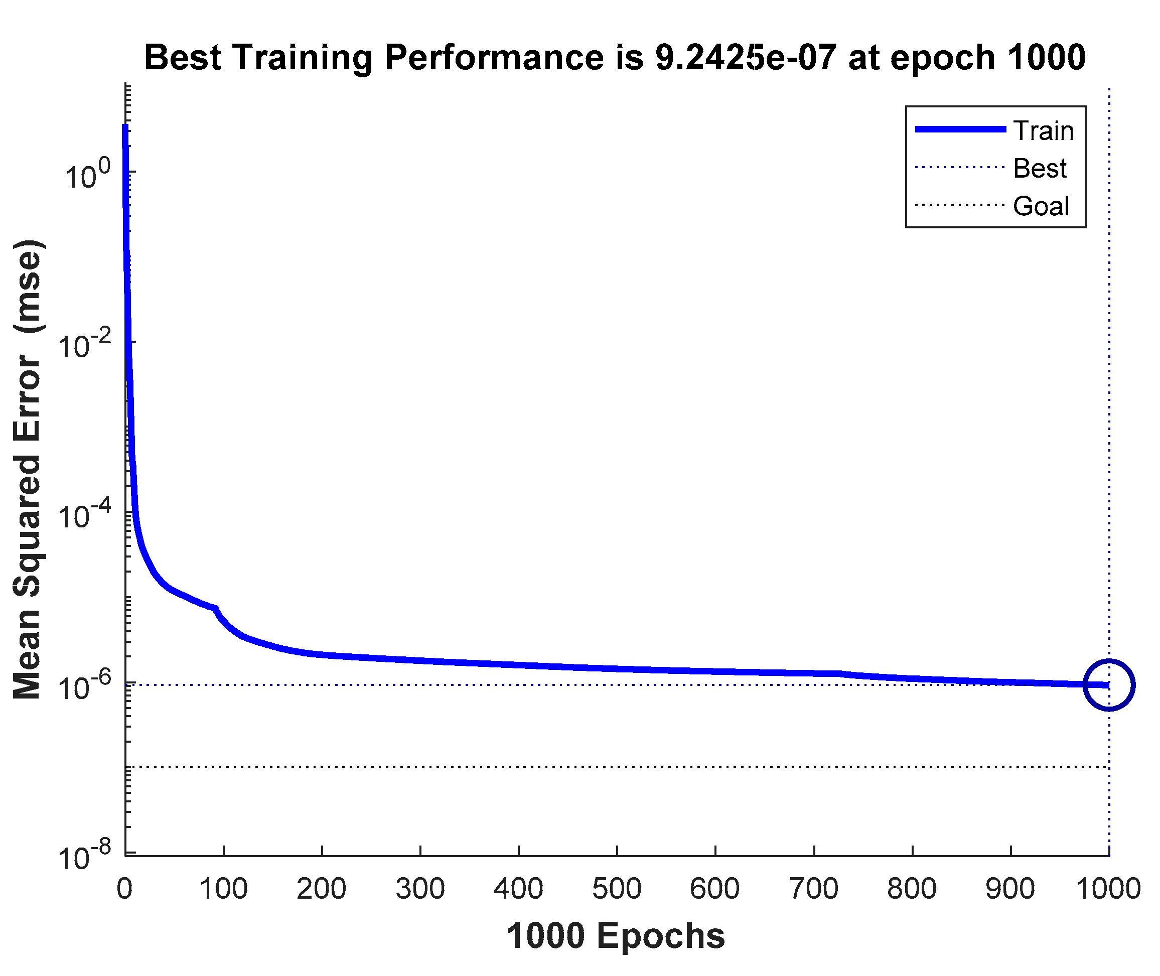
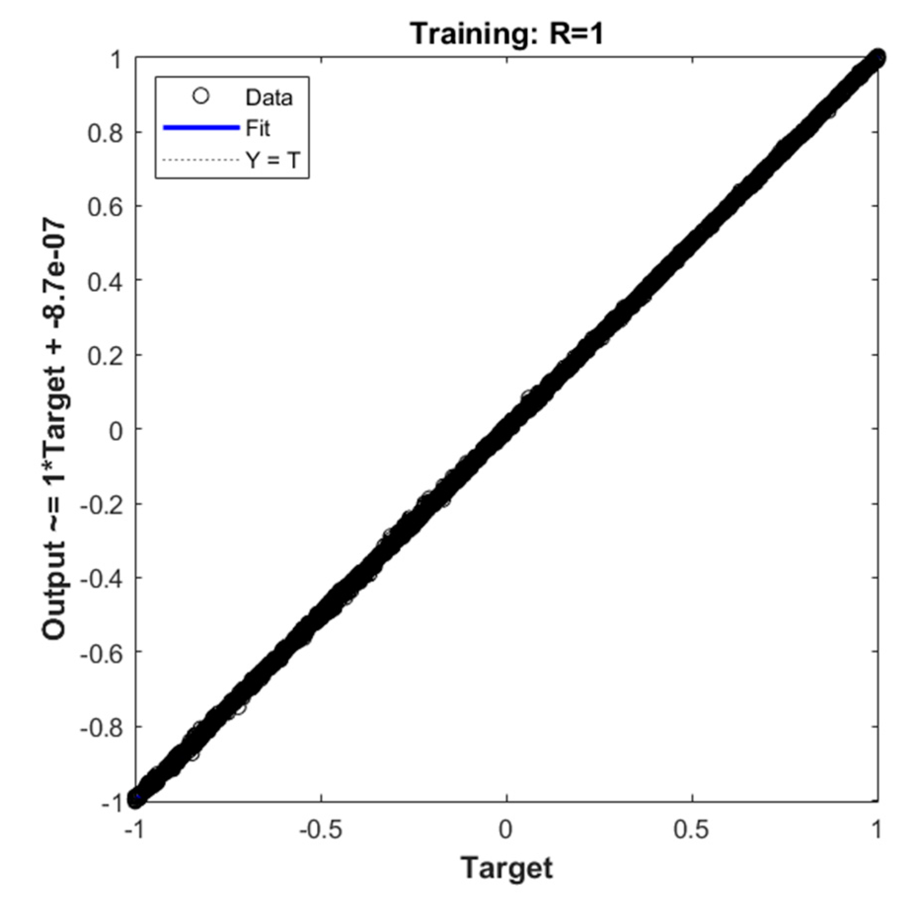
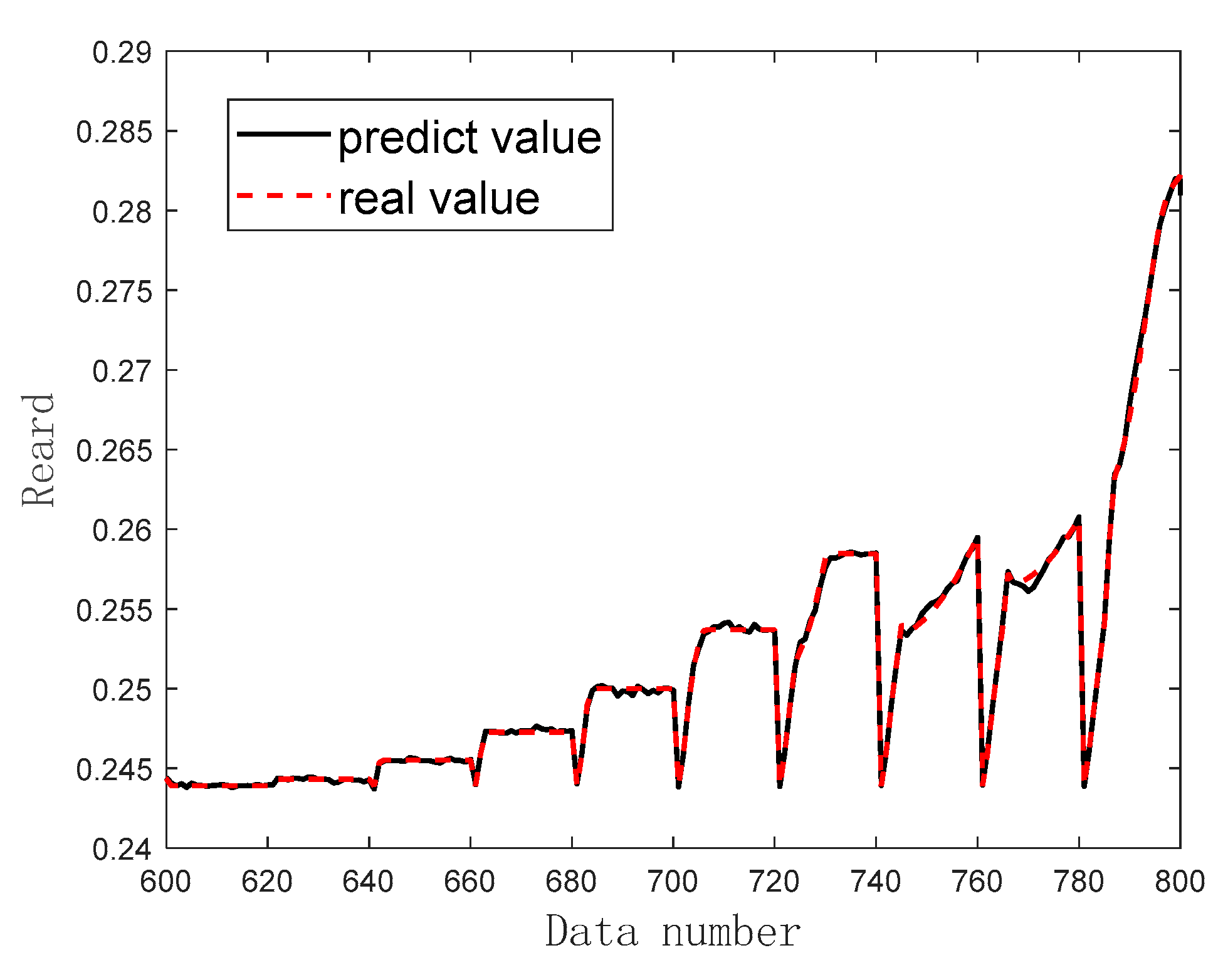
The learning effect of the training process is shown in Figure 12 and Figure 13. Part of the sample (group 600 to group 800 data) was randomly selected for testing, and the test results were compared with the sample results, as shown in Figure 14.

From the above results, it can be seen that when the number of iterations reaches 1000, the mean square error of the network converges to 9.2425×10-7, which meets the requirement. The sample regression performance indicator R=1 indicates strong data regression. As shown in Figure 14, the test results basically coincide with the sample. The above results demonstrate the good fitting ability of DNN, which can achieve accurate and fast estimation of the rewards.

Figure 12. Mean squared error.

Figure 12. Mean squared error.

Figure 13. Sample regression curve.

Figure 13. Sample regression curve.

Figure 14. Comparison of Test and Samples Reward.

Figure 14. Comparison of Test and Samples Reward.

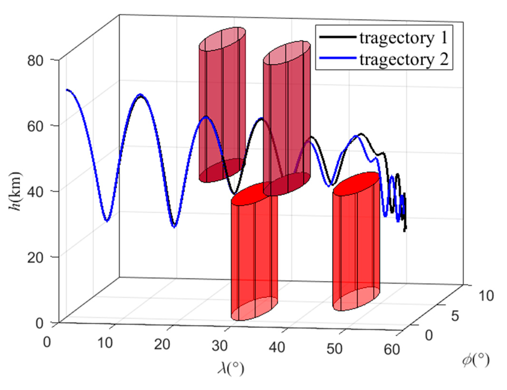
5.4. Simulation of trajectory planning algorithm

Figure 16. 3-D trajectory.

Figure 16. 3-D trajectory.

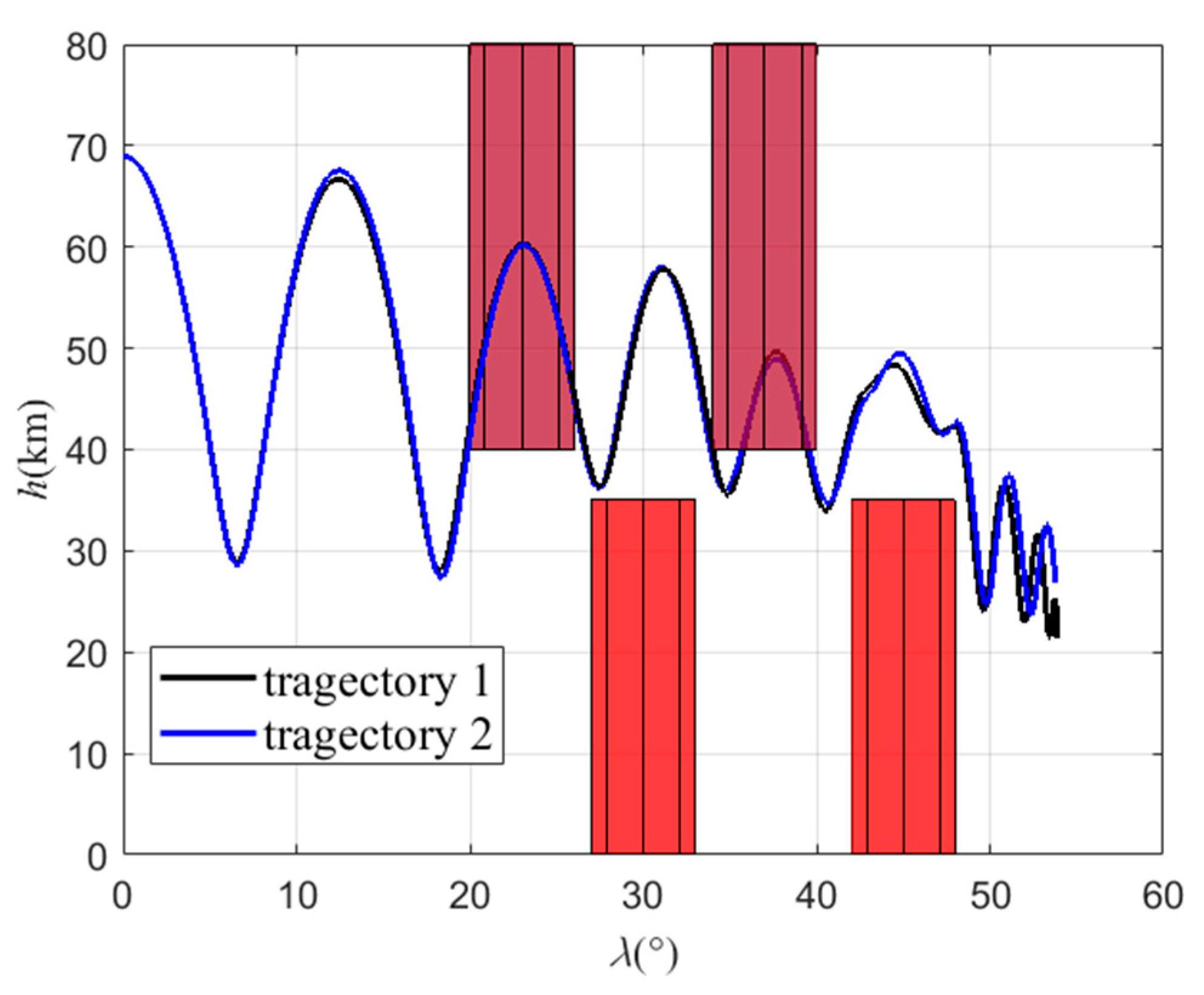
Figure 17. Longitudinal trajectory.

Figure 17. Longitudinal trajectory.

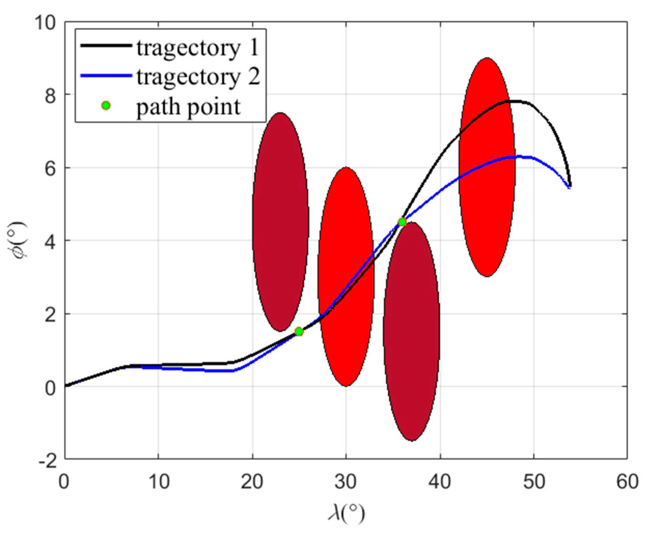
Figure 18. Lateral trajectory.

Figure 18. Lateral trajectory.

Figure 19. Pitch angle curve.

Figure 19. Pitch angle curve.

Figure 20. Speed curve.

Figure 20. Speed curve.

Figure 21. Path angle curve.

Figure 21. Path angle curve.

Figure 22. Heading angle curve.

Figure 22. Heading angle curve.

Figure 23. H-V profile.

Figure 23. H-V profile.

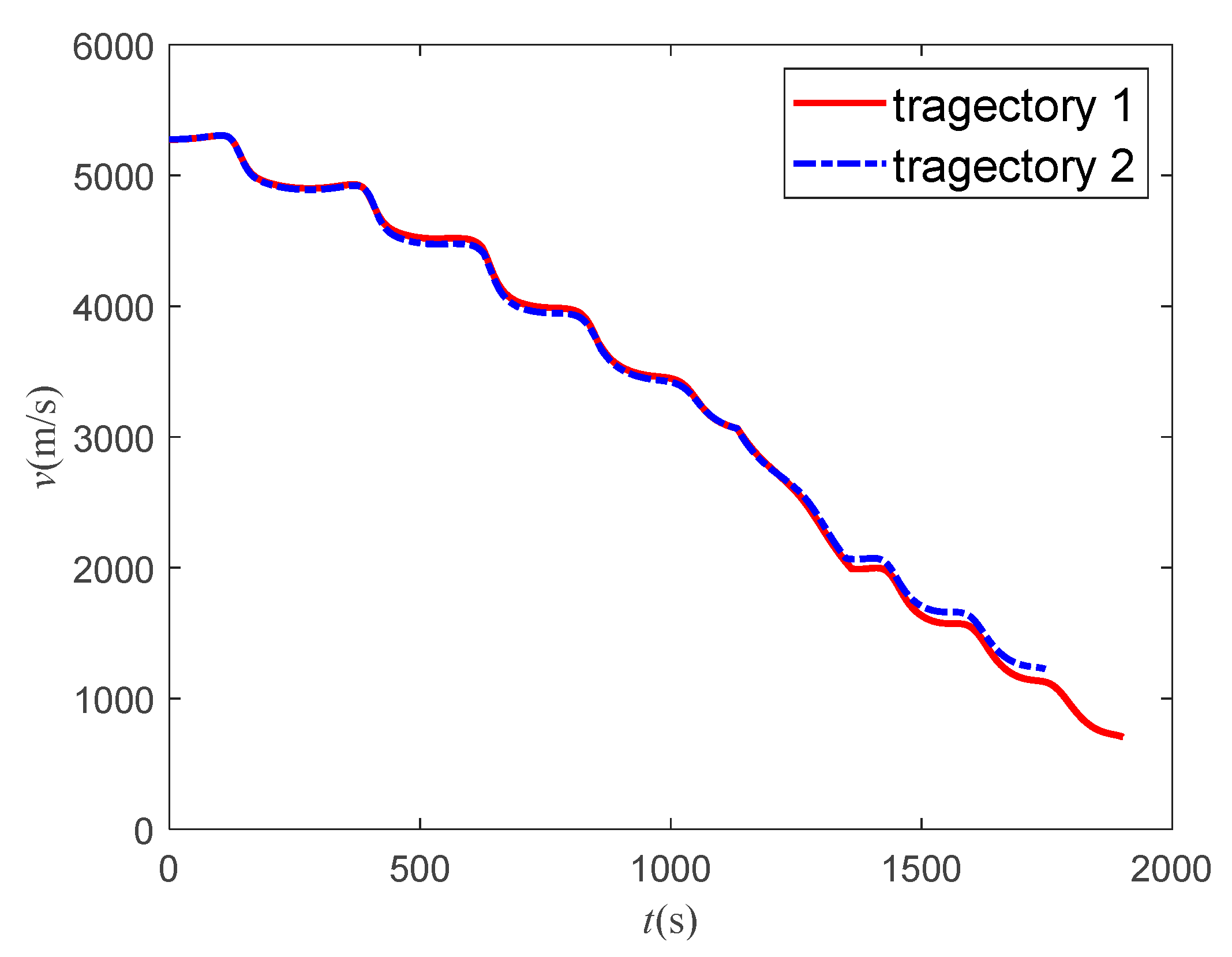
According to the 3-D, longitudinal and lateral trajectory, the aircraft can reach target using both methods. And it can cross two type 2 zones (light red) from the top and avoid two type 1 zones (dark red) from the side, which indicates the effectiveness of the attack and sweep angle scheme, path point scheme and bank angle scheme. The improved method has a shorter trajectory. In both cases, the improvement method takes less time. 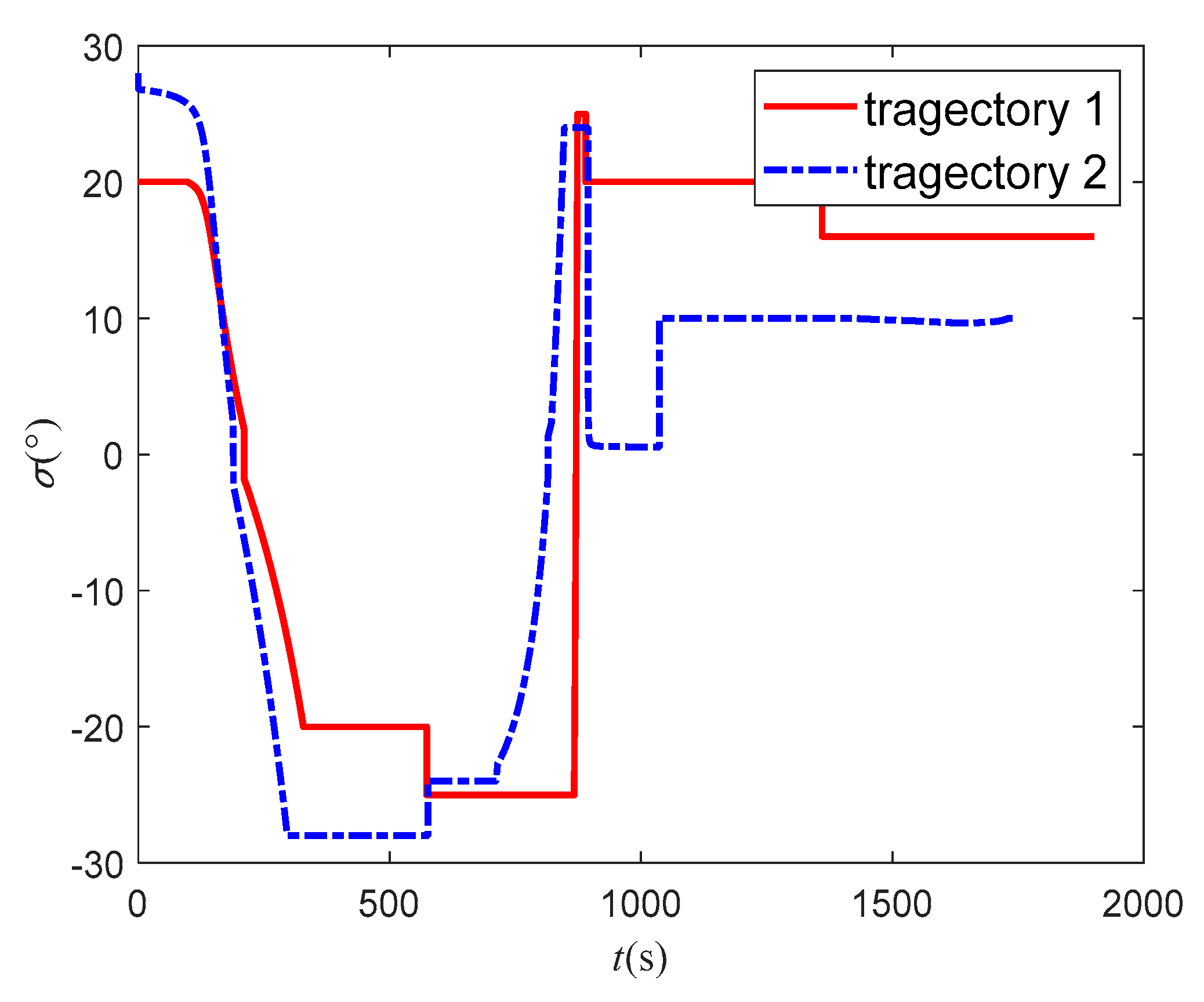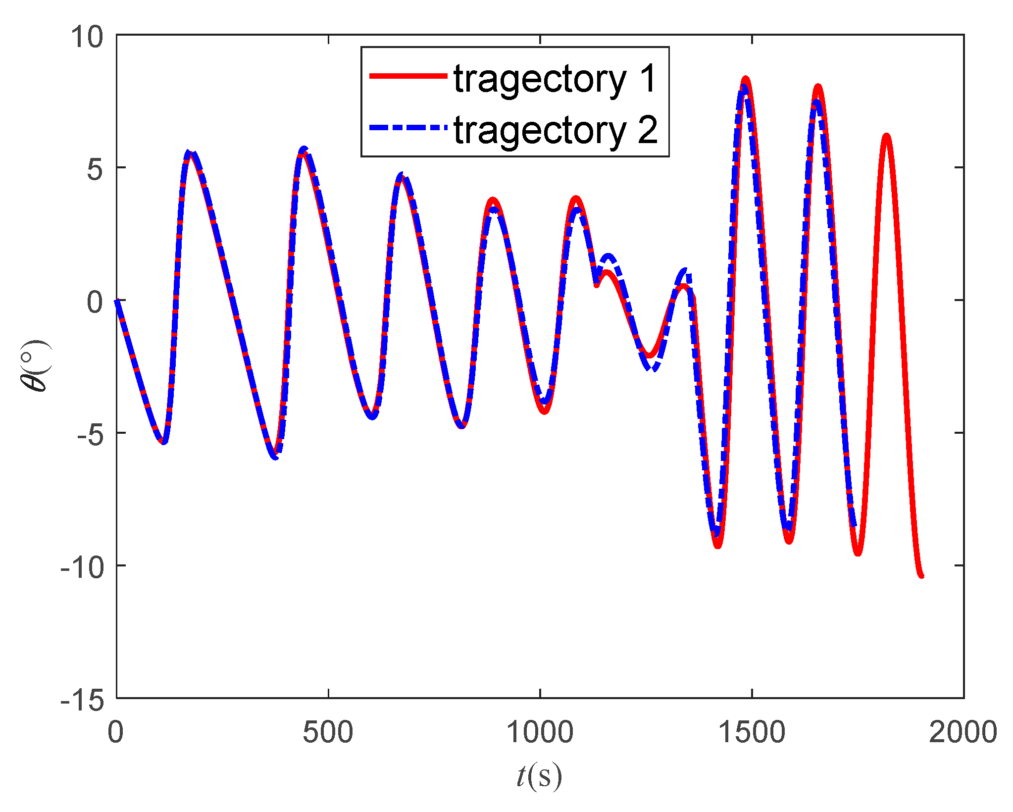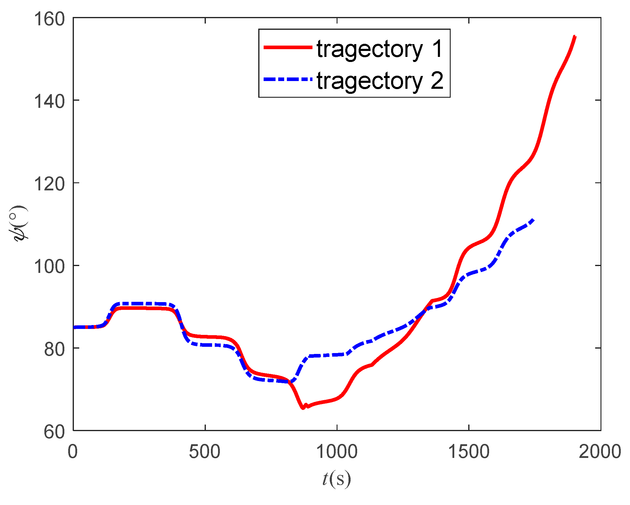Figure 19 are the bank angle curves, which shows that there is a difference between the two methods. It can be considered that the improving method is an optimal solution of the basic method. The basic method is to set a gradient optimization artificially and output the result as long as the aircraft reaches target. In the process of reinforcement learning, the whole process is considered to be optimal, so its trajectory is better. Due to the same longitudinal command, the flight path angles of the two trajectories are almost the same. The difference of bank angle makes the heading angle vary greatly. The change of the heading angle of the basic method is larger, which indicates the advantage of the improved method. 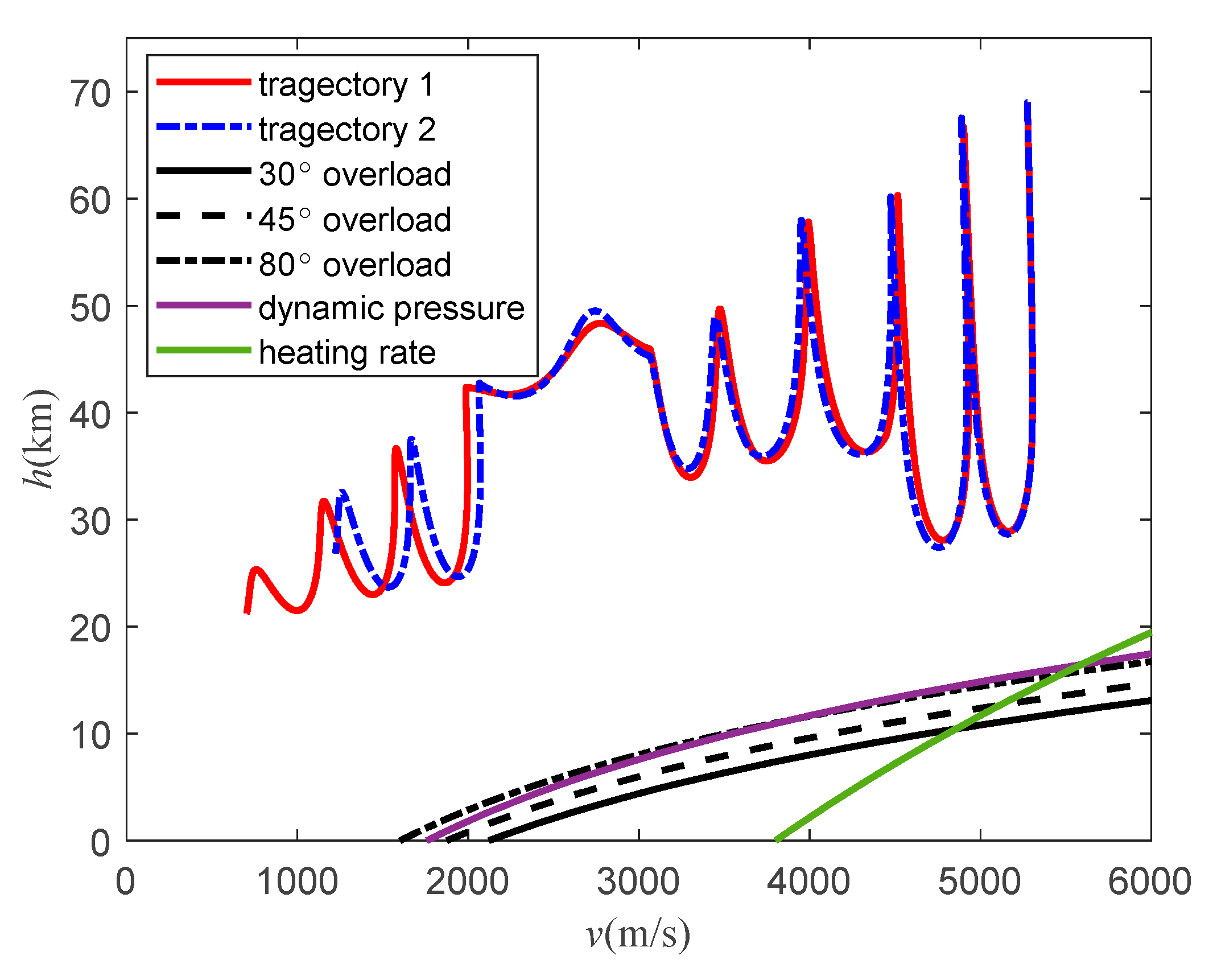According to the h-v flight profile in Figure 23, it can be seen that the h-v curves of the aircraft are all above the three overloads, heating rate, and dynamic pressure curves, indicating that the trajectories obtained by both methods meet the performance constraints of the aircraft. And the improved method obtains a better end state for the trajectory.

6. Conclusions

This article aiming at the trajectory safety planning of hypersonic morphing vehicle, designed a trajectory planning algorithm by using the predictor-corrector method, including the basic algorithm and the improved algorithm. In the basic algorithm, Q-learning is used to obtain the attack and sweep angle scheme, B-spline curve is used to obtain the flight path point, and the bank angle scheme is designed. The basic algorithm can ensure that the aircraft can avoid the no-fly zones from the longitudinal and lateral respectively, and reach the target point safely. In the improved algorithm, MCRL is used to improve predictor-corrector method and DNN is used to fit reward. The improved method produces a better trajectory while ensuring safe flight and reaching the target. Simulation results show the effectiveness of algorithm.

References

- Jason Bowman, Ryan Plumley, Jeffrey Dubois and David Wright. "Mission Effectiveness Comparisons of Morphing and Non-Morphing Vehicles," AIAA 2006-7771. 6th AIAA Aviation Technology, Integration and Operations Conference (ATIO). September 2006. https://doi.org/10.2514/6.2006-7771. [CrossRef]
- Austin, A. Phoenix, Jesse R. Maxwell, and Robert E. Rogers. "Mach 5–3.5 Morphing Wave-rider Accuracy and Aerodynamic Performance Evaluation". Journal of Aircraft, 2019 56:5, 2047-2061.
- W. Peng, Z. Feng, T. Yang and B. Zhang, "Trajectory multi-objective optimization of hypersonic morphing aircraft based on variable sweep wing," 2018 3rd International Conference on Control and Robotics Engineering (ICCRE), Nagoya, Japan, 2018, pp. 65-69.
- H. Yang, T. Chao and S. Wang, "Multi-objective Trajectory Optimization for Hypersonic Telescopic Wing Morphing Aircraft Using a Hybrid MOEA/D," 2022 China Automation Congress (CAC), Xiamen, China, 2022, pp. 2653-2658.
- C Wei, X Ju, F He and B G Lu. "Research on Non-stationary Control of Advanced Hypersonic Morphing Vehicles," AIAA 2017-2405. 21st AIAA International Space Planes and Hypersonics Technologies Conference. March 2017. [CrossRef]
- J. Guo, Y. Wang, X. Liao, C. Wang, J. Qiao and H. Teng, "Attitude Control for Hypersonic Morphing Vehicles Based on Fixed-time Disturbance Observers," 2022 China Automation Congress (CAC), Xiamen, China, 2022, pp. 6616-6621. [CrossRef]
- Wingrove, R. C. (1963). Survey of Atmosphere Re-entry Guidance and Control Methods. AIAA Journal, 1(9), 2019–2029. [CrossRef]
- Mease K, Chen D, Tandon S, et al. A three-dimensional predictive entry guidance approach [C]. AIAA Guidance, Navigation and Control Conference and Exhibit. American Institute of Aeronautics and Astronautics, 2000.
- H.L. Zhao and H. W. Liu, "A Predictor-corrector Smoothing Newton Method for Solving the Second-order Cone Complementarity," 2010 International Conference on Computational Aspects of Social Networks, Taiyuan, China, 2010, pp. 259-262. [CrossRef]
- H. Wang, Q. Li and Z. Ren, "Predictor-corrector entry guidance for high-lifting hypersonic vehicles," 2016 35th Chinese Control Conference (CCC), Chengdu, China, 2016, pp. 5636-5640. [CrossRef]
- S. Liu, Z. Liang, Q. Li and Z. Ren, "Predictor-corrector guidance for entry with terminal altitude constraint," 2016 35th Chinese Control Conference (CCC), Chengdu, China, 2016, pp. 5557-5562. [CrossRef]
- M. Xu, L. Liu, G. Tang and K. Chen, "Quasi-equilibrium glide auto-adaptive entry guidance based on ideology of predictor-corrector," Proceedings of 5th International Conference on Recent Advances in Space Technologies - RAST2011, Istanbul, Turkey, 2011, pp. 265-269.
- W Li, S Sun and Z Shen, "An adaptive predictor-corrector entry guidance law based on online parameter estimation," 2016 IEEE Chinese Guidance, Navigation and Control Conference (CGNCC), Nanjing, 2016, pp. 1692-1697. [CrossRef]
- Z. Liang, Z. Ren, C. Bai and Z. Xiong, "Hybrid reentry guidance based on reference-trajectory and predictor-corrector," Proceedings of the 32nd Chinese Control Conference, Xi'an, China, 2013, pp. 4870-4874.
- Jay W. McMahon, Davide Amato, Donald Kuettel and Melis J. Grace. "Stochastic Predictor-Corrector Guidance," AIAA 2022-1771. AIAA SCITECH 2022 Forum. January 2022. 20 January. [CrossRef]
- H. Chi and M. Zhou, "Trajectory Planning for Hypersonic Vehicles with Reinforcement Learning," 2021 40th Chinese Control Conference (CCC), Shanghai, China, 2021, pp. 3721-3726. [CrossRef]
- Z. Shen, J. Yu, X. Dong and Z. Ren, "Deep Neural Network-Based Penetration Trajectory Generation for Hypersonic Gliding Vehicles Encountering Two Interceptors," 2022 41st Chinese Control Conference (CCC), Hefei, China, 2022, pp. 3392-3397.
- Z. Kai and G. Zhenyun, "Neural predictor-corrector guidance based on optimized trajectory," Proceedings of 2014 IEEE Chinese Guidance, Navigation and Control Conference, Yantai, China, 2014, pp. 523-528. [CrossRef]
- Y. Lv, D. Hao, Y. Gao and Y. Li, "Q-Learning Dynamic Path Planning for an HCV Avoiding Unknown Threatened Area," 2020 Chinese Automation Congress (CAC), Shanghai, China, 2020, pp. 271-274. [CrossRef]
- Brian Gaudet, Kris Drozd and Roberto Furfaro. "Adaptive Approach Phase Guidance for a Hypersonic Glider via Reinforcement Meta Learning," AIAA 2022-2214. AIAA SCITECH 2022 Forum. January 2022. [CrossRef]
- J. Subramanian and A. Mahajan, "Renewal Monte Carlo: Renewal Theory-Based Reinforcement Learning," in IEEE Transactions on Automatic Control, vol. 65, no. 8, pp. 3663-3670, Aug. 2020.
- J. F. Peters, D. Lockery and S. Ramanna, "Monte Carlo off-policy reinforcement learning: a rough set approach," Fifth International Conference on Hybrid Intelligent Systems (HIS'05), Rio de Janeiro, Brazil, 2005, pp. 6.
- Rory Lipkis, Ritchie Lee, Joshua Silbermann and Tyler Young. "Adaptive Stress Testing of Collision Avoidance Systems for Small UASs with Deep Reinforcement Learning," AIAA 2022-1854. AIAA SCITECH 2022 Forum. January 2022. [CrossRef]
- Abhay Singh Bhadoriya, Swaroop Darbha, Sivakumar Rathinam, David Casbeer, Steven J. Rasmussen and Satyanarayana G. Manyam. "Multi-Agent Assisted Shortest Path Planning using Monte Carlo Tree Search," AIAA 2023-2655. AIAA SCITECH 2023 Forum. January 20233. [CrossRef]
- Lu, Ping. "Entry Guidance: A Unified Method". Journal of Guidance, Control, and Dynamics, 37(3), 713–728. [CrossRef]
- P. Han and J. Shan, "RLV's re-entry trajectory optimization based on B-spline theory," 2011 International Conference on Electrical and Control Engineering, Yichang, China, 2011, pp. 4942-4946.
- E. Adsawinnawanawa and N. Keeratipranon, "The Sharing of Similar Knowledge on Monte Carlo Algorithm applies to Cryptocurrency Trading Problem," 2022 International Electrical Engineering Congress (iEECON), Khon Kaen, Thailand, 2022, pp. 1-4. [CrossRef]