
Submitted:
26 July 2023
Posted:
27 July 2023
You are already at the latest version
Abstract
Remote sensing (RS) technology has significantly contributed to geological exploration and mineral resource assessment. However, its effective application in vegetated areas encounters various challenges. This paper aims to provide a comprehensive overview of the challenges and opportunities associated with RS-based lithological identification in vegetated regions. The article begins by introducing the sources and processing methods of RS data, which serve as the foundation for subsequent analysis. Moreover, it highlights the techniques and methodologies employed for lithological classification in vegetated areas. Notably, hyperspectral RS and Synthetic Aperture Radar (SAR) have emerged as prominent tools in lithological identification. In addition, this paper addresses the limitations inherent in RS technology, including issues related to vegetation cover and terrain effects, which significantly impact accurate lithological mapping. To propel further advancements in the field, the paper proposes promising avenues for future research and development. These include the integration of multi-source data to enhance classification accuracy and the exploration of novel RS technologies and algorithms. In summary, this paper presents valuable insights and recommendations for advancing the study of RS-based lithological identification in vegetated areas.
Keywords:
Lithology Mapping
; Machine Learning
; Deep Learning
; Feature Extraction
; Remote Sensing
; Vegetated area
1. Introduction
Accurate lithological mapping is essential in geological surveys and mineral resource exploration [1,2,3,4]. Rocks are classified into sedimentary, magmatic, and metamorphic types based on their formation process, with detailed subtypes referenced in [5,6,7,8]. Leveraging the distinctive spectral responses and texture information of rocks, remote sensing (RS) data/technology facilitates rapid geological mapping [9]. However, the detection of rock information in vegetated areas poses challenges due to weak signals and interference from vegetation cover. Even with vegetation cover of just over 10%, subsurface information can be greatly obscured or entirely hidden [10,11]. Consequently, the extraction of lithologic information in vegetated areas represents a significant obstacle in current geological applications [12].
Various approaches have been identified to address vegetation obstruction in lithological RS. In the field of vegetation-based lithological mapping, classification methods can be categorized into three primary approaches. The first approach focuses on re-emerging lithological information through Vegetation Suppression Method (VSM) [13,14]. The second approach utilizes Spectral Mixing Analysis (SMA) to decompose and extract target information, specifically lithological categories [15,16]. The third approach involves indirect classification utilizing a range of algorithms, such as maximum likelihood classification (MLC) [17], Support Vector Machines (SVM) [18], Random Forest (RF) [19], Artificial Neural Networks (ANN) [20,21,22], and deep learning algorithms (DLAs) [23,24], significantly facilitating the process of indirect lithological identification with development of ML.
In recent years, the field of lithological identification has benefited from advancements in artificial intelligence and the availability of diverse RS datasets. Among these datasets, the Landsat series satellites have emerged as the primary choice for researchers in vegetation-based lithological mapping studies [25,26,27,28]. Their high cost-effectiveness, wide coverage, and high spatial resolution effectively indicate vegetation and lithology-soil information, providing a solid foundation for lithological identification. However, it is important to note that the accuracy of information extraction is constrained by the mixed pixel phenomenon and the loss of information resulting from the low spatial resolution [29]. Furthermore, the emergence of high-resolution imagery has attracted geologists' attention. Advanced Space Borne Thermal Emission and Reflection Radiometer (ASTER) with multi-spectral (15m) and thermal infrared (TIR) (30m) data [30,31] allow for the extraction of spectral and thermal features for surface lithology analysis. Sentinel-2[32] provides high spatial resolution multi-spectral data (up to 10m), which is suitable for large-scale lithological identification. Additionally, WorldView-3[33] and WorldView-4 offer high-resolution multi-spectral and TIR imagery, enabling the capture of surface details and spectral characteristics. Advanced hyperspectral sensors like Earth Observing-1 (EO-1) [34], PRISMA [35], EnMAP [36], and HyspIRI [37] provide a wider spectral range and finer resolution, facilitating precise lithological identification and mineral analysis. Moreover, China's high-resolution satellites, including Zhongzi Resources Satellite-1 (ZY-1) [38], ZY-3[39], and the Gaofen series (GF) [40,41], cover visible (VIR), near-infrared (NIR), and mid-infrared spectra, thereby establishing a robust data foundation for detailed localized lithological survey research.
Despite the notable advancements of optical sensors in lithological identification, they still face certain challenges. Multispectral images are susceptible to various factors such as lighting and weather conditions, spectral resolution limitations, and the complex nature of geological units [23,29]. Similarly, high-resolution hyperspectral images are prone to spectral confusion, complexities in data processing and analysis, and atmospheric interference [35]. In contrast, SAR technology can address some of these challenges and offers advantages, including weather independence, detailed capture of texture features, and high sensitivity to surface physical properties [42]. The C-band provides high spatial resolution, capturing microscopic rock structure details and reflecting subtle lithological variations and reflectivity differences [43,44]. On the other hand, the L-band has the capability to penetrate vegetation and shallow surface coverings, directly acquiring information about subsurface rocks [45]. Sentinel-1[46], polarimetric SAR (Pol-SAR) [47] and Phased Array type L-band SAR (PALSAR) [45,48] are highly favored for lithological mapping. However, studies have shown that radar data generally has lower spatial resolution compared to optical images, and the acquisition and processing of radar data can be complex [45]. Therefore, relying solely on SAR data for lithological discrimination may lead to poorer performance [44].
The challenge in lithological mapping in vegetated areas lies in the inability of a single type of data resource to accurately diagnose the characteristics of all rock units [23]. Considering the correlation between lithology and factors such as vegetation [20,49], topography [22,50], temperature [51], humidity [52], etc., indirect lithological identification can be achieved through multi-source RS techniques or integrating RS with ancillary data [53,54]. This strategy has been widely employed in practical geological research and resource exploration, leading to remarkable achievements [13,15,20,42,55]. It is worth noting that the fusion of multi-source data generates high-dimensional features with numerous variables. However, using all these variables can pose computational challenges for MLAs and may not always yield satisfactory results [56,57] due to some variables are highly correlated, noisy, redundant, or irrelevant [58]. Therefore, selecting optimal feature variables is crucial for achieving satisfactory classification outcomes. For specific methods, please consult relevant literature [59,60]. The significance of this process has been highlighted in previous research [28].
The aim of this paper is to provide theoretical, technical, and methodological support for further lithology mapping work in vegetation-covered areas by summarizing existing research conducted by previous scholars. In Section 2, we discuss data preparation, including RS data such as optical, hyperspectral and radar imagery. Section 3 covers feature extraction and classification methods. Section 4 provides an in-depth analysis of the related studies on rock classification in vegetation-covered areas. In Section 5, we discussed and anticipated the opportunities and future development in the research field of vegetation-based lithological mapping. Moving on to Section 6, we provide a comprehensive summary of the research and shed light on the challenges encountered in the field of lithological mapping.
2. RS Imagery
2.1. Optical Imagery
The Landsat series of satellites, operated jointly by the National Aeronautics and Space Administration (NASA) and the United States Geological Survey (USGS)[61,62], comprises Earth observation satellites equipped with multiple multispectral sensors, including Multi-Spectral Scanner (MSS) aboard Landsat 1-5[63], Thematic Mapper (TM) aboard Landsat 4 and 5[27,64], Enhanced Thematic Mapper Plus (ETM+) aboard Landsat 7[65], Operational Land Imager (OLI) and Thermal Infrared Sensor (TIRS) aboard Landsat 8[66], Operational Land Imager 2 (OLI-2) and TIRS-2 aboard Landsat 9[67]. These satellites, spanning from 1972 to the present (excluding a failed launch), capture visible, near-infrared, mid-infrared, and thermal-infrared spectra, providing valuable and abundant data for lithological mapping. Landsat 8 and Landsat 9 are the latest satellites in the series. Launched on February 11, 2013, Landsat 8 carries OLI and TIRS sensors, enabling the capture of visible, short-wave infrared, and TIR radiation [68]. Compared to previous satellites, Landsat 8 provides more accurate and detailed data, as observed by Mwaniki [69], who found that OLI performs better than ETM+ in distinguishing different lithological units.
Freely available Landsat data, including the latest Landsat 9, is a crucial tool for Earth sciences, resource exploration, and environmental monitoring, thanks to its global coverage, long-term time series, and multispectral information. Launched on September 27, 2021, and operational since 2023, Landsat 9 utilizes the OLI-2 and TIRS-2 sensors to capture data in the visible, infrared, and TIR spectra, providing high-resolution and multispectral capabilities for Earth observation [67]. Research by You [70] shows that Landsat 9 outperforms Landsat 8 in water body and tree species classification, attributed to its increased radiometric resolution from 12 bits (Landsat 8) to 14 bits, improving sensitivity to brightness and color and enabling the detection of subtle differences, particularly in darker areas like water bodies. However, as a new satellite, Landsat 9 may present uncertainties and challenges related to data quality, sensor performance, and data processing algorithms [70].
In the aftermath of the data gaps in Landsat imagery caused by ETM+ scan line corrector failures in June 2003 [71], ASTER (Advanced Spaceborne Thermal Emission Reflection Radiometer) has emerged as a reliable substitute for TIR imagery. ASTER comprises a visible and near-infrared subsystem, a shortwave infrared radiometer, and a TIR radiometer [72]. Please refer to Table 2 for specific band information. The availability of this data has provided robust support for lithological mapping research [30,31,65,73,74]. Moreover, the global digital elevation model data derived from ASTER stereo image pairs, known as the ASTER GDEM (Shuttle Radar Topography Mission Global Digital Elevation Model), can be effectively utilized for band georeferencing, calibration, and shading calculations [75].

Table 1.
Band (B), wavelength (WL), and resolution (R) information of Landsat (L) 4-5/7/8/9, modified from [27,67,70].
| 9 | WL(µm) | R(m) | L7 | WL(µm) | R(m) | L8 | WL(µm) | R(m) | L9 | WL(µm) | R(m) |
|---|---|---|---|---|---|---|---|---|---|---|---|
| B 1 | 0.43–0.45 | 30 | B 1 | 0.43–0.45 | 30 | ||||||
| B 1 | 0.45-0.52 | 30 | B 1 | 0.45-0.52 | 30 | B 2 | 0.45–0.51 | 30 | B 2 | 0.45–0.51 | 30 |
| B 8 | 0.52-0.90 | 15 | B 3 | 0.53–0.59 | 30 | B 3 | 0.53–0.59 | 30 | |||
| B 2 | 0.52-0.60 | 30 | B 2 | 0.52-0.60 | 30 | B 4 | 0.64–0.67 | 30 | B 4 | 0.64–0.67 | 30 |
| B 3 | 0.63-0.69 | 30 | B 3 | 0.63-0.69 | 30 | B 5 | 0.85–0.88 | 30 | B 5 | 0.85–0.88 | 30 |
| B 4 | 0.76-0.90 | 30 | B 4 | 0.77-0.90 | 30 | Bd 6 | 1.57–1.65 | 30 | B 6 | 1.57–1.65 | 30 |
| B 7 | 2.11–2.29 | 30 | B 7 | 2.11–2.29 | 30 | ||||||
| B 5 | 1.55-1.75 | 30 | B 5 | 1.55-1.75 | 30 | B 8 | 0.50–0.68 | 15 | B 8 | 0.50–0.68 | 15 |
| B 7 | 2.08-2.35 | 30 | B 7 | 2.08-2.35 | 30 | B 9 | 1.36–1.38 | 30 | B 9 | 1.36–1.38 | 30 |
| B 6 | 10.40-12.50 | 120*(30) | B 6 | 10.40-12.50 | 60*(30) | B 10 | 10.60-11.19 | 100 | B 10 | 10.60-11.19 | 100 |
| Band 11 | 11.50-12.51 | 100 | B 11 | 11.50-12.51 | 100 |
Although the aforementioned data has been widely used and has achieved significant progress, it lacks the capability to meet the requirements of fine-scale lithological classification studies at a local level. The Sentinel series of satellites offers reliable data sets for the Copernicus program, facilitating real-time dynamic monitoring of the global environment and security [77]. The Sentinel-2 satellite constellation [78], consisting of Sentinel-2A and Sentinel-2B launched by the European Space Agency (ESA) on June 23, 2015, and March 7, 2017, respectively, offers a valuable alternative to address this limitation. Sentinel-2 provides coverage between latitudes 56°S and 84°N, with a revisit period of 5 days at the equator and a swath width of 290 kilometers [32]. For specific band information, please refer to Table 3. Sentinel-2's advantages, such as higher spatial and spectral resolution, short revisit period, more bands, and open data access, make it essential for land cover classification and lithological mapping [23,29,55]. However, it's large data volume necessitates extensive processing and storage, placing significant demands on computing and storage resources [55]. Therefore, a comprehensive consideration of these factors is crucial when utilizing this data.
WorldView-3 (WV-3) [33] is a commercial high-resolution satellite operated by Digital Globe. Launched on August 13, 2014, it provides exceptional image data with outstanding spatial resolution. With a spatial resolution of 0.31 meters (31 centimeters) in PAN band, 1.24 meters in MS (including blue, green, red, NIR) and 3.7 meters in SWIR [80], WV-3 stands out for its remarkable spatial capabilities. The combination of high spectral and spatial resolution empowers WV-3 to excel in lithological mapping, delivering precise and comprehensive information about rock types [40,80].
2.2. Hyperspectral Imagery
Hyperspectral imagery offers advantages such as high spectral resolution, multi-band coverage, spectral continuity, spectral unmixing capability, and feature discrimination ability. It is widely used for lithological classification in vegetated areas with satellites like EO-1[34], PRISMA [35], EnMAP [36], Hyperion [16], and HyspIRI [37]. A comprehensive review paper on the applications of hyperspectral images in lithological mapping, mineral exploration, and environmental geology was found during the literature review s[81]. The paper provides an extensive overview of hyperspectral missions, spectral properties of diagnostic minerals, and techniques for geologic information extraction from spaceborne/airborne hyperspectral images. Hence, we will not delve further into data details. However, it is important to acknowledge some limitations of hyperspectral imagery, including limited data availability [16] and coverage, as well as lower spatial resolution compared to multispectral imagery [81].
2.3. Radar Data
Sentinel-1 is a SAR satellite developed by the European Space Agency (ESA) and forms part of a two-satellite Earth observation system [46]. It consists of two satellites named S1A and S1B launched on April 3, 2014 and April 25, 2016, respectively [44]. S1 utilize radar systems operating in the C-band and X-band, enabling the capture of surface information regardless of weather conditions, including topography, geomorphology, land cover, and surface changes. Notably, they offer high resolution (up to 5 meters), multipolarization (VV, VH, HH, and HV), multiple modes, wide swath coverage, and frequent revisit periods. However, practical applications necessitate consideration of data storage and processing concerns [44,82]. Moreover, SAR data's sensitivity to surface roughness [78] often requires integration with other data sources such as optical imagery and terrain data for interpretation [82].
ALOS-PALSAR [83] (Phased Array L-type band SAR), mounted on Advanced Land Observing Satellite (ALOS) by the Japan Aerospace Exploration Agency (JAXA), is a SAR sensor with comparable lithological mapping performance to Sentinel-1 (C-band) [45]. ALOS-PALSAR provides high-resolution radar imagery and digital elevation model (DEM) data, which are used for applications such as land cover classification, terrain measurement, and underground target detection. Operating in the L-band (1.27 GHz), ALOS-PALSAR features dual polarization (HH and HV), high resolution (1m), DEM, and multiple modes [83]. Combining it with optical RS and radar data enhances the accuracy and reliability of lithological classification [45].
Airborne laser detection and ranging (LiDAR) is an active RS technology that can acquire accurate and high-resolution terrain data, with a resolution of approximately 1-4 meters. This technology offers a potential solution to overcome ambiguous identification of the surface by dense vegetation schemes [84]. Laser reflections from the ground can be distinguished from vegetation reflections, allowing for precise DTM (Digital Terrain Model) generation. The ability to identify subtle topographical features in high-resolution DTMs makes LiDAR an important tool for lithology identification [28].
The C-band Spaceborne Imaging Radar and the X-band SAR instrument onboard the space shuttle are utilized for Shuttle Radar Topography Mission (SRTM), a mapping project conducted jointly by NASA and NGA (National Geospatial-Intelligence Agency) [42]. SRTM is renowned as one of the highest-resolution global digital elevation models accessible to the public, offering comprehensive global coverage, high resolution (ranging from 30 to 90 meters), and superior data quality. SRTM data is used in lithological identification studies, as factors like slope reflect rock erosion resistance [42]. However, the accuracy of SRTM is lower in polar and forest-covered regions due to SAR sensor characteristics, requiring caution in its use across different research areas.
Here, it is particularly important to mention that China's Gaofen, Huanjing and Ziyuan series satellites are notable sources of surface imagery data, offering spatial resolutions ranging from sub-meter to hundreds of meters. GF-1 [40,85]and GF-2[86], GF-3[86], GF-5[41,87], HJ-1A CCD [53], ZY-1 02D [38], and ZY-3[88], are widely utilized for lithological mapping, and their detailed specifications can be found in Table 4. Among them, GF-1, GF-2, HJ-1A CCD and ZY-3 loaded multispectral scanner, GF-5 and ZY-1 02D loaded hyperspectral scanner, and GF-3 loaded SAR camera. Their high spatial resolution enables accurate fine-scale lithological classification. However, it is crucial to consider that acquiring this data involves financial costs, and each satellite has its own strengths and limitations. For example, GF-2 excels in areas such as high spatial resolution, multiple spectral bands, and frequent revisit periods, but it has limitations in terms of coverage and relatively lower radiometric resolution, which may constrain certain fine-scale analysis applications [86]. Conversely, GF-3 offers benefits like multiple polarization modes and frequent revisit periods, but it has lower spatial resolution and a restricted number of spectral bands [86].
3. Method
3.1. Feature Extraction
Feature extraction is crucial in RS image classification and recognition. It converts raw pixel data into discriminative feature vectors [16], unveiling meaningful relationships [62] and patterns to enhance MLAs performance [40]. This chapter comprehensively reviews spectral features, terrain features and texture features used in constructing models for lithological mapping, providing detailed insights into their characteristics and applications.
3.1.1. Spectral Features
Reflectance/radiance characteristics play a crucial role in lithology mapping in vegetation-covered areas, utilizing various bands from optical imagery (VNIR, SWIR, and TIR) and radar data (C, L, and X bands). Optical bands such as VNIR and SWIR provide valuable information for rock identification based on color, reflectance, and absorption properties [16,23,24,29,75,89]. Additionally, TIR data aids in surface temperature inversion, revealing thermal characteristics and subsurface influences [90]. Temperature-related parameters like TVDI and other thermal features [91] can quantitatively assess land or rock properties. On the other hand, radar bands like X band offer insights into surface morphology and texture through surface and volume scattering, while C band penetrates vegetation and shallow soil, providing information about rock morphology and structure [44,45]. The longer wavelengths of the L band enable deeper penetration, facilitating echo signal analysis for lithology classification and geological structural analysis [44]. However, response characteristics in the L band may exhibit complexity and overlap among different lithology types [45].
Understanding the interplay between reflectance/radiance characteristics and lithology helps us comprehend the impact of lithology on aboveground plant communities in two key ways: nutrient provision for plant growth [92] and influence on water storage potential through weathering depth and porosity changes [93]. Variations in rock types across different regions with similar climates contribute to the formation of diverse plant communities [94]. Vegetation indices used in lithology mapping include NDVI, VIGS, and SWVI [28,75]. NDVI indicates vegetation coverage [78], VIGS detects vegetation stress from heavy metal elements [28], and SWVI reflects vegetation leaf water content [95].
Band ratio (BR) is widely used in lithological classification to differentiate different rock types by extracting various geological information through different combinations of bands [96]. For example, the Landsat TM [14,26] ratio of band 5/4 is sensitive to changes in ferrous minerals, while ratio of band 3/1 is sensitive to changes in trivalent iron, aiding in the characterization of goethite. The ratio of band 4/3 is highly sensitive to vegetation density but less sensitive to lithological changes, making it suitable for vegetation delineation. The ratio of band 5/7 typically varies with the abundance of hydroxyl-bearing minerals, carbonates, and other minerals.
3.1.2. Topographic and Geomorphic Features
Topography and geomorphology are influenced by factors such as lithology, structure, and external dynamics [97], and they offer valuable insights into variations in erosion and weathering across different lithologic areas, which can be utilized for lithological mapping [98]. Several common topographic features are commonly employed, including height, slope, aspect, Topographic Position Index (TPI), Surface Roughness (SR), Height Integral (HI), and Surface Index (SI) [28,96].
Slope and SR provide indications of landscape fragmentation, with karst regions typically exhibiting a higher degree of fragmentation compared to non-karst regions, as observed by Hou and Gao [99]. TPI plays a crucial role in lithological identification by extracting terrain features and mitigating topographic effects, thus facilitating the recognition of rock types [96]. In a study by Richard [50], significant variations in slope were attributed to tectonic uplift, which reflects the varying erosion resistance of different lithologies. Moreover, SR characterizes surface deformation [28]. SI combines the HI for surface smoothness and SR for surface incision, providing a comprehensive characterization of preservation and erosion status within a landscape (refer to Figure 1a) [76,100].
3.1.3. Texture Feature
Texture features play a critical role in capturing the spatial distribution and organizational structure of surface objects, as well as their relationship with the surrounding environment [101]. These features provide valuable insights for various applications, including vegetation classification [78], land use and land cover mapping [53,102], and rock identification [28]. In vegetation-covered areas, common texture features derived from gray-level co-occurrence matrices include mean, variance, homogeneity, contrast, dissimilarity, entropy, second moment, and correlation [28,103]. Each of these features serves a specific purpose in characterizing the texture of an image. Contrast, for example, serves as an indicator of the linear relationship between adjacent pixels, revealing differences in intensity or color values [101]. Homogeneity reflects the uniformity or similarity of neighboring pixels, ranging from 0 to 1 [28]. Entropy quantifies the degree of spatial disorder, with higher values indicating greater randomness in pixel distribution [104]. Energy reflects the uniformity of gray distribution and highlights fine details in the texture (refer to Figure 1b). Notably, Hahm [94] observed a distinct transition zone of approximately 200 kilometers in the Northern California Coast Range. This zone acts as a boundary, separating broadleaf-coniferous evergreen mixed forests from oak savannahs, and it corresponds to the geological boundaries depicted on the map. This observation suggests a relationship between the texture features captured in the image and the underlying lithological characteristics that influence vegetation patterns.
3.1.4. Spectral Curve Morphological Feature
In vegetated areas, accurately differentiating various rock materials using traditional spectral feature extraction methods can be challenging due to significant spectral overlap caused by vegetation. However, by analyzing the morphology of the spectral curve and considering features such as absorption band depth, position, width, slope, and peak position [16,23,29], it becomes possible to distinguish between different rock materials. For example, rocks containing iron minerals exhibit pronounced absorption bands in the Short-Wave Infrared (SWIR) region (2000-2500 nm), while rocks with aluminum minerals display strong reflectance in the visible and Near-Infrared (NIR) regions (700-900 nm) [16].
3.1.5. Dimensionality Reduction/Feature Extraction
Dimensionality reduction and feature extraction methods play a crucial role in the analysis of remote sensing (RS) image data by reducing the dimensionality of the data and retaining essential information [28,42,105]. Techniques such as Principal Component Analysis (PCA), Minimum Noise Fraction (MNF), Discrete Wavelet Transformation (DWT), and deep learning algorithms (DLAs) [23] can be employed for this purpose. By reducing dimensionality, these methods effectively eliminate redundant or irrelevant information, leading to improved computational efficiency and faster analysis. Additionally, these techniques enable the extraction of valuable information from raw RS images, including object boundaries, texture features, and spectral characteristics. This extracted information is highly useful for lithological classification and identification tasks.
3.2. Classfication Methods
Different methods suit different data and problem types, requiring careful consideration of data characteristics and classification requirements [82,106]. Commonly used classification algorithms for lithological identification include SMA, SVM, RF, DL and object-based image analysis (OBIA). Other methods like MLC [67,107], LDA [42,91], partial least square discrimination analysis (PLSDA) [42], SAM [108], SFF [12,107], the Kohonen Self-Organizing Map (SOM) [22], and the Nearest Distance [42] are also options. However, limitations shadow [14], bed rock exposures [109], spectral library constraints [110], and the assumption of spectral mixture [111] significantly restrict the applications of these methods, their applicability may be limited. For example, LDA is sensitive to noise and lacks non-linear classification capability [91], while PLSDA is sensitive to outliers, prone to overfitting, and requires substantial training data (Lu et al., 2021). In this context, we will focus on introducing SMA, SVM, RF, DL and OBIA as viable options for lithological mapping in vegetated areas.
3.2.1. SMA
Spectral unmixing assumes that each pixel's spectral reflectance is a combination of endmember radiance values representing specific materials with consistent spectral characteristics [112]. The abundance of these endmembers determines the division of the total surface area of pixels. The radiance of each endmember is directly proportional to its abundance, resulting in a linear spectral mixing process [113]. This relationship between pixel spectral reflectance, endmember radiance, and abundance is mathematically described by Equation (1).
In Equation (1), Ref represents the pixel reflectance value, m denotes the number of endmembers, represents the abundance of each endmember (i.e., the area ratio of endmembers, with ), and represents the band value of each endmember.
SMA is a valuable method for quantitatively analyzing and classifying mixed pixels in RS images, facilitating lithological classification in vegetated areas. Hyperspectral or multispectral data is necessary to obtain comprehensive spectral information [15]. Prior to analysis, preprocessing and noise filtering should be conducted to enhance data quality and reduce noise interference [114]. Consideration of factors such as pixel size, nonlinearity, nonuniformity within pixels, and spectral overlap among different lithologies is important as they can affect the analysis outcomes [16]. Selection of an appropriate pixel size based on specific circumstances is crucial. Notably, Amaral [15] achieved an impressive accuracy of 85% in identifying geological facies and lithological classification of forest species in the Mogi-Guaçu River Basin, Brazil, by integrating vegetation surveys, sediment sample analysis, self-organizing maps, and spectral unmixing analysis. Similarly, Pal [16] achieved lithological classification with an accuracy exceeding 80% in heterogeneous geological regions using multiple RS data sources such as Hyperion, ASTER, and Landsat 8-OLI, along with spectral unmixing analysis.
3.2.2. SVM
Support Vector Machine (SVM) is a classification method that finds a hyperplane to separate different classes of samples, maximizing the margin between them. It excels in handling nonlinear classification problems by using a kernel function to map the data into a high-dimensional space [79,115,116]. SVM minimizes empirical and structural errors by generalizing from limited training data to achieve classification [117]. This method performs well in handling high-dimensional data and is effective in addressing nonlinear classification problems [96]. It is widely recommended for complex classification tasks in multispectral and hyperspectral data analysis [116,117,118].
SVM combined with RS data has successfully achieved lithological classification in various regions. For instance, using ASTER satellite data for terrain features, texture, and multispectral information, the Mawat Ophiolite Complex (MOC) in the Kurdistan Region of Iraq was classified with an overall accuracy of 80.5% [76]. In the Souk Arbaa Sahel area of Morocco, Landsat OLI data and SVM resulted in a high classification accuracy of 85% [13]. SVM, combined with Sentinel-1, ALOS PALSAR, Landsat OLI, ASTER, and ALI data, achieved a classification accuracy exceeding 85% in densely vegetated regions of southern Tunisia [45]. In Duolun County, Inner Mongolia Autonomous Region, China, GF-2, Sentinel-2A, ASTER, and GF-3 RS data, along with a particle swarm optimization (PSO)-based SVM classifier, led to a lithological classification accuracy of 90.90% [86].
However, SVM faces challenges when handling large-scale data, including long training times and sensitivity to noise and outliers [119]. Additionally, selecting appropriate parameters for SVM can be difficult, and the interpretability of results may be limited, making it challenging to understand the decision-making process of the classifier [45,96].
3.2.3. RF
RF is an ensemble learning algorithm proposed by Breiman in 2001[120]. It simultaneously constructs multiple decision trees to achieve classification, demonstrating strong generalization ability, high computational efficiency, and good robustness [121]. In lithological classification, RF has shown good accuracy and computational efficiency. For instance, Guo et al. [44] utilized Sentinel-1 satellite data and the 2D DWT method to classify six rock types in the western Tianshan region of China. They achieved an accuracy of 85.5% by employing the RF algorithm. Similarly, Han et al. [28] employed multiple RS data sources and various features to automatically classify Quaternary formations in the Viet Chi region of Vietnam, achieving a classification accuracy of 80.99% using the RF algorithm.
It is worth noting that RF is highly dependent on the quantity and distribution of the samples [122], and the maximum depth parameter significantly influences the out-of-bag error [123]. RF is sensitive to noise and outliers, and in the case of imbalanced data, resampling or adjusting class weights may be necessary. Additionally, RF may face challenges when fitting and predicting data with hidden relationships and complex patterns [44].
3.2.4. Deep Learning
DL, an advanced branch of MLAs, overcomes the limitations of traditional algorithms that focus solely on pixel-level classification and neglect spatial features [23]. In the context of vegetation-covered areas, DLAs such as multilayer perceptron (MLP) [106] and convolutional neural networks (CNN) [23,124,125] have been extensively studied for lithological mapping. MLP, a feedforward neural network with multiple layers, excels at capturing non-linear relationships and automatically learning features, making it suitable for classification and regression tasks [126,127]. On the other hand, CNN, with its hierarchical structure comprising convolutional, pooling, and fully connected layers, excels at feature extraction and image classification [128]. Compared to traditional MLAs, CNN can automatically learn higher-level feature representations and demonstrate strong pattern recognition and generalization capabilities [129]. Moreover, CNN allows end-to-end training, eliminating the need for manual feature engineering.
These advantages have led to the widespread adoption of DLAs in lithological identification within vegetation-covered regions. For instance, Otele [106] utilized MLP and Landsat imagery to classify lithology in densely forested areas of southern Cameroon, achieving a classification accuracy of 53.01%. Similarly, Brandmeier and Chen [29] combined Sentinel-2 and ASTER data with a U-Net model to classify lithology in the Mount Painter region of Australia, achieving a classification accuracy of 75%. Pan [23] employed a convolutional neural network (CNN) with RS imagery and geochemical survey data for geological mapping in Jilin Baolige, Inner Mongolia, China. The CNN model achieved an accuracy of 83.0%, outperforming the random forest model, and effectively addressed the "salt and pepper phenomenon" in traditional shallow MLAs. Furthermore, Liu et al. [124] utilized the Thermal Airborne Spectrographic Imager (TASI) and a 3D CNN for lithology classification in three locations in Liuyuan, Gansu Province, China, achieving the highest accuracy of 98.56% (Take Liuyuan 1 as an example, refer to Figure 2).
However, DLAs poses challenges such as the need for ample data and computational resources, resulting in longer training times and a higher risk of overfitting. Regularization techniques are often required to mitigate these challenges [106]. Additionally, DLAs have complex structures that necessitate careful parameter tuning and optimization for optimal performance [45]. Moreover, DLAs tend to lack interpretability, making it difficult to fully comprehend their internal workings [23].
3.2.5. OBIA
Pixel-based image classification methods have limitations as they ignore the spatial correlation among image pixels, leading to the "salt and pepper" phenomenon in resulting classification maps [21,130]. Object-based image classification (OBIA) has emerged as an alternative approach, considering objects as distinct entities and taking into account characteristics such as shape, size, and texture for more accurate surface feature identification and classification [131].
4. Lithological Mapping in High Vegetation Areas
4.1. Selection and Impact for Data Source
4.1.1. RS Data Sources
Multispectral data offers significant advantages for lithological classification, including comprehensive spectral information, higher spatial resolution, diverse feature extraction methods, and improved band combinations. However, data selection should align with the study's specific characteristics. Lower spatial resolution may reduce classification accuracy and detail retention [69]. Higher spatial resolution provides detailed vegetation and surface information, aiding in lithological distinction. However, increasing spatial resolution can introduce complexities, noise [23], and potentially decrease classification accuracy [45]. Multispectral data offers a broader range of spectral information, but the lower spectral resolution between bands can lead to spectral overlap and difficulties in distinguishing different lithological features.
Hyperspectral data is particularly friendly to SMA and advanced ML algorithms as it offers higher spectral resolution, enabling more accurate estimation of rock and mineral content within finer spectral ranges [105]. Hyperion demonstrates the highest accuracy (0.92) in lithological classification compared to ASTER and Landsat 8 (See Table 5) [16]. However, hyperspectral data presents challenges of large volumes, complex processing, noise, and errors. Surface coverings like vegetation, water bodies, and clouds affect data acquisition and analysis, influencing lithological classification accuracy [81].
Radar data, capable of penetrating clouds and surface vegetation, provides information on subsurface rocks, making it advantageous for heavily vegetated areas or regions with less apparent surface lithological features [42]. Using Sentinel-1 with 10m spatial resolution and Discrete Wavelet Transformation, Guo et al. [44] achieved 55.6% accuracy in lithological mapping. However, SAR data has lower resolution and lacks color information compared to optical RS, posing challenges in capturing detail and weaker rock identification and classification. Integration with other data sources is often necessary for comprehensive analysis [132].
4.1.2. Data Preprocessing and Integration
RS data preprocessing includes various steps such as radiometric correction, atmospheric correction, geometric correction, data registration, data cropping, resampling, data filtering, and data fusion [33,45,96]. Hyperspectral data requires more advanced preprocessing methods than multispectral data due to its higher spectral resolution and larger data volume. These methods aim to reduce data size, eliminate noise and errors, and correct for spectral mixing effects [16]. In contrast, preprocessing methods for multispectral data are relatively simpler, usually involving basic calibration and noise reduction procedures.
Integration data improves the classification accuracy of geological images by combining complementary information. Existing literature suggests various approaches for data fusion: 1) Integration multispectral data: Integrating different sources to enhance spatial resolution and represent surface features more accurately [40,45]; 2) Multispectral RS imagery and topographic: This fusion enables better extraction of features essential for lithological classification, including color, texture, and surface morphology(refer to Figure 3) [20,28,96]; 3) Multispectral data and airborne geophysical data: This integration provides comprehensive geological information, improving the accuracy and level of detail in lithological zoning [133]; 4) Multispectral RS imagery and geochemical survey data: Combining surface cover types, vegetation indices, lithology, and mineral composition information to enhance lithological classification(refer to Figure 4) [23]; 5) Hyperspectral and multispectral imagery: This technique improves spatial and spectral resolution, reduces noise and errors, thereby increasing the accuracy and reliability of lithological identification (See Table 5) [16]; 6) Hyperspectral RS and topographic: Integrating these datasets enhances the detection capability of ground objects, particularly in areas with complex terrain and dense vegetation cover[96]; 7) SAR and terrain data: This fusion approach provides a comprehensive description of terrain and subsurface features, leading to improved accuracy in lithological classification [42].
When conducting data fusion processing, it is crucial to consider challenges such as data inconsistency (varying coordinate systems, resolutions, and spectral ranges), large data volume, and complex data processing tasks (data preprocessing, feature extraction, and data registration) [45].
4.2. Comparison and Analysis for Feature Extraction Methods
4.2.1. Analyse for Dimensionality Reduction/Feature Extraction
Comparing various methods for feature extraction, including PCA, MNF, DWT, and DLAs, requires careful consideration of their respective strengths and limitations. PCA [28] focuses on linear transformations and identifies orthogonal components that capture the maximum variance in the data, reducing dimensionality while preserving crucial information. However, it is sensitive to data distribution and only applicable to linear relationships. MNF [105] is designed for noise processing and orders components based on their noise content, enhancing the interpretability of RS images by emphasizing meaningful components. Unlike PCA, the resulting components from MNF transformation [105] may not be orthogonal, implying potential correlations between the transformed axes. DWT [44] in lithological classification offers the extraction of high-frequency and low-frequency components, enhancing classification smoothness and boundary detection. Nonetheless, it has limitations in affecting the high-frequency components of small-sized samples and requires further validation for mapping larger-scale regions. DLAs [23] excel in automatic feature learning, high-level information extraction, robustness, and scalability. However, they necessitate substantial data, computational resources, and labeled data, while lacking interpretability and being prone to overfitting. Therefore, careful consideration of the application context and data characteristics is essential when selecting an appropriate method.
4.2.2. Performance Evaluation and Comparison for Feature Extraction
In this section, we aim to demonstrate the superiority of feature extraction in lithological mapping within vegetated areas. Comparative analysis of different RS datasets has provided valuable insights into their respective strengths and advantages. For instance, ASTER demonstrated superior performance in lithological identification compared to Sentinel-2, primarily due to its six SWIR bands, while Sentinel-2 excelled in mapping iron-bearing minerals, showcasing the strengths of each dataset [134]. Furthermore, Landsat 8 demonstrated better performance in differentiating lithological units compared to Landsat 7 due to its Wider spectral range. However, Landsat 7 exhibited superior capabilities in distinguishing water and clay minerals using specific bands, highlighting the unique advantages of each dataset [135]. Additionally, when comparing ASTER, OLI/Landsat-8, and WorldView-3 datasets, WorldView-3 achieved a higher accuracy rate of 87% [33]. This can be attributed to the SWIR bands of WorldView-3, which contain more diagnostic absorption features, combined with its high spatial resolution, providing more detailed information for lithological classification.
Moving on to feature extraction and fusion, various techniques, such as spectral indices, terrain features, texture features and dimensionality reduction/feature extraction, have shown their effectiveness in lithological classification. Comparative analysis of classification results has demonstrated that combining multispectral reflectance, terrain features, and PCA with the SVM algorithm yields the best classification results (refer to Table 6 and Figure 5) [20]. Similarly, the combination of R, BR, TPI, PCA, and XY features has been found to achieve the highest classification accuracy of approximately 80% (refer to Figure 6) [96]. Moreover, integrating spectral, texture, terrain, and thermal features, while excluding vegetation features, can lead to optimal lithological classification performance with an overall accuracy of 80.99% (see Figure 7) [28]. Traore [108] used image processing techniques, including band combination, PCA, MNF, and SAM, to generate detailed surface distribution maps of iron oxide minerals, ferrous silicate minerals, clay minerals, and carbonate minerals. These examples highlight the importance of feature selection and extraction in lithological mapping, emphasizing the need to consider the specific characteristics and advantages of different datasets and feature sets for accurate and reliable classification results.
4.3. Selection and Application for Classification Methods
The choice of classification method is crucial in lithological mapping, taking into account the unique strengths and limitations of each method as discussed in Section 3.2. Considering the specific characteristics of the RS images and the objectives of the classification task is essential when applying these methods. The following comparative analysis highlights the significance of these methods in lithological mapping.
SOM demonstrated superior performance compared to MLC in detailed lithological mapping of the Troodos ophiolite in Cyprus, achieving the best classification results [20]. RF outperformed ML and SVM in terms of overall accuracy, attaining an accuracy rate of 79.66% in the contributed dataset [96]. Additionally, the CNN model surpassed RF in lithological unit classification, resulting in a 5% improvement in overall accuracy [23]. Notably, the CNN model exhibited favorable performance in lithological classification across three small sites in Liuyuan, Gansu Province, China, outperforming classical machine learning methods and neural networks. Among various CNN architectures, the 3D CNN achieved the highest classification accuracy (take Liuyuan 1 as example, refer to Table 7 and Figure 8).
Grebby [21] used OBIA with airborne multispectral and LiDAR data to indirectly map lithology by leveraging associations between terrain and vegetation types. They achieved an overall accuracy of 73.5%, which improved the classification accuracy by 13.1% compared to pixel-based methods. However, the effectiveness of this indirect approach may be limited in larger or more heterogeneous landscapes. In a different study, Shayeganpour et al. [80] employed OBIA with WorldView-3 VNIR imagery for lithology mapping in Hormuz Island, southern Iran. They achieved an overall accuracy of 86.54%, which improved the accuracy by 19.33% compared to pixel-based classification. These findings demonstrate the potential of OBIA in enhancing the accuracy and reliability of lithology mapping tasks.
Ensemble classifiers and hybrid model integration offer an enhanced solution for lithological classification tasks. In the study conducted by Pal et al. [16], SVM demonstrated commendable classification results compared to MD, SAM, and SID. However, the proposed ensemble method outperformed the MAXW method, resulting in a significant 22.42% increase in classification accuracy. Hybrid VSM and SVM [13] can effectively suppress vegetation information and achieve direct classification of lithology.
5. Discussion and Future Opportunities
In vegetated areas, the presence of dense vegetation often obstructs the underlying lithological information, leading to a complex relationship between lithology and vegetation. Despite considerable efforts in lithological mapping, the accuracy of survey evaluations remains unsatisfactory. There is significant potential for improving the identification of lithological types in vegetated areas by integrating RS techniques. Advanced technologies like high-resolution optical satellites, InSAR, ground-based SAR, airborne LiDAR, and airborne geophysics are underutilized in the field of lithological mapping in vegetated areas. The development of classification models for lithological mapping in different regions is still in its early stages, particularly in areas with dense vegetation cover, where further advancements in lithological mapping techniques are needed.
5.1. Integration of Advanced RS Techniques
The emergence of the big data era has brought robust data support for lithological mapping in vegetated areas, particularly in regions with dense vegetation cover. By leveraging advanced RS techniques like hyperspectral imaging, LiDAR, and multi-temporal data analysis, the accuracy and reliability of lithological identification in vegetated areas can be significantly enhanced. Furthermore, exploring the potential synergies among various data sources and adopting innovative data fusion methods can contribute to improved classification results.
5.2. Enhanced Feature Extraction and Selection
In lithological mapping research in high-vegetation areas, multiple data fusion generates a substantial amount of data. Progress in feature extraction and selection techniques enhances the identification of lithological features in vegetated areas. The Gini Impurity-based Weighted Random Forest (GIWRF) model [136] addresses imbalanced samples and improves feature selection accuracy by considering the Gini impurity measure and assigning weights to samples. Random Forest (RF) [78] is widely used for feature importance evaluation, offering high accuracy, suitability for high-dimensional data, and robustness. However, RF may exhibit bias and is not suitable for highly correlated features. To reduce feature dimensionality while considering data correlation, a hybrid feature selection method utilizing a multilayer perceptron (MLP) network [137] has been proposed for multi-class network anomalies. This method leverages the MLP network's capabilities to capture complex feature relationships and effectively reduce the dimensionality of the feature space, improving the overall performance of the classification model.
5.3. Development of Hybrid Classification Approaches
The integration of multiple classification methods, including object-based and pixel-based approaches, ensemble learning techniques, and hybrid model integration, has the potential to enhance classification accuracy in vegetated areas. Future research can focus on exploring optimal fusion strategies and developing hybrid classification frameworks tailored to specific research domains. The literature has shown that the combination of pixel-based and object-based approaches produces more accurate land cover classification maps compared to using each method separately [102]. The advantages of ensemble learning techniques have been discussed in section 4.3. Additionally, hybrid convolutional neural network (CNN) models, incorporating both 2D and 3D-CNN architectures [138,139], along with variations in kernel sizes, batch normalization (BN), and dropout layers, can effectively mitigate issues related to model overfitting.
5.4. Exploration of DLAs
DLAs is a significant approach in image classification due to its ability to extract effective features, exhibit powerful classification capabilities, handle complex scenes, reduce data requirements, and demonstrate strong scalability [140]. However, in the specific context of lithology classification in vegetated areas, DLAs have primarily focused on image classification with relatively simple algorithm constructions. For example, the use of convolutional neural networks (CNNs) [23,125] for classification may result in a loss of spatial information and hinder precise segmentation due to pooling and convolution operations that decrease the resolution of feature maps. It is worth noting that DLAs have been widely applied in various image processing tasks, including image enhancement, denoising, super-resolution reconstruction, image registration, image fusion, feature extraction, and image classification.
To address the need for large-scale data in DLAs, data augmentation techniques [141] can increase the number of training samples and significantly reduce the risk of model overfitting. Synthetic methods, such as generative adversarial networks (GANs) [142], allow the generation of virtual samples that closely resemble real data. Additionally, transfer learning approaches [143,144] leverage knowledge acquired from pre-trained models on one task and apply it to new tasks, enabling the utilization of historical training data without the need for continuous manual efforts.
In terms of image preprocessing, image super-resolution methods [145] effectively address challenges in poor image quality, blurry regions of interest, and the need for efficient image reconstruction in RS applications. Additionally, techniques like image registration using GANs [146] aid in aligning and overlaying images acquired at different times or from different sensors.
In image classification, novel approaches have been proposed to overcome challenges unique to high-resolution images, including small inter-class differences, low intra-class similarities, and difficulties in capturing fine-grained structural features. For instance, Liu et al. [147] introduced the Self-Cascaded CNN, a method specifically designed to address these challenges. Additionally, domain adaptation methods, such as an integrated approach combining contrastive learning and adversarial learning [148], provide practical solutions for aligning high-dimensional image representations between source and target domains.
5.5. Incorporation of Domain Knowledge and Expert Systems
Previous research on rock identification in vegetation-covered areas has faced two practical challenges. Firstly, the high variability within rock classes and similarity between different classes have resulted in low identification accuracy [42,106]. Secondly, a complex relationship exists between vegetation and rock types. For instance, limestone areas exhibit above-ground vegetation types such as evergreen and deciduous broadleaf forests, shrub forests, and barren slopes. The bedrock of evergreen deciduous broadleaf forests consists of limestone and calcareous dolomite [149].
To address these issues, integrating domain knowledge and expert systems into the classification process can enhance the interpretability and accuracy of rock identification in vegetation-covered areas. By combining geological, topographic, soil, ecological, and botanical knowledge [21,49,50], knowledge-driven models can be developed. These models are designed to create customized rock classification systems for different study areas, providing valuable insights for precise classification and supporting decision-making in various applications.
6. Conclusions
Multisource remote sensing technologies, particularly hyperspectral data and radar data, have witnessed rapid advancements in remote sensing image processing techniques. As a result, research on lithological mapping of vegetation-covered areas worldwide has been significantly accelerated, leading to noteworthy achievements. However, despite these advancements, this field encounters several challenges in the era of big data:
The variability of remote sensing data applicability across regions requires extensive experimentation, while limitations in coverage range and commercialization mechanisms impede the utilization of ultra-high spatial resolution remote sensing sensors.
Despite the early proposal of using vegetation suppression to reveal subsurface information, there has been a lack of significant innovation to enhance the application of VSM in effectively addressing the complex relationship between vegetation and lithology.
Multisource data fusion involves integrating diverse sensor data from different time periods and varying signal reception angles. This necessitates further enhancement of dedicated algorithms for effective multisource data fusion.
In the era of big data, extracting and utilizing valuable information for classification tasks becomes crucial as there is an abundance of data to navigate.
Further exploration is needed in the development of algorithm integration or hybrid algorithm integration, considering that individual algorithms have their own unique strengths and weaknesses.
Deep learning has significantly contributed to image processing, but additional research and investigation are required to explore its innovative application in lithological mapping within vegetation-covered areas.
This study provides a comprehensive review of previous research on lithological mapping based on RS in vegetation areas. Moreover, it offers unique insights into future developments, serving as a valuable reference for the implementation of forthcoming work in this field.
Author Contributions
Conceptualization, F.Z., Y.W. and Y.C.; formal analysis, Y.C. and Y.D.; writing—original draft preparation, Y.C.; writing—review and editing, Y.C. Y.W. and Y.D.; supervision, G.L. and Y.W. All authors have read and agreed to the published version of the manuscript.
Funding
This research was funded by Applied Geological Remote Sensing Survey Project in Important Areas of TWD (project number DD20230591), Soft Science Research Project of Xi'an Science and Technology Plan (22RKYJ0044) and Science and Technology Innovation Fund of Command Center of Integrated Natural Resources Survey Center (KC20220020).
Conflicts of Interest
The authors declare no conflict of interest.
References
- Cardoso-Fernandes, J.; Teodoro, A.C.; Lima, A.; Perrotta, M.; Roda-Robles, E. Detecting Lithium (Li) mineralizations from space: Current research and future perspectives. Applied Sciences 2020, 10, 1785. [Google Scholar] [CrossRef]
- Mwaniki, M.W.; Matthias, M.S.; Schellmann, G. Application of remote sensing technologies to map the structural geology of central Region of Kenya. IEEE Journal of Selected Topics in Applied Earth Observations and Remote Sensing 2015, 8, 1855–1867. [Google Scholar] [CrossRef]
- De, A.; Upadhyaya, D.B.; Thiyaku, S.; Tomer, S.K. Use of multi-sensor satellite remote sensing data for flood and drought monitoring and mapping in India. Civil Engineering for Disaster Risk Reduction 2022, 27–41. [Google Scholar] [CrossRef]
- Abdelkader, M.A.; Watanabe, Y.; Shebl, A.; El-Dokouny, H.A.; Dawoud, M.; Csámer, Á. Effective delineation of rare metal-bearing granites from remote sensing data using machine learning methods: A case study from the Umm Naggat Area, Central Eastern Desert, Egypt. Ore Geology Reviews 2022, 105184. [Google Scholar] [CrossRef]
- Pang, Y.; Cheng, S. Research status of granite classification. Resources, Environment and Engineering 2009, 23, 119–122. [Google Scholar] [CrossRef]
- Sun, Z.; Tang, E. Preliminary discussion on practical classification and nomenclature of common sedimentary rocks. Sichuan hydropower 2008, 120–122. [Google Scholar] [CrossRef]
- Jin, W. Classification and nomenclature of metamorphic rocks. Precambrian geology abroad 1993, 18–33. [Google Scholar]
- Chen, M.; Jin, W.; Zheng, C. Classification table of main metamorphic rocks including three elements of metamorphic rock classification. Acta petrologica 2009, 25, 1749–1752. [Google Scholar]
- Cardoso-Fernandes, J.; Silva, J.; Perrotta, M.M.; Lima, A.; Teodoro, A.C.; Ribeiro, M.A.; Dias, F.; Barrès, O.; Cauzid, J.; Roda-Robles, E. Interpretation of the Reflectance Spectra of Lithium (Li) Minerals and Pegmatites: A Case Study for Mineralogical and Lithological Identification in the Fregeneda-Almendra Area. MDPI 2021. [Google Scholar] [CrossRef]
- Ager, C.M.; Milton, N.M. Spectral reflectance of lichens and their effects on the reflectance of rock substrates. Geophysics 2012, 52, 898–906. [Google Scholar] [CrossRef]
- Siegal, B.S.; Goetz, A. Effect of vegetation on rock and soil type discrimination. Photogrammetric Engineering & Remote Sensing 1977, 43. [Google Scholar] [CrossRef]
- Chen, S.; Liu, Y.; Yang, Q.; Zhou, C.; Zhao, L. Lithology classification of vegetated area by satellite hyperspectral remote sensing. Journal of Jilin University (Earth Science Edition) 2012, 42, 1959–1965. [Google Scholar] [CrossRef]
- Bachri, I.; Hakdaoui, M.; Raji, M.; Teodoro, A.C.; Benbouziane, A. Machine learning algorithms for automatic lithological mapping using remote sensing data: A case study from Souk Arbaa Sahel, Sidi Ifni Inlier, Western Anti-Atlas, Morocco. ISPRS International Journal of Geo-Information 2019, 8, 248. [Google Scholar] [CrossRef]
- Crippen, R.; Blom, R. Unveiling the lithology of vegetated terrains in remotely sensed imagery. 1999.
- do Amaral, C.H.; de Almeida, T.I.R.; de Souza Filho, C.R.; Roberts, D.A.; Fraser, S.J.; Alves, M.N.; Botelho, M. Characterization of indicator tree species in neotropical environments and implications for geological mapping. Remote Sensing of Environment 2018, 216, 385–400. [Google Scholar] [CrossRef]
- Pal, M.; Rasmussen, T.; Porwal, A. Optimized lithological mapping from multispectral and hyperspectral remote sensing images using fused multi-classifiers. Remote Sensing 2020, 12, 177. [Google Scholar] [CrossRef]
- Manap, H.S.; San, B.T. Data Integration for Lithological Mapping Using Machine Learning Algorithms. Earth Science Informatics 2022, 15, 1841–1859. [Google Scholar] [CrossRef]
- Cardoso-Fernandes, J.; Teodoro, A.C.; Lima, A.; Roda-Robles, E. Semi-Automatization of Support Vector Machines to Map Lithium (Li) Bearing Pegmatites. Remote Sensing 2020, 12, 2319. [Google Scholar] [CrossRef]
- Santos, D.; Cardoso-Fernandes, J.; Lima, A.; Müller, A.; Brönner, M.; Teodoro, A.C. Spectral analysis to improve inputs to random forest and other boosted ensemble tree-based algorithms for detecting NYF pegmatites in Tysfjord, Norway. Remote Sensing 2022, 14, 3532. [Google Scholar] [CrossRef]
- Grebby, S.; Naden, J.; Cunningham, D.; Tansey, K. Integrating airborne multispectral imagery and airborne LiDAR data for enhanced lithological mapping in vegetated terrain. Remote Sensing of Environment 2011, 115, 214–226. [Google Scholar] [CrossRef]
- Grebby, S.; Field, E.; Tansey, K. Evaluating the use of an object-based approach to lithological mapping in vegetated terrain. Remote Sensing 2016, 8, 843. [Google Scholar] [CrossRef]
- Grebby, S.; Cunningham, D.; Naden, J.; Tansey, K. Lithological mapping of the Troodos ophiolite, Cyprus, using airborne LiDAR topographic data. Remote Sensing of Environment 2010, 114, 713–724. [Google Scholar] [CrossRef]
- Pan, T.; Zuo, R.; Wang, Z. Geological Mapping via Convolutional Neural Network Based on Remote Sensing and Geochemical Survey Data in Vegetation Coverage Areas. IEEE Journal of Selected Topics in Applied Earth Observations and Remote Sensing 2023. [Google Scholar] [CrossRef]
- Otele, C.G.A.; Onabid, M.A.; Assembe, P.S. Design and Implementation of an Automatic Deep Stacked Sparsely Connected Auto-encoder (ADSSCA) Neural Network Architecture for Lithological Mapping under thick Vegetation using Remote Sensing. 2023. [CrossRef]
- Frutuoso, R.; Lima, A.; Teodoro, A.C. Application of remote sensing data in gold exploration: targeting hydrothermal alteration using Landsat 8 imagery in northern Portugal. Arabian Journal of Geosciences 2021, 14. [Google Scholar] [CrossRef]
- Knepper Jr, D.H. Mapping hydrothermal alteration with Landsat thematic mapper data. Remote Sensing in Exploration Geology: Golden, Colorado to Washington, DC, June 30–July 8, 1989 1989, 182, 13–21. [Google Scholar] [CrossRef]
- Langford, R.L. Temporal merging of remote sensing data to enhance spectral regolith, lithological and alteration patterns for regional mineral exploration. Ore Geology Reviews 2015, 68, 14–29. [Google Scholar] [CrossRef]
- HAN, S.; SHUAI, S.; GUO, W.; YANG, P. Automatic Classification Method of Quaternary Lithology in Vegetation Cover Area Combining Spectral, Textural, Topographic, Geothermal, and Vegetation. 2021. [CrossRef]
- Brandmeier, M.; Chen, Y. Lithological classification using multi-sensor data and convolutional neural networks. The International Archives of the Photogrammetry, Remote Sensing and Spatial Information Sciences 2019, 42, 55–59. [Google Scholar] [CrossRef]
- Rowan, L.C.; Mars, J.C.; Simpson, C.J. Lithologic mapping of the Mordor, NT, Australia ultramafic complex by using the Advanced Spaceborne Thermal Emission and Reflection Radiometer (ASTER). Remote sensing of Environment 2005, 99, 105–126. [Google Scholar] [CrossRef]
- Gasmi, A.; Gomez, C.; Zouari, H.; Masse, A.; Ducrot, D. PCA and SVM as geo-computational methods for geological mapping in the southern of Tunisia, using ASTER remote sensing data set. Arabian Journal of Geosciences 2016, 9, 1–12. [Google Scholar] [CrossRef]
- Serbouti, I.; Raji, M.; Hakdaoui, M. Lithological Mapping for a Semi-arid Area Using GEOBIA and PBIA Machine Learning Approaches with Sentinel-2 Imagery: Case Study of Skhour Rehamna, Morocco. Geospatial Intelligence: Applications and Future Trends 2022, 143–156. [Google Scholar] [CrossRef]
- Ye, B.; Tian, S.; Ge, J.; Sun, Y. Assessment of WorldView-3 data for lithological mapping. Remote Sensing 2017, 9, 1132. [Google Scholar] [CrossRef]
- Liu, Y. Study on hyperspectral remote sensing extraction method of rock and ore information in vegetated area. Master Degree-Jilin University, Jilin, 2013.
- Tripathi, P.; Garg, R.D. First impressions from the PRISMA hyperspectral mission. Curr. Sci 2020, 119, 1267–1281. [Google Scholar] [CrossRef]
- Rogge, D.; Rivard, B.; Segl, K.; Grant, B.; Feng, J. Mapping of NiCu–PGE ore hosting ultramafic rocks using airborne and simulated EnMAP hyperspectral imagery, Nunavik, Canada. Remote sensing of environment 2014, 152, 302–317. [Google Scholar] [CrossRef]
- Iqbal, A.; Ullah, S.; Khalid, N.; Ahmad, W.; Ahmad, I.; Shafique, M.; Hulley, G.C.; Roberts, D.A.; Skidmore, A.K. Selection of HyspIRI optimal band positions for the earth compositional mapping using HyTES data. Remote sensing of environment 2018, 206, 350–362. [Google Scholar] [CrossRef]
- Yu, J.; Zhang, L.; Li, Q.; Li, Y.; Huang, W.; Sun, Z.; Ma, Y.; He, P. 3D autoencoder algorithm for lithological mapping using ZY-1 02D hyperspectral imagery: a case study of Liuyuan region. Journal of Applied Remote Sensing 2021, 15, 042610–042610. [Google Scholar] [CrossRef]
- Liu, T.; Chen, T.; Niu, R.; Plaza, A. Landslide detection mapping employing CNN, ResNet, and DenseNet in the three gorges reservoir, China. IEEE Journal of Selected Topics in Applied Earth Observations and Remote Sensing 2021, 14, 11417–11428. [Google Scholar] [CrossRef]
- Yang, M.; Kang, L.; Chen, H.; Zhou, M.; Zhang, J. Lithological mapping of East Tianshan area using integrated data fused by Chinese GF-1 PAN and ASTER multi-spectral data. Open Geosciences 2018, 10, 532–543. [Google Scholar] [CrossRef]
- Ye, B.; Tian, S.; Cheng, Q.; Ge, Y. Application of lithological mapping based on advanced hyperspectral imager (AHSI) imagery onboard Gaofen-5 (GF-5) satellite. Remote Sensing 2020, 12, 3990. [Google Scholar] [CrossRef]
- Lu, Y.; Yang, C.; Meng, Z. Lithology discrimination using Sentinel-1 dual-pol data and SRTM data. Remote Sensing 2021, 13, 1280. [Google Scholar] [CrossRef]
- Meroni, M.; d'Andrimont, R.; Vrieling, A.; Fasbender, D.; Lemoine, G.; Rembold, F.; Seguini, L.; Verhegghen, A. Comparing land surface phenology of major European crops as derived from SAR and multispectral data of Sentinel-1 and-2. Remote sensing of environment 2021, 253, 112232. [Google Scholar] [CrossRef]
- Guo, S.; Yang, C.; He, R.; Li, Y. Improvement of Lithological Mapping Using Discrete Wavelet Transformation from Sentinel-1 SAR Data. Remote Sensing 2022, 14, 5824. [Google Scholar] [CrossRef]
- Shebl, A.; Csámer, Á. Stacked vector multi-source lithologic classification utilizing Machine Learning Algorithms: Data potentiality and dimensionality monitoring. Remote Sensing Applications: Society and Environment 2021, 24, 100643. [Google Scholar] [CrossRef]
- Mastrorosa, S.; Crespi, M.; Congedo, L.; Munafò, M. Land Consumption Classification Using Sentinel 1 Data: A Systematic Review. Land 2023, 12, 932. [Google Scholar] [CrossRef]
- Wang, W.; Ren, X.; Zhang, Y.; Li, M. Deep Learning Based Lithology Classification Using Dual-Frequency Pol-SAR Data. Applied ences 2018, 8. [Google Scholar] [CrossRef]
- Kumar, C.; Chatterjee, S.; Oommen, T.; Guha, A.; Mukherjee, A. Multi-sensor datasets-based optimal integration of spectral, textural, and morphological characteristics of rocks for lithological classification using machine learning models. Geocarto International 2022, 37, 6004–6032. [Google Scholar] [CrossRef]
- Zhong, F.; Xu, X.; Li, Z.; Zeng, X.; Yi, R.; Luo, W.; Zhang, Y.; Xu, C. Relationships between lithology, topography, soil, and vegetation, and their implications for karst vegetation restoration. Catena 2022, 209, 105831. [Google Scholar] [CrossRef]
- Ott, R.F. How lithology impacts global topography, vegetation, and animal biodiversity: A global-scale analysis of mountainous regions. Geophysical Research Letters 2020, 47, e2020GL088649. [Google Scholar] [CrossRef]
- Bachu, S. Influence of lithology and fluid flow on the temperature distribution in a sedimentary basin: A case study from the Cold Lake area, Alberta, Canada. Tectonophysics 1985, 120, 257–284. [Google Scholar] [CrossRef]
- Gresov, A.; Yatsuk, A.; Aksentov, K. Lithological Composition and Hydrocarbon Anomalies of Bottom Sediments in the Western Part of the East Siberian Sea. Lithology and Mineral Resources 2023, 58, 16–31. [Google Scholar] [CrossRef]
- Chen, B.; Huang, B.; Xu, B. Multi-source remotely sensed data fusion for improving land cover classification. ISPRS Journal of Photogrammetry and Remote Sensing 2017, 124, 27–39. [Google Scholar] [CrossRef]
- Zhang, J. Multi-source remote sensing data fusion: status and trends. International Journal of Image and Data Fusion 2010, 1, 5–24. [Google Scholar] [CrossRef]
- Ge, W.; Cheng, Q.; Tang, Y.; Jing, L.; Gao, C. Lithological classification using Sentinel-2A data in the Shibanjing ophiolite complex in Inner Mongolia, China. Remote Sensing 2018, 10, 638. [Google Scholar] [CrossRef]
- Jin, Z.; Azzari, G.; You, C.; Di Tommaso, S.; Aston, S.; Burke, M.; Lobell, D.B. Smallholder maize area and yield mapping at national scales with Google Earth Engine. Remote Sensing of Environment 2019, 228, 115–128. [Google Scholar] [CrossRef]
- Trevor, H.; Robert, T.; Jerome, F. The elements of statistical learning: data mining, inference, and prediction. 2009.
- Pacifici, F.; Chini, M.; Emery, W.J. A neural network approach using multi-scale textural metrics from very high-resolution panchromatic imagery for urban land-use classification. Remote Sensing of Environment 2009, 113, 1276–1292. [Google Scholar] [CrossRef]
- Jović, A.; Brkić, K.; Bogunović, N. A review of feature selection methods with applications. In Proceedings of the 2015 38th international convention on information and communication technology, 2015, electronics and microelectronics (MIPRO); pp. 1200–1205. [CrossRef]
- Saeys, Y.; Inza, I.; Larranaga, P. A review of feature selection techniques in bioinformatics. bioinformatics 2007, 23, 2507–2517. [Google Scholar] [CrossRef]
- Irons, J.R.; Dwyer, J.L. An overview of the Landsat data continuity mission. Algorithms and Technologies for Multispectral, Hyperspectral, and Ultraspectral Imagery XVI 2010, 7695, 58–64. [Google Scholar] [CrossRef]
- Irons, J.R.; Dwyer, J.L.; Barsi, J.A. The next Landsat satellite: The Landsat Data Continuity Mission. Remote Sensing of Environment 2012, 122, 11–21. [Google Scholar] [CrossRef]
- Rothery, D. The role of Landsat multispectral scanner (MSS) imagery in mapping the Oman ophiolite. Geological Society, London, Special Publications 1984, 13, 405–413. [Google Scholar] [CrossRef]
- Zeng, L.; Li, T.; Huang, H.; Zeng, P.; He, Y.; Jing, L.; Yang, Y.; Jiao, S. Identifying Emeishan basalt by supervised learning with Landsat-5 and ASTER data. Frontiers in Earth Science 2023, 10, 2573. [Google Scholar] [CrossRef]
- Abu El-Liel, I.; Soliman, N.; Bekhiet, M.H.; El-Hebiry, M.S. Lithological mapping in the eastern desert of Egypt, Wadi Um Gheig area, using LANDSAT enhanced thematic mapper (ETM+). Al-Azhar Bulletin of Science 2014, 25, 1–8. [Google Scholar] [CrossRef]
- Benbahria, Z.; Sebari, I.; Hajji, H.; Smiej, M.F. Automatic Mapping of Irrigated Areas in Mediteranean Context Using Landsat 8 Time Series Images and Random Forest Algorithm. In Proceedings of the IGARSS 2018-2018 IEEE International Geoscience and Remote Sensing Symposium; 2018; pp. 7986–7989. [Google Scholar]
- Shalal, R.S.; Mahdi, M.M.; Al-Ali, A.K.; Ahmed, A.M. Litho-Stratigraphic Mapping of the Bajalia Anticline, Missan Governorate by Using Digital Image Processing of Landsat-9 Imagery. The Iraqi Geological Journal 2022, 114–127. [Google Scholar] [CrossRef]
- Pesaresi, S.; Mancini, A.; Quattrini, G.; Casavecchia, S. Mapping mediterranean forest plant associations and habitats with functional principal component analysis using Landsat 8 NDVI time series. Remote Sensing 2020, 12, 1132. [Google Scholar] [CrossRef]
- Mwaniki, M.W.; Moeller, M.S.; Schellmann, G. A comparison of Landsat 8 (OLI) and Landsat 7 (ETM+) in mapping geology and visualising lineaments: A case study of central region Kenya. The International Archives of the Photogrammetry, Remote Sensing and Spatial Information Sciences 2015, 40, 897–903. [Google Scholar] [CrossRef]
- You, H.; Tang, X.; Deng, W.; Song, H.; Wang, Y.; Chen, J. A Study on the Difference of LULC Classification Results Based on Landsat 8 and Landsat 9 Data. Sustainability 2022, 14, 13730. [Google Scholar] [CrossRef]
- Zhou, G.; Wang, H.; Sun, Y.; Shao, Y.; Yue, T. Lithologic classification using multilevel spectral characteristics. Journal of Applied Remote Sensing 2019, 13, 016513–016513. [Google Scholar] [CrossRef]
- Fujisada, H. Design and performance of ASTER instrument. In Proceedings of the Advanced and next-generation satellites; 1995; pp. 16–25. [Google Scholar] [CrossRef]
- Beiranvand Pour, A.; Hashim, M. ASTER, ALI and Hyperion sensors data for lithological mapping and ore minerals exploration. SpringerPlus 2014, 3, 1–19. [Google Scholar] [CrossRef] [PubMed]
- Abrams, M.; Yamaguchi, Y. Twenty years of ASTER contributions to lithologic mapping and mineral exploration. Remote Sensing 2019, 11, 1394. [Google Scholar] [CrossRef]
- Bertoldi, L.; Massironi, M.; Visonà, D.; Carosi, R.; Montomoli, C.; Gubert, F.; Naletto, G.; Pelizzo, M.G. Mapping the Buraburi granite in the Himalaya of Western Nepal: remote sensing analysis in a collisional belt with vegetation cover and extreme variation of topography. Remote Sensing of Environment 2011, 115, 1129–1144. [Google Scholar] [CrossRef]
- Othman, A.A.; Gloaguen, R. Improving lithological mapping by SVM classification of spectral and morphological features: The discovery of a new chromite body in the Mawat ophiolite complex (Kurdistan, NE Iraq). Remote Sensing 2014, 6, 6867–6896. [Google Scholar] [CrossRef]
- Olivella González, R.; Garcia Lozano, C.; Olivas Corominas, L.; Sitjar Suñer, J. Monitoring natural phenomena from the classroom with Edusat. In Proposal for a teaching guide (and support material). In Proceedings of the 4th Symposium on Space Educational Activities; 2022. [Google Scholar] [CrossRef]
- Chen, Y.; Hou, J.; Huang, C.; Zhang, Y.; Li, X. Mapping maize area in heterogeneous agricultural landscape with multi-temporal Sentinel-1 and Sentinel-2 images based on random forest. Remote sensing 2021, 13, 2988. [Google Scholar] [CrossRef]
- Rajan Girija, R.; Mayappan, S. Mapping of mineral resources and lithological units: A review of remote sensing techniques. International Journal of Image and Data Fusion 2019, 10, 79–106. [Google Scholar] [CrossRef]
- Shayeganpour, S.; Tangestani, M.H.; Homayouni, S.; Vincent, R.K. Evaluating pixel-based vs. object-based image analysis approaches for lithological discrimination using VNIR data of WorldView-3. Frontiers of Earth Science 2021, 15, 38–53. [Google Scholar] [CrossRef]
- Peyghambari, S.; Zhang, Y. Hyperspectral remote sensing in lithological mapping, mineral exploration, and environmental geology: an updated review. Journal of Applied Remote Sensing 2021, 15, 031501. [Google Scholar] [CrossRef]
- Meng, Z. Lithology Discrimination Using Sentinel-1 Dual-Pol Data and SRTM Data. Remote Sensing 2021, 13. [Google Scholar] [CrossRef]
- Wang, Z.; Xu, J.; Shi, X.; Wang, J.; Zhang, W.; Zhang, B. Landslide inventory in the downstream of the Niulanjiang River with ALOS PALSAR and Sentinel-1 datasets. Remote Sensing 2022, 14, 2873. [Google Scholar] [CrossRef]
- Kraus, K.; Pfeifer, N. Determination of terrain models in wooded areas with airborne laser scanner data. 1998, 53, 193–203. [CrossRef]
- Wen, Y. X.; Lei, L.; Yan, F.D. Lithology Identification in Changji Area, Eastern Tianshan, Xinjiang using GF-1 and Landsat 8 data. Remote Sensing Technology and Application 2022. [Google Scholar]
- Lu, J.; Han, L.; Liu, L.; Wang, J.; Xia, Z.; Jin, D.; Zha, X. Lithology classification in semi-arid area combining multi-source remote sensing images using support vector machine optimized by improved particle swarm algorithm. International Journal of Applied Earth Observation and Geoinformation 2023, 119, 103318. [Google Scholar] [CrossRef]
- Sun, Y.; Liu, J.; Zhao, Y.; Zhai, D.; Liu, Z.; Zhang, Y.; Zhang, F.; Tian, F.; Qin, K. Alteration mineral mapping based on the GF-5 hyperspectral data and its geological application——An example of the Huaniushan area in Guazhou County of Gansu Province. Geology in China, 2022, 49, 558–574. [Google Scholar]
- Du, X.; Feng, W.; Yang, Q. The Supervised Classification of Lithology Based on ZY-3 Image. Resources Environment & Engineering 2018, 32, 291–295. [Google Scholar]
- Grebby, S.; Cunningham, D.; Tansey, K.; Naden, J. The impact of vegetation on lithological mapping using airborne multispectral data: a case study for the north Troodos Region, Cyprus. Remote Sensing 2014, 6, 10860–10887. [Google Scholar] [CrossRef]
- Watson, K.; Hummer-Miller, S.; Offield, T.W. Geologic applications of thermal-inertia mapping from satellite; US Department of the Interior, Geological Survey: 1981.
- Wei, J.; Liu, X.; Ding, C.; Liu, M.; Jin, M.; Li, D. Developing a thermal characteristic index for lithology identification using thermal infrared remote sensing data. Advances in space research 2017, 59, 74–87. [Google Scholar] [CrossRef]
- Hahm, W.J.; Riebe, C.S.; Lukens, C.E.; Araki, S. Bedrock composition regulates mountain ecosystems and landscape evolution. Proceedings of the National Academy of Sciences 2014, 111, 3338–3343. [Google Scholar] [CrossRef] [PubMed]
- Klos, P.Z.; Goulden, M.L.; Riebe, C.S.; Tague, C.L.; O’Geen, A.T.; Flinchum, B.A.; Safeeq, M.; Conklin, M.H.; Hart, S.C.; Berhe, A.A. Subsurface plant-accessible water in mountain ecosystems with a Mediterranean climate. Wiley Interdisciplinary Reviews: Water 2018, 5, e1277. [Google Scholar] [CrossRef]
- Hahm, W.J.; Rempe, D.M.; Dralle, D.N.; Dawson, T.E.; Lovill, S.M.; Bryk, A.B.; Bish, D.L.; Schieber, J.; Dietrich, W.E. Lithologically controlled subsurface critical zone thickness and water storage capacity determine regional plant community composition. Water Resources Research 2019, 55, 3028–3055. [Google Scholar] [CrossRef]
- Alekseev, A.; Chernikhovskii, D. Assessment of the health status of tree stands based on Sentinel-2B remote sensing materials and the short-wave vegetation index SWVI. In Proceedings of the IOP Conference Series: Earth and Environmental Science; 2021; p. 012003. [Google Scholar]
- Othman, A.A.; Gloaguen, R. Integration of spectral, spatial and morphometric data into lithological mapping: A comparison of different Machine Learning Algorithms in the Kurdistan Region, NE Iraq. Journal of Asian Earth Sciences 2017, 146, 90–102. [Google Scholar] [CrossRef]
- Howard, A.D. Geomorphological systems; equilibrium and dynamics. American Journal of Science 1965, 263, 302–312. [Google Scholar] [CrossRef]
- Gallen, S.F. Lithologic controls on landscape dynamics and aquatic species evolution in post-orogenic mountains. Earth and Planetary Science Letters 2018, 493, 150–160. [Google Scholar] [CrossRef]
- Hou, W.; Gao, J. Spatially variable relationships between karst landscape pattern and vegetation activities. Remote Sensing 2020, 12, 1134. [Google Scholar] [CrossRef]
- Andreani, L.; Stanek, K.P.; Gloaguen, R.; Krentz, O.; Domínguez-González, L. DEM-based analysis of interactions between tectonics and landscapes in the Ore Mountains and Eger Rift (East Germany and NW Czech Republic). Remote Sensing 2014, 6, 7971–8001. [Google Scholar] [CrossRef]
- Haralick, R.M.; Shanmugam, K.; Dinstein, I.H. Textural features for image classification. IEEE Transactions on systems, man, and cybernetics 1973, 610–621. [Google Scholar] [CrossRef]
- Aguirre-Gutiérrez, J.; Seijmonsbergen, A.C.; Duivenvoorden, J.F. Optimizing land cover classification accuracy for change detection, a combined pixel-based and object-based approach in a mountainous area in Mexico. Applied Geography 2012, 34, 29–37. [Google Scholar] [CrossRef]
- Carli, C.; Sgavetti, M. Spectral characteristics of rocks: Effects of composition and texture and implications for the interpretation of planet surface compositions. Icarus 2011, 211, 1034–1048. [Google Scholar] [CrossRef]
- Gebejes, A.; Huertas, R. Texture characterization based on grey-level co-occurrence matrix. Databases 2013, 9, 375–378. [Google Scholar]
- Harris, J.; Rogge, D.; Hitchcock, R.; Ijewliw, O.; Wright, D. Mapping lithology in Canada’s Arctic: application of hyperspectral data using the minimum noise fraction transformation and matched filtering. Canadian Journal of Earth Sciences 2005, 42, 2173–2193. [Google Scholar] [CrossRef]
- Otele, C.G.A.; Onabid, M.A.; Assembe, P.S.; Nkenlifack, M. Updated lithological map in the Forest zone of the Centre, South and East regions of Cameroon using multilayer perceptron neural network and Landsat images. Journal of Geoscience and Environment Protection 2021, 9, 120–134. [Google Scholar] [CrossRef]
- Zha, F.; Ma, M.; Chen, S.; Liu, Y.; Li, Y.; Huang, S. Remote sensing lithological classification of mulispectral data beased on the vegetation inhibition method in the vegetation coverage area. Earth Science—Joornal of China University of Geoscience 2015, 40, 1403–1408. [Google Scholar]
- Traore, M.; Wambo, J.D.T.; Ndepete, C.P.; Tekin, S.; Pour, A.B.; Muslim, A.M. Lithological and alteration mineral mapping for alluvial gold exploration in the south east of Birao area, Central African Republic using Landsat-8 Operational Land Imager (OLI) data. Journal of African Earth Sciences 2020, 170, 103933. [Google Scholar] [CrossRef]
- Pour, A.B.; Hashim, M.; van Genderen, J. Detection of hydrothermal alteration zones in a tropical region using satellite remote sensing data: Bau goldfield, Sarawak, Malaysia. Ore Geology Reviews 2013, 54, 181–196. [Google Scholar] [CrossRef]
- Zhang, X.; Li, C.; Zhang, J.; Chen, Q.; Zhou, H. Hyperspectral Unmixing via Low-Rank Representation with Space Consistency Constraint and Spectral Library Pruning. Remote Sensing 2018, 10, 339. [Google Scholar] [CrossRef]
- Somers, B.; Asner, G.P.; Tits, L.; Coppin, P. Endmember variability in spectral mixture analysis: A review. Remote Sensing of Environment 2011, 115, 1603–1616. [Google Scholar] [CrossRef]
- Keshava, N. A survey of spectral unmixing algorithms. Lincoln laboratory journal 2003, 14, 55–78. [Google Scholar]
- Keshava, N.; Mustard, J.F. Spectral unmixing. IEEE signal processing magazine 2002, 19, 44–57. [Google Scholar] [CrossRef]
- Ma, C.; Lin, Q.; Ma, J.; Wang, Z. Methodology Study of Compensated Replacement for Quantitatively Removing Vegetation Effect. Journal of Image and Graphics 1999, 26–29. [Google Scholar]
- Zhang, S. Overview of algorithms and applications of support vector machines. Journal of Jiangsu Institute of Technology 2016, 22, 14–17. [Google Scholar]
- Melgani, F.; Bruzzone, L. Classification of hyperspectral remote sensing images with support vector machines. IEEE Transactions on geoscience and remote sensing 2004, 42, 1778–1790. [Google Scholar] [CrossRef]
- Mountrakis, G.; Im, J.; Ogole, C. Support vector machines in remote sensing: A review. ISPRS journal of photogrammetry and remote sensing 2011, 66, 247–259. [Google Scholar] [CrossRef]
- Pal, M.; Mather, P.M. Support vector machines for classification in remote sensing. International journal of remote sensing 2005, 26, 1007–1011. [Google Scholar] [CrossRef]
- Wen, Y.; Wang, Y; Lv, B. ; Chen, Y. Survey of Applying Support Vector Machines to Handle Large-scale Problems. Computer Science 2009, 36, 20–25. [Google Scholar] [CrossRef]
- Breiman, L. Random forests. Machine learning 2001, 45, 5–32. [Google Scholar] [CrossRef]
- Harris, J.; Grunsky, E.C. Predictive lithological mapping of Canada's North using Random Forest classification applied to geophysical and geochemical data. Computers & geosciences 2015, 80, 9–25. [Google Scholar] [CrossRef]
- Peña-Arancibia, J.L.; McVicar, T.R.; Paydar, Z.; Li, L.; Guerschman, J.P.; Donohue, R.J.; Dutta, D.; Podger, G.M.; van Dijk, A.I.; Chiew, F.H. Dynamic identification of summer cropping irrigated areas in a large basin experiencing extreme climatic variability. Remote sensing of environment 2014, 154, 139–152. [Google Scholar] [CrossRef]
- Vogels, M.F.; de Jong, S.M.; Sterk, G.; Addink, E.A. Mapping irrigated agriculture in complex landscapes using SPOT6 imagery and object-based image analysis–A case study in the Central Rift Valley, Ethiopia–. International Journal of Applied Earth Observation and Geoinformation 2019, 75, 118–129. [Google Scholar] [CrossRef]
- Liu, H.; Wu, K.; Xu, H.; Xu, Y. Lithology Classification Using TASI Thermal Infrared Hyperspectral Data with Convolutional Neural Networks. Remote Sensing 2021, 13, 3117. [Google Scholar] [CrossRef]
- Robson, B.A.; Bolch, T.; Macdonell, S.; Hlbling, D.; Schaffer, N. Automated detection of rock glaciers using deep learning and object-based image analysis. Remote Sensing of Environment 2020, 250. [Google Scholar] [CrossRef]
- Popescu, M.-C.; Balas, V.E.; Perescu-Popescu, L.; Mastorakis, N. Multilayer perceptron and neural networks. WSEAS Transactions on Circuits and Systems 2009, 8, 579–588. [Google Scholar]
- Delashmit, W.H.; Manry, M.T. Recent developments in multilayer perceptron neural networks. In Proceedings of the Proceedings of the seventh annual memphis area engineering and science conference, MAESC, 2005; pp. 1–15.
- F, Q.Y.A.D.; E, H.S.B.D.; B, T.L.; B, Z.L.; A, S.L.; B, Y.J.; A, H.X.; C, W.T.; A, Q.Y.; A, J.W. Deep learning in environmental remote sensing: Achievements and challenges. Remote Sensing of Environment 2020, 241. [Google Scholar] [CrossRef]
- Maggiori, E.; Tarabalka, Y.; Charpiat, G.; Alliez, P. Convolutional neural networks for large-scale remote-sensing image classification. IEEE Transactions on geoscience and remote sensing 2016, 55, 645–657. [Google Scholar] [CrossRef]
- Atkinson, P.M.; Lewis, P. Geostatistical classification for remote sensing: an introduction. Computers & Geosciences 2000, 26, 361–371. [Google Scholar] [CrossRef]
- Blaschke, T. Object based image analysis for remote sensing. ISPRS journal of photogrammetry and remote sensing 2010, 65, 2–16. [Google Scholar] [CrossRef]
- Cui, S.; Yao, F. Application of PALSAR data in structural information extraction in vegetated area. Geospatial Information 2019, 17, 6–9. [Google Scholar] [CrossRef]
- Shebl, A.; Abdellatif, M.; Hissen, M.; Abdelaziz, M.I.; Csámer, Á. Lithological mapping enhancement by integrating Sentinel 2 and gamma-ray data utilizing support vector machine: A case study from Egypt. International Journal of Applied Earth Observation and Geoinformation 2021, 105, 102619. [Google Scholar] [CrossRef]
- Salehi, S.; Mielke, C.; Brogaard Pedersen, C.; Dalsenni Olsen, S. Comparison of ASTER and Sentinel-2 spaceborne datasets for geological mapping: a case study from North-East Greenland. Geological Survey of Denmark and Greenland Bulletin 2019, 43. [Google Scholar] [CrossRef]
- He, J.; Harris, J.; Sawada, M.; Behnia, P. A comparison of classification algorithms using Landsat-7 and Landsat-8 data for mapping lithology in Canada’s Arctic. International Journal of Remote Sensing 2015, 36, 2252–2276. [Google Scholar] [CrossRef]
- Disha, R.A.; Waheed, S. Performance analysis of machine learning models for intrusion detection system using Gini Impurity-based Weighted Random Forest (GIWRF) feature selection technique. Cybersecurity 2022, 5, 1. [Google Scholar] [CrossRef]
- Yin, Y.; Jang-Jaccard, J.; Xu, W.; Singh, A.; Zhu, J.; Sabrina, F.; Kwak, J. IGRF-RFE: a hybrid feature selection method for MLP-based network intrusion detection on UNSW-NB15 dataset. Journal of Big Data 2023, 10, 1–26. [Google Scholar] [CrossRef]
- AL-Alimi, D.; Al-qaness, M.A.; Cai, Z.; Dahou, A.; Shao, Y.; Issaka, S. Meta-learner hybrid models to classify hyperspectral images. Remote Sensing 2022, 14, 1038. [Google Scholar] [CrossRef]
- Fırat, H.; Asker, M.E.; Bayındır, M.İ.; Hanbay, D. Hybrid 3D/2D complete inception module and convolutional neural network for hyperspectral remote sensing image classification. Neural Processing Letters 2023, 55, 1087–1130. [Google Scholar] [CrossRef]
- Cheng, G.; Xie, X.; Han, J.; Guo, L.; Xia, G.-S. Remote sensing image scene classification meets deep learning: Challenges, methods, benchmarks, and opportunities. IEEE Journal of Selected Topics in Applied Earth Observations and Remote Sensing 2020, 13, 3735–3756. [Google Scholar] [CrossRef]
- Lalitha, V.; Latha, B. A review on remote sensing imagery augmentation using deep learning. Materials Today: Proceedings 2022, 62, 4772–4778. [Google Scholar] [CrossRef]
- He, Y.L.; Li, X.Y.; Ma, J.H.; Lu, S.; Zhu, Q.X. A novel virtual sample generation method based on a modified conditional Wasserstein GAN to address the small sample size problem in soft sensing. Journal of Process Control 2022, 113, 18–28. [Google Scholar] [CrossRef]
- Peirelinck, T.; Kazmi, H.; Mbuwir, B.V.; Hermans, C.; Spiessens, F.; Suykens, J.; Deconinck, G. Transfer learning in demand response: A review of algorithms for data-efficient modelling and control. Energy and AI 2022, 7, 100126. [Google Scholar] [CrossRef]
- Yao, S.; Kang, Q.; Zhou, M.; Rawa, M.J.; Abusorrah, A. A survey of transfer learning for machinery diagnostics and prognostics. Artificial Intelligence Review 2023, 56, 2871–2922. [Google Scholar] [CrossRef]
- Wang, X.; Yi, J.; Guo, J.; Song, Y.; Lyu, J.; Xu, J.; Yan, W.; Zhao, J.; Cai, Q.; Min, H. A review of image super-resolution approaches based on deep learning and applications in remote sensing. Remote Sensing 2022, 14, 5423. [Google Scholar] [CrossRef]
- Yao, Y.; Zhang, Y.; Wan, Y.; Liu, X.; Yan, X.; Li, J. Multi-modal remote sensing image matching considering co-occurrence filter. IEEE Transactions on Image Processing 2022, 31, 2584–2597. [Google Scholar] [CrossRef] [PubMed]
- Liu, Y.; Fan, B.; Wang, L.; Bai, J.; Xiang, S.; Pan, C. Semantic Labeling in Very High Resolution Images via a Self-Cascaded Convolutional Neural Network. ISPRS Journal of Photogrammetry and Remote Sensing 2018, 145, 78–95. [Google Scholar] [CrossRef]
- Bai, L.; Du, S.; Zhang, X.; Wang, H.; Liu, B.; Ouyang, S. Domain adaptation for remote sensing image semantic segmentation: An integrated approach of contrastive learning and adversarial learning. IEEE Transactions on Geoscience and Remote Sensing 2022, 60, 1–13. [Google Scholar] [CrossRef]
- Luo, M.; Zhou, Y; Tang, F. Soil properties of carbonate rocks under different vegetation types. Carsologica Sinica 2023, 42, 277–289. [Google Scholar] [CrossRef]
Figure 1.
Thrust fault overlapping (a) SI map; (b) Entropy of three texture bands for entropy measures, modified form [76].
Figure 1.
Thrust fault overlapping (a) SI map; (b) Entropy of three texture bands for entropy measures, modified form [76].
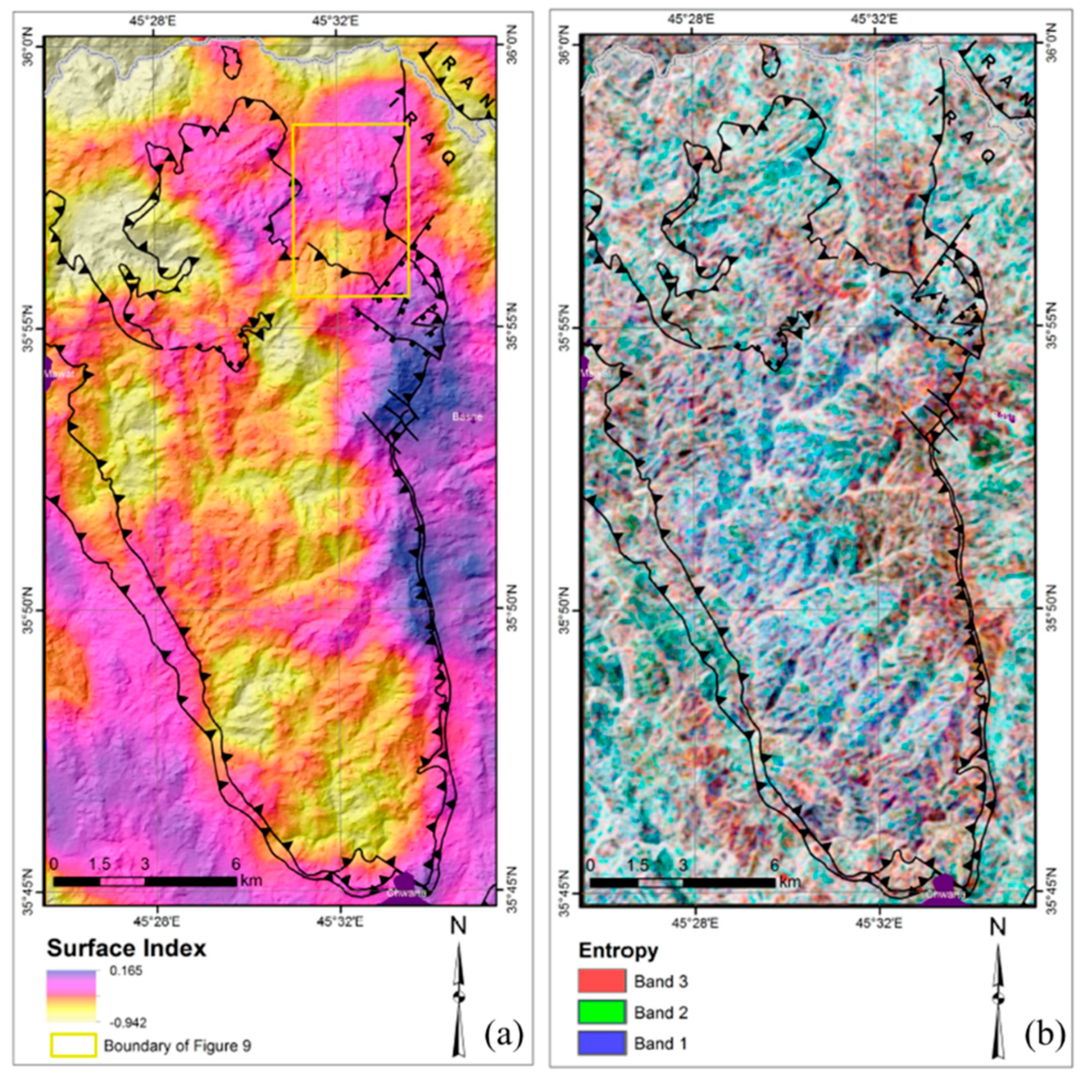
Figure 2.
Classification results for Liuyuan 1 using (a) Spectral angle mapping (SAM); (b) spectral information divergence (SID); (c) fully constrained linear spectral unmixing (FCLSU); (d) support vector machine (SVM); (e) random forest (RF); (f) neural network (NN); (g) 1-D CNN; (h) 2-D CNN; (i) 3-D CNN [124].
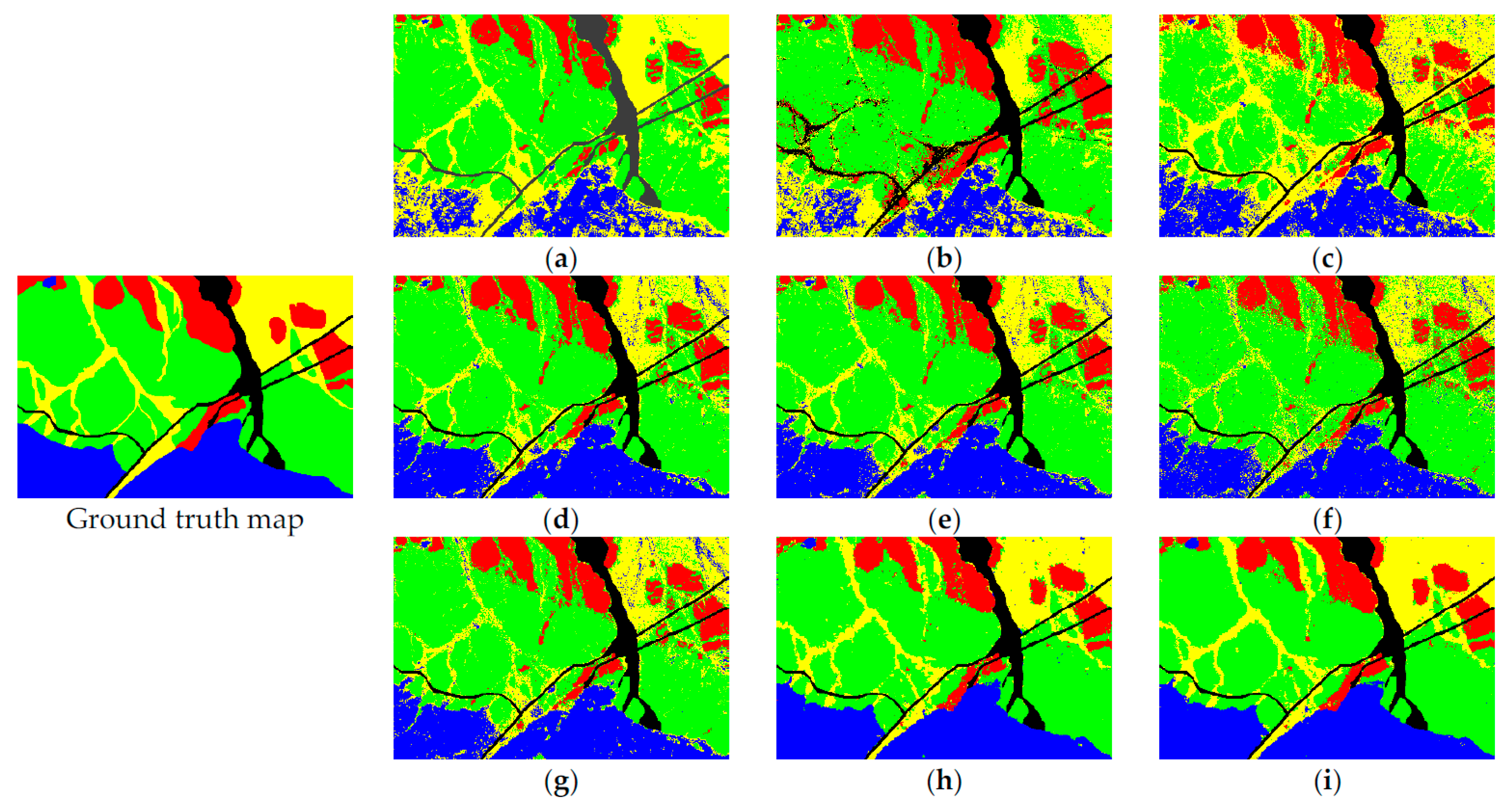
Figure 3.
(A) Thrust fault overlapping ASTER data (B) discriminated classes from combined derived from ASTER and DEM data [76].
Figure 3.
(A) Thrust fault overlapping ASTER data (B) discriminated classes from combined derived from ASTER and DEM data [76].
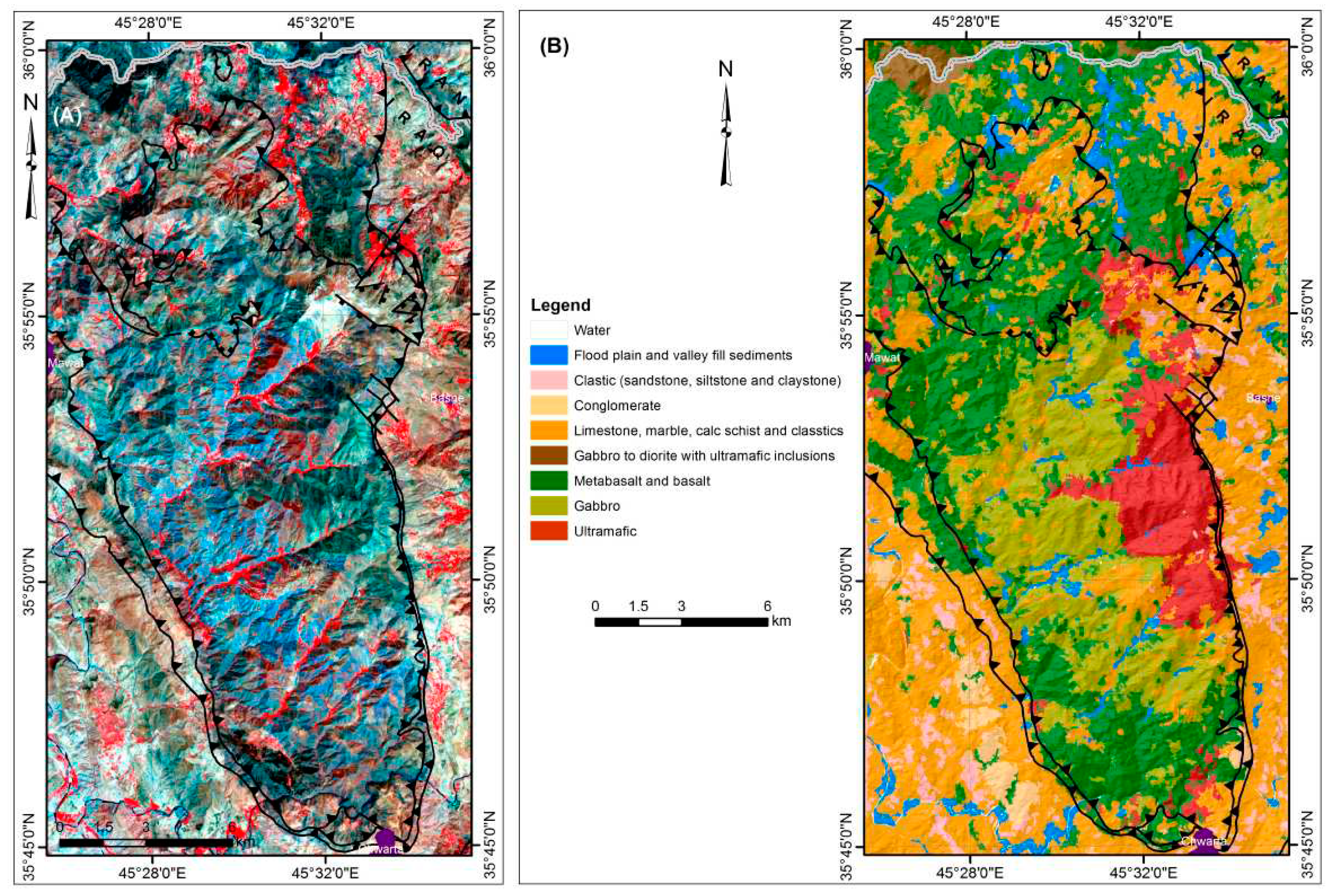
Figure 4.
Classification map obtained by (a) CNN based on fused ASTER, Sentinel-2A(S2A) and geochemical survey data, (b) RF based on fused ASTER, RF and geochemical survey data, (c) CNN based on ASTER and S2A, and (d) RF based on ASTER and S2A, modified form [23].
Figure 4.
Classification map obtained by (a) CNN based on fused ASTER, Sentinel-2A(S2A) and geochemical survey data, (b) RF based on fused ASTER, RF and geochemical survey data, (c) CNN based on ASTER and S2A, and (d) RF based on ASTER and S2A, modified form [23].
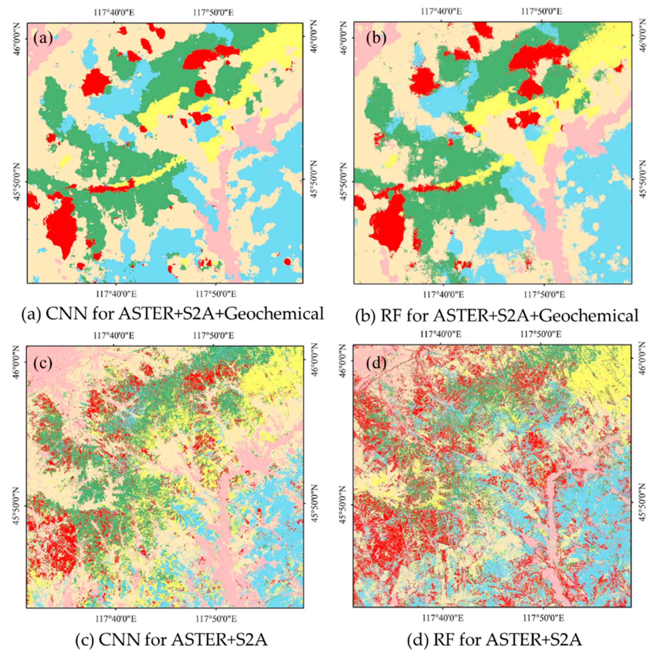
Figure 5.
(a) QuickBird image, and lithological maps generated using (b) the best spectral-only algorithm (ATM MNF SOM) and (c) the best integrated spectral–topographic algorithm (ATM-Li MNF SOM) [20].
Figure 5.
(a) QuickBird image, and lithological maps generated using (b) the best spectral-only algorithm (ATM MNF SOM) and (c) the best integrated spectral–topographic algorithm (ATM-Li MNF SOM) [20].
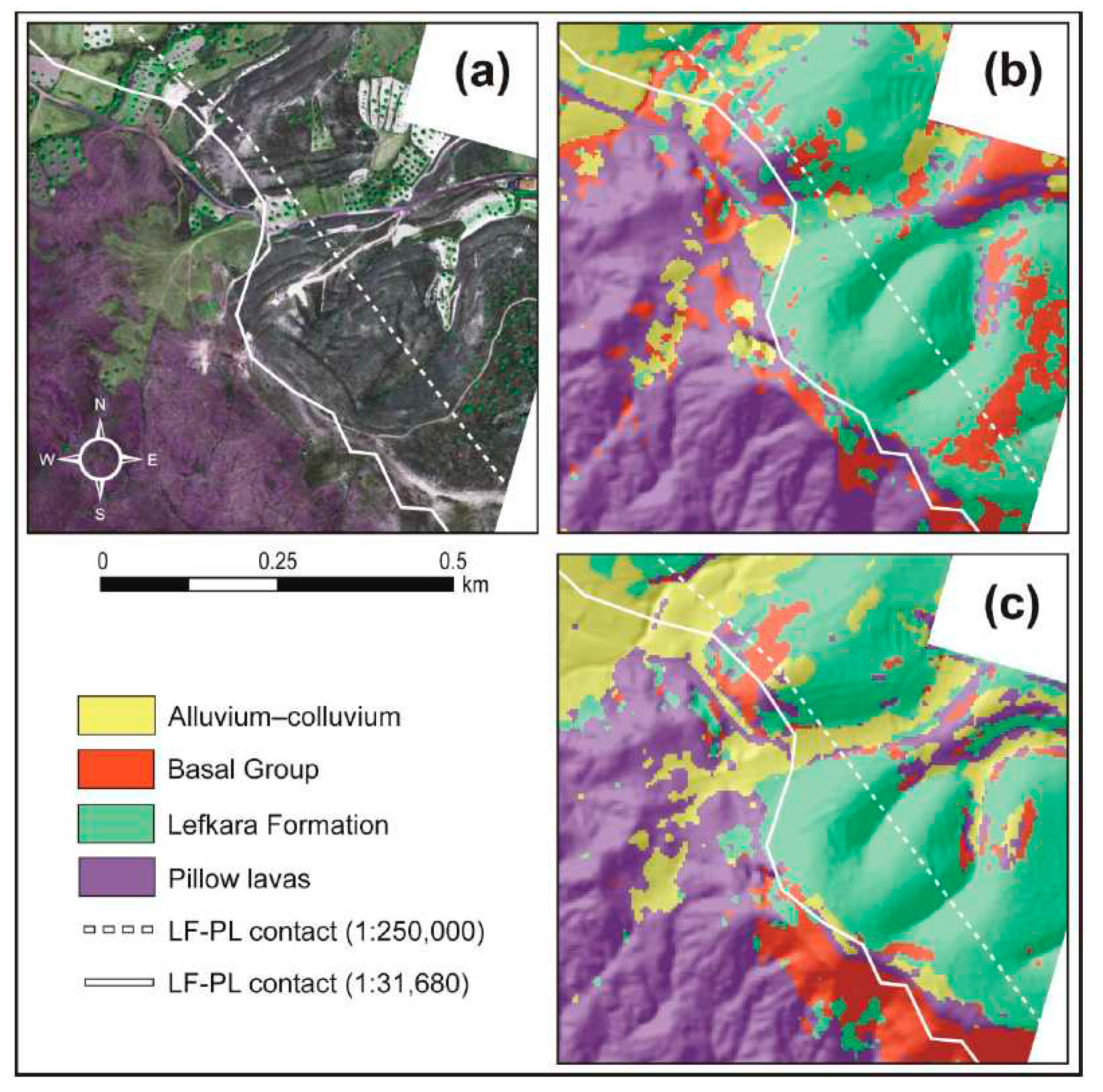
Figure 6.
The overall accuracy (A) and kappa (B) for different combination features with ML, SVM, and RF methods [96]. The figure illustrates the representation of various variables, where R denotes reflectance, BR signifies band ratio, TPI represents topographic position index, PCA stands for principal component analysis, and XY indicates spatial features.
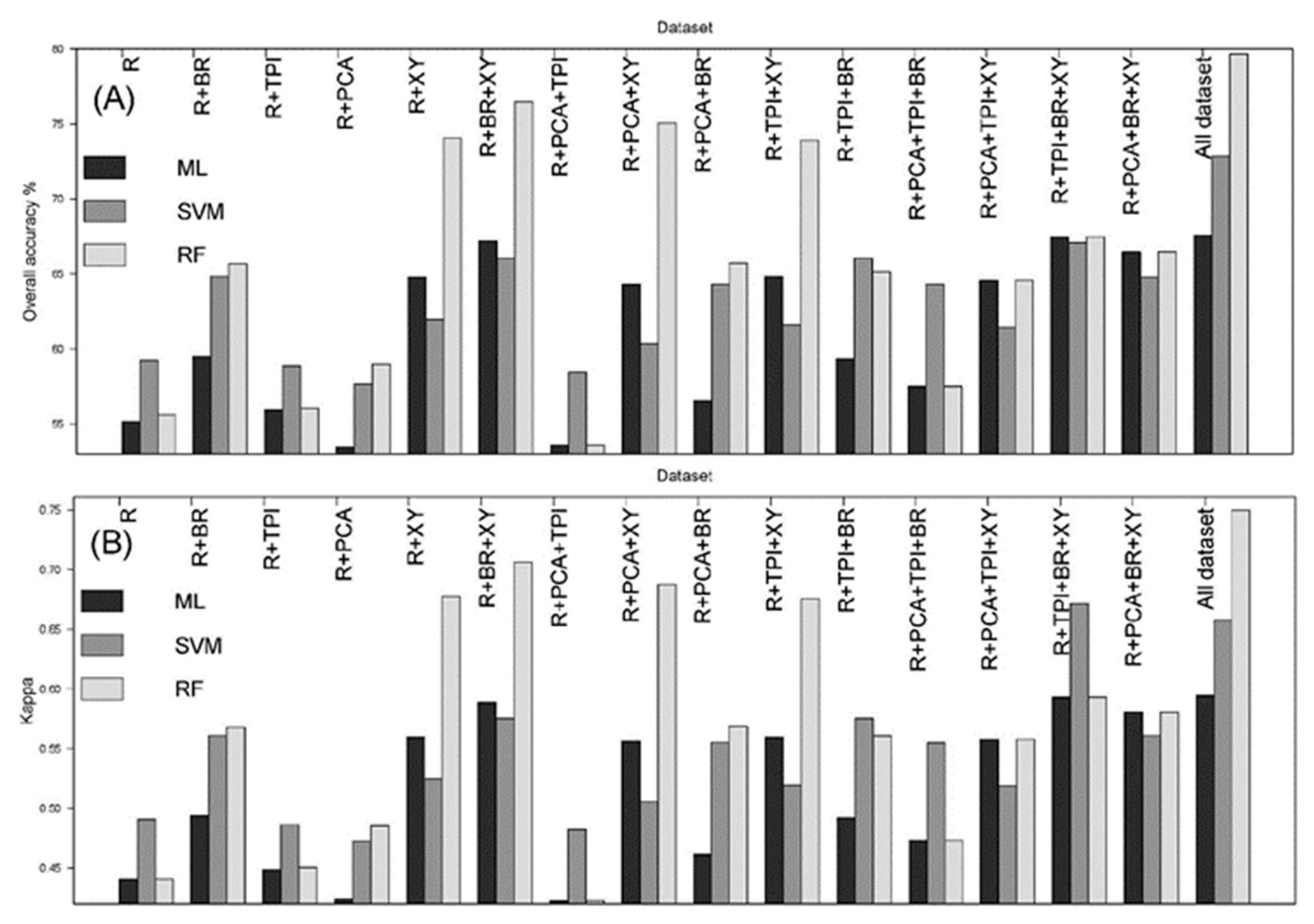
Figure 7.
(a)OLI image and (b)Lithological sketch of the study area, and lithological classification results of the study area based on (c) spectrum (SPEC), (d) fused SPEC and thermal (TEM), (e) fused SPEC, TEM and topographic (TOPO), and (f) SPEC, TEM, TOPO and textural (TEXT) [28].
Figure 7.
(a)OLI image and (b)Lithological sketch of the study area, and lithological classification results of the study area based on (c) spectrum (SPEC), (d) fused SPEC and thermal (TEM), (e) fused SPEC, TEM and topographic (TOPO), and (f) SPEC, TEM, TOPO and textural (TEXT) [28].
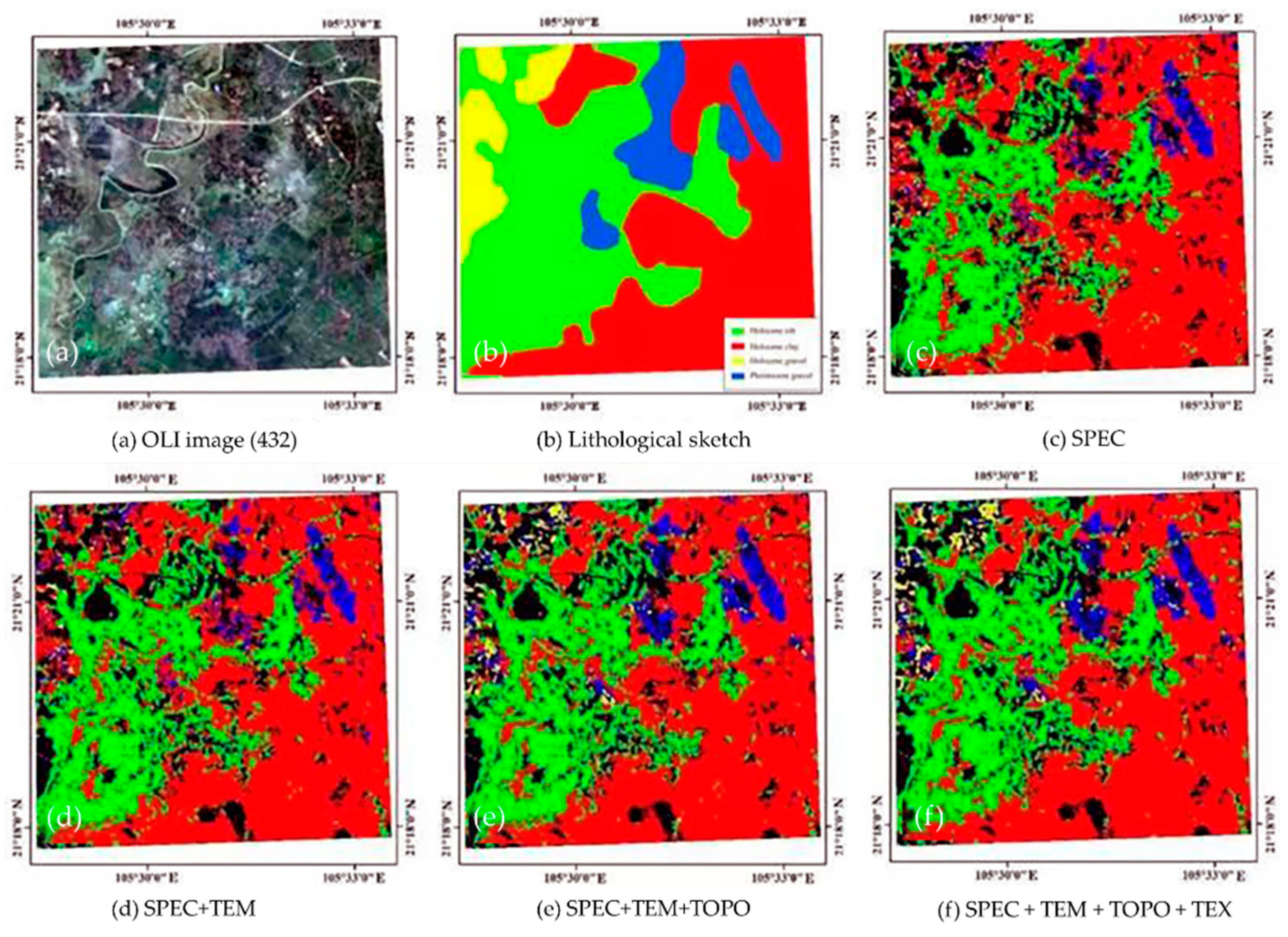
Figure 8.
Classification results of all the methods for Liuyuan 1. (a) SAM; (b) SID; (c) fully constrained linear spectral unmixing (FCLSU); (d) SVM; (e) RF; (f) NN; (g) 1-D CNN; (h) 2-D CNN; (i) 3-D CNN [124].
Figure 8.
Classification results of all the methods for Liuyuan 1. (a) SAM; (b) SID; (c) fully constrained linear spectral unmixing (FCLSU); (d) SVM; (e) RF; (f) NN; (g) 1-D CNN; (h) 2-D CNN; (i) 3-D CNN [124].
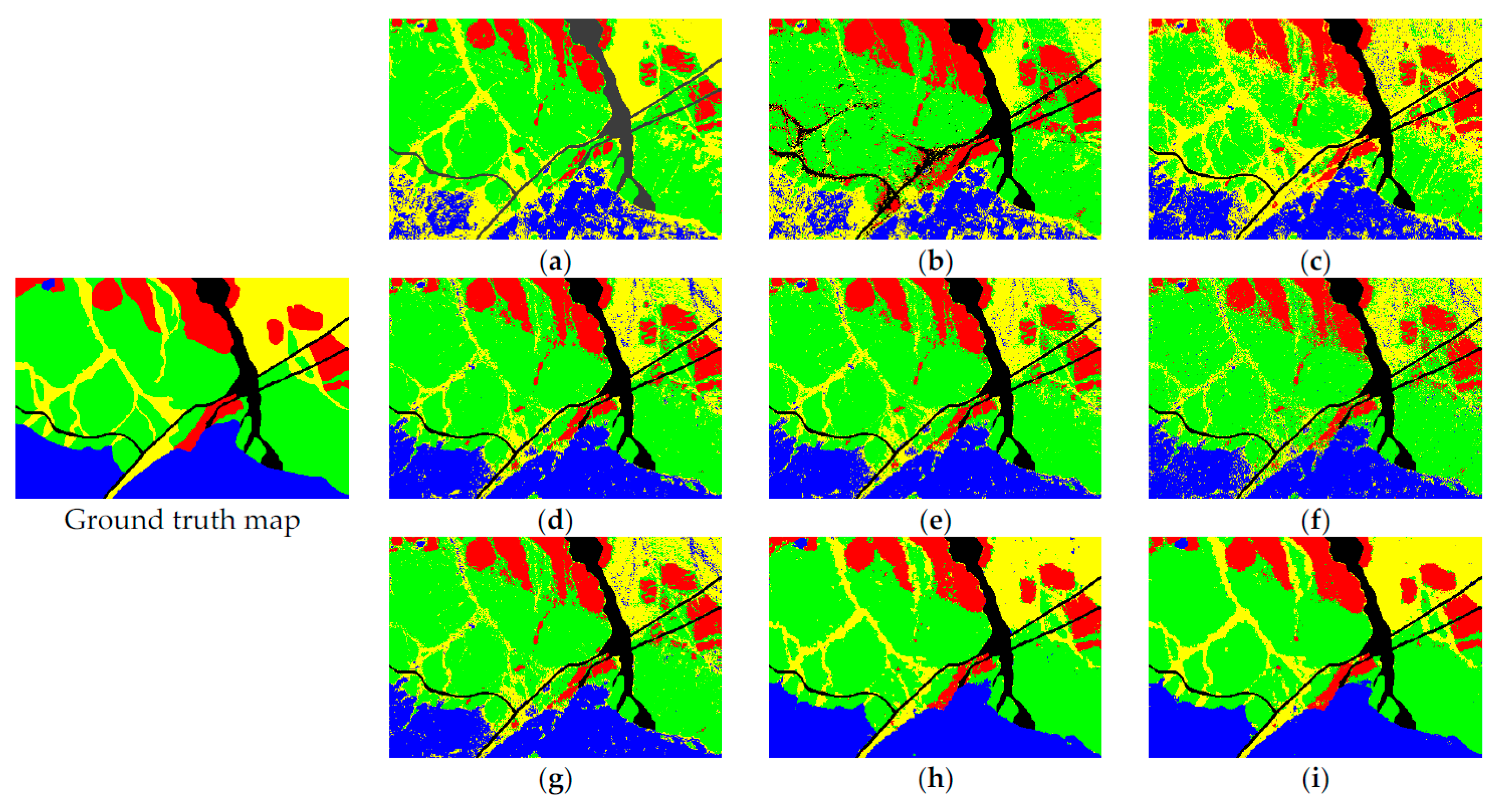
| ASTER | Radiometer | Resolution (m) |
Wavelength (µm) |
Wave-width (nm) | S/N |
|---|---|---|---|---|---|
| Band 1 | VNIR | 15 | 0.52–0.60 | 90 | ≥140% |
| Band 2 | 0.63–0.69 | 60 | ≥140% | ||
| Band 3 | 0.76–0.86 | 100 | ≥140% | ||
| Band 4 | SWIR | 30 | 1.60–1.70 | 92 | ≥140% |
| Band 5 | 2.145–2.185 | 35 | ≥54% | ||
| Band 6 | 2.185–2.225 | 40 | ≥54% | ||
| Band 7 | 2.235–2.285 | 47 | ≥54% | ||
| Band 8 | 2.295–2.365 | 70 | ≥70% | ||
| Band 9 | 2.360–2.430 | 68 | ≥54% | ||
| Band 10 | TIR | 90 | 8.125–8.475 | 344 | ≤0.3K |
| Band 11 | 8.475–8.825 | 347 | ≤0.3K | ||
| Band 12 | 8.925–9.275 | 361 | ≤0.3K | ||
| Band 13 | 10.25–10.95 | 667 | ≤0.3K | ||
| Band 14 | 10.95–11.65 | 593 | ≤0.3K |
| Sentinel 2 | Band | Wavelength(nm) | resolution(m) |
|---|---|---|---|
| Band 1 | Aerosols | 443.9nm (S2A) / 442.3nm (S2B) | 60 |
| Band 2 | Blue | 496.6nm (S2A) / 492.1nm (S2B) | 10 |
| Band 3 | Green | 560nm (S2A) / 559nm (S2B) | 10 |
| Band 4 | Red | 664.5nm (S2A) / 665nm (S2B) | 10 |
| Band 5 | Red edge 1 | 703.9nm (S2A) / 703.8nm (S2B) | 20 |
| Band 6 | Red edge 2 | 740.2nm (S2A) / 739.1nm (S2B) | 20 |
| Band 7 | Red edge 3 | 782.5nm (S2A) / 779.7nm (S2B) | 20 |
| Band 8 | NIR | 835.1nm (S2A) / 833nm (S2B) | 10 |
| Band 8A | Red edge 4 | 864.8nm (S2A) / 864nm (S2B) | 20 |
| Band 9 | Water vapor | 945nm (S2A) / 943.2nm (S2B) | 60 |
| Band 10 | Cirrus | 1373.5nm (S2A) / 1376.9nm (S2B) | 60 |
| Band 11 | SWIR 1 | 1613.7nm (S2A) / 1610.4nm (S2B) | 20 |
| Band 12 | SWIR 2 | 2202.4nm (S2A) / 2185.7nm (S2B) | 20 |
Table 4.
Satellite information of GF-1, GF-2, GF-3, GF-5 and ZY-3 independently launched by China. In the table, the following abbreviations are used: SR for Spatial Resolution, R for Revisit, OA for orbit altitude, and LT for launch time.
Table 4.
Satellite information of GF-1, GF-2, GF-3, GF-5 and ZY-3 independently launched by China. In the table, the following abbreviations are used: SR for Spatial Resolution, R for Revisit, OA for orbit altitude, and LT for launch time.
| Satellite | Band Range | SR (m) | R (day) | Swath(km) | OA | LT | reference |
|---|---|---|---|---|---|---|---|
| GF-1 | blue, green, red, MIR | 2/8 | 5 | 90/800 | 645km | 2013/4/26 | [40] |
| GF-2 | blue,green, red,NIR | 0.8/2 | 3-5 | 45/16 | 645km | 2014/8/19 | [86] |
| GF-3 | X, S, C, L | 1/3/8/25 | 1-4 | 30-40 | 755km | 2016/8/10 | [86] |
| GF-5 | VNIR,SWIR, MWIR | 30 | 16 | 60 | 705km | 2018/5/9 | [87] |
| HJ-1A CCD | VNIR | 30 | 700 | 2008/9/6 | [53] | ||
| ZY-1 02D | VNIR, SWIR | 30 | 55 | 60 | 705km | 2019/9/12 | [38] |
| ZY-3 | full-color, multi-spectral | 2.1/3.5/6 | 5/3 | 51/52 | 505km | 2012/1/9 | [88] |
Table 5.
The average overall accuracy (%) of cross-validation for classification accuracy assessment, modified from [16].
Table 5.
The average overall accuracy (%) of cross-validation for classification accuracy assessment, modified from [16].
| classifer | Hyperion | ASTER | Landsat 8 | Combined |
|---|---|---|---|---|
| MD | 49.02 | 66.82 | 63.55 | |
| SAM | 71.24 | 45.21 | 47.16 | |
| SID | 66.43 | 42.38 | 48.22 | |
| SVM | 87.03 | 64.89 | 60.79 | |
| MAXW | 71.98 | 54.21 | 60.78 | 70.80 |
| proposed | 91.93 | 75.90 | 67.16 | 93.22 |
Table 6.
Classification results for MLC and SOM classifiers, adapted from [20]. Li represents terrain features obtained from LiDAR data.
Table 6.
Classification results for MLC and SOM classifiers, adapted from [20]. Li represents terrain features obtained from LiDAR data.
| variable | MLC | SOM | |||
|---|---|---|---|---|---|
| OA(%) | Kappa | OA(%) | Kappa | ||
| ATM 9 | 61.6 | 0.50 | 60.3 | 0.48 | |
| ATM PCA | 51.4 | 0.37 | 50.2 | 0.35 | |
| ATM MNF | 59.3 | 0.46 | 65.5 | 0.54 | |
| ATM-Li | 61.9 | 0.50 | 70.2 | 0.60 | |
| ATM-Li MNF | 60.8 | 0.49 | 72.7 | 0.63 | |
Table 7.
Classification results of all the methods for Liuyuan 1. (a) SAM; (b) SID; (c) FCLSU; (d) SVM; (e) RF; (f) NN; (g)1-D CNN; (h) 2-D CNN; (i) 3-D CNN. Modified form [124].
Table 7.
Classification results of all the methods for Liuyuan 1. (a) SAM; (b) SID; (c) FCLSU; (d) SVM; (e) RF; (f) NN; (g)1-D CNN; (h) 2-D CNN; (i) 3-D CNN. Modified form [124].
| SAM | SID | FCLSU | SVM | RF | NN | 1D CNN | 2D CNN | 3D CNN | |
|---|---|---|---|---|---|---|---|---|---|
| OA | 75.87 | 72.12 | 73.42 | 84.68 | 86.01 | 81.27 | 84.38 | 94.18 | 94.70 |
| Kappa | 0.64 | 0.59 | 0.63 | 0.77 | 0.79 | 0.78 | 0.77 | 0.91 | 0.92 |
Disclaimer/Publisher’s Note: The statements, opinions and data contained in all publications are solely those of the individual author(s) and contributor(s) and not of MDPI and/or the editor(s). MDPI and/or the editor(s) disclaim responsibility for any injury to people or property resulting from any ideas, methods, instructions or products referred to in the content. |
© 2023 by the authors. Licensee MDPI, Basel, Switzerland. This article is an open access article distributed under the terms and conditions of the Creative Commons Attribution (CC BY) license (http://creativecommons.org/licenses/by/4.0/).
Copyright: This open access article is published under a Creative Commons CC BY 4.0 license, which permit the free download, distribution, and reuse, provided that the author and preprint are cited in any reuse.


