
Submitted:
21 July 2023
Posted:
25 July 2023
You are already at the latest version
Abstract
A close-range photogrammetric approach and its implementation using a CNC device and a macro camera are proposed. A tailored image acquisition approach is proposed that is implemented using this device. To increase reconstruction robustness and accuracy, the key point features detected in the acquired images are tracked across multiple views from multiple viewpoints at multiple distances. This approach reduces spurious correspondences and, as a result, the estimation accuracy of calibration parameters is increased and reconstruction errors are reduced. Qualitative and quantitative evaluation demonstrate the efficacy and accuracy of the proposed approach, which exhibits micrometre resolution and low implementation cost.
Keywords:
surface scanner
; photogrammetry
; close-range photogrammetry
; feature tracks
1. Introduction
This work regards an approach to the measurement of the physical characteristics and features of scanned surfaces. The primary goal is to accurately digitise the variations in elevation, shape, and texture of surfaces in high detail, in the spatial scale micrometres. The secondary goal is to achieve this digitisation in a cost-efficient manner and with simple technical means so that the result is widely applicable. Motivation stems from the detailed digitisation of surfaces for a multitude of purposes, such as the documentation of cultural heritage artefacts, the creation of realistic textures for digital design, industrial production control, or the facilitation of research for the understanding of tactile sensation.
Several approaches achieve accurate and reliable surface digitisation in large detail. Computed tomography uses X-rays to provide volumetric scans of objects and their surfaces and has been used for the digitisation of small objects [1]. Magnetic resonance tomography provides volumetric scans and has been also used for small objects [2]. Laser scanning uses the time-of-flight principle to measure distances and reconstruct surfaces but is not manoeuvrable or versatile. Structured light scanners project light patterns onto surfaces, capture the deformed patterns using a camera and, from these deformations, estimate surface structure.
Albeit highly accurate, tomographic methods exhibit severe costs and can be applied only in specialised laboratories. Compared to laser scanning and structured light scanning, photogrammetry can be marginally less accurate, but requires less specialized equipment. Photogrammetry relies on standard cameras, which are more affordable and widely available and, thus, is a more cost-effective solution. Moreover, photogrammetry captures the visual appearance of surfaces, producing high-resolution and highly detailed textured models that accurately represent visual appearance. Compared to laser and structured light methods, photogrammetry is passive, in that it does require the projection of energy in the form of radiation (e.g., light, X-rays, etc.) upon the scanned surface. This is important in light-sensitive materials, encountered in historical, archaeological, biological, and cultural contexts.
This work employs the contactless, flatbed photogrammetric scanner from [3] which was developed for the creation of 2D image mosaics of surfaces in the micrometre range. This scanner is comprised of off-the-shelf as well as printable components, which can be found in [3]. It costs less than , offers resolution and has a scanning area of . In this work, this hardware is used to acquire 2.5D surface reconstructions.
We refer to the digitisation of surfaces as 2.5D digitisation. This is different from representing surface structure using an elevation map. In 2.5D digitisation, the surface reconstruction is comprised of a mesh of textured triangles, as in the 3D digitisation of objects.
2. Related work
The literature is first reviewed in terms of the applications where close-range photogrammetric systems are employed, as well as the optics and illumination methods utilised for their implementation. Thereafter, data acquisition quantities and reconstruction methods are reviewed. Last but not least, photogrammetry creates reconstructions “up to scale”, that is, the resultant reconstruction is not in metric units but in arbitrary ones. As the goals of this work include surface measurement, the ways that the scale factor is estimated for close-range photogrammetric methods conclude this section.
2.1. Applications
Photogrammetry has been applied in a wide variety of contexts over the last three decades, mainly referring to large-scale reconstruction targets in the range of hundreds to a few meters, such as built and terrain structures captured from aerial views, indoor environments, and cultural heritage objects. More recently, close-range photogrammetry has found applications in the high-resolution reconstruction of structures of much smaller scale, of industrial [4,5,6], biological [7], archaeological [8,9], anthropological [10], and cultural interest [11,12], in the range of millimetres (see [13] for a comprehensive review of close-range photogrammetry applications).
2.2. Motorisation
When using a single camera, the motion of the camera relative to the subject is required to obtain 3D information. Motorisation of camera movement has been used in photogrammetric reconstruction. The main strategies of motion are either circular around the target, using a turntable, or in a Cartesian lattice of viewpoints [14]. Cartesian approaches exhibit the advantages of being unconstrained of the turntable size, as well as that the camera can be moved arbitrarily close to the scanning target. This work follows the latter approach so that it can scan wider surfaces and avoid the occurrence of shadows and illumination artefacts. The most relevant scanning apparatus to this work is [15], which uses a CNC to move the camera.
2.3. Optics
For objects in the millimetre and sub-millimetre range, zoom and microscopic, or “tube”, lenses have been used [14,16,17], employing tedious calibration procedures and relatively inaccurate results [18]. Instead, macro lenses are much more widely used in the photogrammetric reconstruction of very small structures [19]. However, macro lenses exhibit a very limited depth of field. This limitation makes photographs acquired with a macro lens to be partially out of focus. The depth of field of macro lenses is usually so small that when imaging a planar surface its centre is focused but the periphery of the image is blurred1. To compensate for this effect, focus stacking [20] is employed in macro photography [21].
2.4. Illumination
Illumination is necessary for photogrammetric methods so that the surfaces to be reconstructed are visible to the camera sensor. Photogrammetry typically operates upon environmental illumination. Ambient illumination is ideal for photogrammetric methods because it prevents the formation of shadows, which confound the visual documentation of the reconstructed surfaces. Most works use setups that insulate the target object from environmental illumination and use a specific light source in conjunction with illumination diffusers, which prevent the formation of shadows. In closer relation to this work, some systems use light sources that move along with the camera [22,23,24].
Purposefully designed illumination is used in photogrammetric methods to facilitate the establishment of more stereo correspondences. This technique is known as “active illumination”, “active photogrammetry”, or “structured light” [23,25,26]. Pertinent methods use active illumination to support the reconstruction of the geometry of the reconstructed surface, by artificially creating reference points on the surface which can be matched across images. The disadvantage is that the projected light alters the visual appearance of the reconstructed surfaces. As such, this work does not use active illumination as it strives to realistically capture the visual appearance of the target surfaces.
2.5. Data
The data acquired from the close-range photogrammetric methods vary depending on the hardware and optical apparatus employed.
Works that report scanning areas fall in the range of . Specifically, the maximum area reported from these works is (approximately) as follows: [16], [25], [23], [9], [27], [15], [22], [28], [8], [17], [16], and [28]. Out of these works, only [16] reports the achieved resolution, which is .
Works that report the number of images and pixels processed fall in the range of . The data load is calculated as the number of utilised images times the resolution of each image. Specifically, the maximum number of pixels reported from these works is (approximately), in , as follows: =9.6 [17], [24], [27], [26], [15], [9], [7], and [22].
2.6. Reconstruction
Several works use commercial photogrammetry software to reconstruct the imaged scene, with the most popular being the Pix4D and AgiSoft suites. As discussed in Section 4.3, these software suites provide less accurate results, as they are agnostic to the image acquisition strategy employed in this work and do not utilise feature tracking.
Some of the reviewed works perform partial reconstructions which result in individual point clouds and then merge them using point cloud registration methods. These methods are mainly based on the ICP algorithm [29,30], either implemented by the authors or provided by software utilities, such as CloudCompare and MeshLab. The disadvantages of merging partial reconstructions are the error of the registration algorithm and the duplication of surface points that are reconstructed by more than one view. These disadvantages impact the accuracy and efficacy of the reconstruction result, respectively.
2.7. Scale
Several ways to generate metric reconstructions have been proposed. One way is to place markers at known distances so that when they are reconstructed they yield estimates of the absolute scale. However, this method is prone to the localisation accuracy of said markers. An improvement to this approach comes from [24] which uses the ratio of the reconstructed objects over their actual size, which is manually measured. In addition, it requires the careful selection of the reference points to estimate the size of the object both in the real and the reconstructed objects and is, thus, prone to human error. This can be a difficult task for free-form artworks as they may not exhibit well-defined reference points (i.e., as opposed to industrially manufactured objects). Therefore, the accuracy of this approach is dependent on the accuracy of manual measurements and the measurement of the size of the reconstruction which is also manual, as it is performed in a 3D viewer.
Another way is to include objects of known size in the reconstructed scene, such as 2D or 3D markers of known size [22,24,27]. This method does not involve human interaction and is not related to the structure of the reconstructed objects. The main disadvantage of this approach is the production of these markers, as printing markers at this small scale is not achievable at this fine scale by off-the-shelf 2D or 3D printers.
Finally, a way to estimate the scale factor is based solely on the reprojection error of the correspondences of a stereo pair [31]. This approach is independent of the shape of the target object and does not require human interaction. However, this approach is formulated for a stereo pair and not for a single camera and, also, is highly dependent on the calibration accuracy of this pair.
2.8. This work
This work puts forward a photogrammetric approach that is powered by a motorised apparatus, implemented by a modest computer and a conventional CNC device.
The photogrammetric approach is characterised by two novel characteristics. First, a tailored image acquisition is implemented using said apparatus that acquired images of the target surface at multiple distances. Second, key point features are tracked across multiple views from multiple viewpoints and at multiple distances, instead of only being corresponded in neighbouring images. These characteristics increase reconstruction robustness and accuracy.
The motorised apparatus has been proposed in [3] for the acquisition of 2D surface mosaics, in micrometre scale. It is reused in this work, to obtain 2.5D surface digitisations. The Cartesian nature of this apparatus facilitates the image acquisition process and enables more practical digitisation of surfaces than a turntable. In addition, the ability to move the camera and source of illumination very close to the target surface reduces illumination artefacts and shadows. Finally, the apparatus can be easily assembled and the total cost of all its components, including the camera, sums below (see [3]).
3. Method
The proposed approach combines two elements that increase its robustness against reconstruction errors, due to spurious correspondences. The first element is the way of image acquisition. Specifically, besides the necessary images required to cover the target surface at a close distance, additional images are acquired at larger distances. These images are fewer and overview the same areas that are imaged at closer distances. The second is the tracking of features across images. When combined, these elements aid the reduction of spurious correspondences. As a result, the estimation accuracy of calibration parameters is increased and reconstruction errors are reduced.
3.1. Data acquisition
Initially, the camera is calibrated to estimate its intrinsic parameters and its lens distortion. The FoV of the camera is also estimated through this calibration.
Images are acquired in layers across the distance, or elevation, from the scanned surface. The locations of image acquisition form a hypothetical square frustum above the scanned surface. In each layer, camera locations form a hypothetical grid. Within each layer, the image acquisition locations are set so that horizontally and vertically neighbouring images of that layer exhibit significant overlap; the percentage of this overlap is denoted as . Across consecutive layers, image acquisition locations are aligned so that the medial overlap across neighbouring images is maximised. The amount of medial overlap is determined by the distance of consecutive layers. The purpose of wide overlap is the maximisation of correspondences to increase the number of point correspondences in stereo pairs.
Using the FoV estimate and the intended amount of lateral overlap, the camera locations are pre-computed for each layer. Each layer doubles the elevation from its previous so that an image of a higher layer medially overlaps with 4 images from a lower layer. Camera locations are saved in a file, which is called the “scan plan”. These locations are then converted to scanner coordinates and a corresponding segment of G-code2 is generated. This code is transmitted to the CNC and images are acquired, using the software interface from [3]. The image filenames are associated with the camera locations in the scan plan. To reduce scanning time and mechanical drift, each layer is scanned in boustrophedon order.
The acquired images are not compensated for lens distortion at this stage. Due to the focused stacking operation that is applied individually on each image, lens distortion is also individually estimated at a later stage (see Section 3.3.2).
3.2. Feature detection and tracking
Key point features with content descriptions are detected in all images. In the implementation, SIFT [32] features are employed, however, any other type of key point features can be used.
3.2.1. Image pairs
The pairs of neighbouring images, let and , within and across layers are found from the scan plan. Correspondences are then established across laterally and medially neighbouring images, as follows.
First, the cascade hashing method in [33] is employed to accelerate and robustify feature matching. The hashing is guided from the content descriptors of the detected key points to consider only similar key points in the matching task.
Second, to filter erroneous correspondences a symmetrical, or left-to-right check [34] is employed. In other words, to establish a feature correspondence, we require that the same key point feature pair is found both when features of are matched against and vice versa. Conventionally, to avoid doubling the computational cost, when establishing matches in one direction key point similarities could be recorded and utilized when scanning in the opposite order. Unfortunately, our GPU RAM is not sufficient to record this information, for large targets. Thus, {,} and {,} are treated independently and the doubling of computational cost is not avoided. If a GPU with larger memory would be available the aforementioned method could be employed to halve the computational cost of this task.
Third, the fundamental matrix, F, is estimated from the available correspondences at this stage. This estimate is obtained using RANSAC [35] to reject erroneous correspondences, or “outliers”. The remaining, “inlier”, correspondences are used to estimate F, using least squares. The estimated matrix is used to constrain the search for correspondences along a line rather than the entire image. Correspondences are approved only if the reprojection error is below threshold . Otherwise, they are discarded. In this way, a matrix F is computed for each of the image pairs.
Theoretically, F could be calculated for each image pair using the intrinsic parameters of the camera and the relative poses of camera pairs from the scan plan instead of the aforementioned procedure. In practice, however, we found that the small, mechanical inaccuracies of the CNC lead to erroneous F estimates. The resulting error is large enough to cast the calculated F overly inaccurate for outlier elimination and the above-mentioned task necessary.
3.2.2. Feature tracks
To increase robustness, features are tracked across images, as follows. Let a physical point in the scene that was detected and corresponded in three images or, otherwise, two image pairs. The images of these pairs can be laterally or medially neighbouring. These two correspondences associate the same feature in the three images and comprise a “feature track”. We keep tracks comprised of three or more features.
These tracks are used to further reject feature matches, using the fundamental matrices computed for the image pairs of these matches. Using the epipolar constraint, the position of each feature in the track is checked to determine its consistency with the fundamental matrix of every pair. This check is implemented using the “chain” of fundamental matrices that are associated with the images in which each feature is tracked. The check projects a feature from the first image of a track to the last image of this track. If this projection occurs at a distance greater than then the track and all corresponding feature matches are rejected.
Feature tracks are not constrained in laterally neighbouring images, but are also established using correspondences across layers as well. This is central to achieving overall consistency in surface reconstruction. The reason is that the spatial arrangement of features in images of greater distance to the surface constrains the potential correspondences in images at closer distances. Through this constraint, erroneous correspondences are reduced.
The memory requirements for the succeeding tasks depend on the number of tracked features found. Depending on the number of input images the requirements for memory capacity may be large. It is possible to reduce memory capacity requirements at this stage, by discarding some of the feature tracks. If this is required, then it is recommended to discard the tracks with the fewest features. The reason is that they carry less information and they are, typically, much larger in number.
3.3. Reconstruction
The surface of the object is reconstructed as a textured mesh of triangles. This mesh is comprised of two lists. The first is a list of 3D, floating point locations that represent the mesh nodes. The second is a list of integer triplets that contain indices to the first list and indicate the formation of triangles through the represented nodes. A texture image accompanies the mesh, along with a third list of 2D coordinates that represents the texture coordinates of each node; thus the third list has the same length as the first one.
3.3.1. Initialisation
Using the feature tracks as a connectivity relation, a connected component labelling of the input images is performed. After this operation, the largest connected component is selected. The rest of the images, which belong to smaller components, are discarded. The discarded components correspond to groups of images that are not linked, through fundamental matrices, to the rest. As such, they cannot contribute to the main reconstruction. They are discarded to reduce memory capacity requirements.
The reconstruction method requires an image pair as the basis for the surface reconstruction. This pair is selected to exhibit a wide baseline to reduce reconstruction uncertainty and error [36]. The reason is that a wider baseline results in more separation between the optical rays, allowing for more accurate triangulation and reducing ambiguity in the 3D reconstruction. At the same time, the reliability of this pair depends on the number of features/correspondences existing in this pair. Thus, the initial pair is selected as the one that maximizes the product of the baseline with the number of correspondences.
3.3.2. Sparse reconstruction
A sparse reconstruction is first performed, using the camera poses of the scan plan, as initial estimates. The purpose of this reconstruction is to refine these poses from the images and the estimated intrinsic camera parameters.
The OpenMVG [37] is utilised for this purpose and the resultant reconstruction is the camera poses and a sparse point cloud. In this context, the Incremental Structure from Motion pipeline [38] is followed.
Finally, a bundle adjustment step, using [39], is performed, based on the scan plan. This final step is adapted to optimise only the lens distortion parameters for each image. The reason is that the intrinsic and extrinsic camera parameters have been already refined from the previous operation. Lens distortion parameters are not defined in the previous step. The reason is that they change from image to image due to the effect of the focused stacking operation that takes place on the camera hardware.
The method is formulated in Algorithm 1.
| Algorithm 1:Incremental Structure from Motion |
|
3.3.3. Dense reconstruction
A mesh of triangles is computed based on the input, sparse point cloud. The input is the images, camera poses, and sparse reconstruction from Section 3.3.2.
The computation generates a depth map for each image. Using the depth maps of neighbouring images dense point cloud is generated. Implementation is based on [40]. Following [41], a mesh surface that best explains the dense point cloud is generated. Afterwards, this mesh is refined via the variational method in [42].
Despite the high accuracy of the utilised methods, both the mesh and the camera poses are not infallible, thereby containing some amount of error. These inaccuracies tend to be pronounced more in the texture of the output mesh, particularly when a large number of images is utilised. To cope with these inaccuracies in the generation of the output mesh, the approach in [43].
In the implementation, the OpenMVS [44] library is utilised.
3.4. Output
The resultant reconstruction is a textured mesh of triangles. This result is comprised of a data structure that encodes the locations of these triangles in space.
The texture map is computed from the input images as follows. During this computation, a data structure is generated. This data structure has the same dimensions as the texture map and stores one integer per pixel. The value of each pixel encodes the id of the mesh triangle textured by that pixel.
In addition, two images are also computed from the above outputs, both using the Z-buffering method [45]. The first is a depth map, that encodes the elevation of the area encoded in each pixel. The second is an orthoimage, or otherwise a rectified image in which perspective distortions have been removed. Both images have a uniform scale and, thus, can be used as maps where the imaged structures can be directly measured. These images are generated as follows.
When computing the depth map the id of the mesh triangle that appears on each pixel is stored in an additional image that keeps this id for each pixel of the depth map. Moreover, for each depth map pixel, a location inside the triangle mesh is computed, as the intersection of the perpendicular line from that pixel with the mesh triangle. The barycentric coordinates of the intersection point inside the triangle are then calculated. The triangle id is used to look up the corresponding triangle in the texture map. The barycentric coordinates are used to find the point inside the texture map triangle. As this point may not have integer coordinates, bilinear interpolation is utilised to acquire the final colour value.
The result is stored in PLY format3, in two files. The first file contains the mesh representation and uses the binary representation of the format to save disk space. The second file contains the texture, in JPEG or PNG image file format.
4. Results
Materials and methods used for the implementation of the proposed approach are reported, followed by experimental results. These results are qualitative and quantitative. Qualitative results report the applicability of the proposed approach compared to conventional photogrammetric methods. Quantitative results measure the computational performance and the accuracy of surface reconstruction. All of the surface reconstructions shown in this section are provided as supplementary material to this paper.
4.1. Materials and data
The same computer was used in all experiments. Its specifications were as follows: CPU x64 Intel i7 8-core , RAM , GPU Nvidia RTX RAM (RTX2060 SUPER), SSD , HDD . The critical parameter is CPU and GPU RAM as they determine the number of correspondences that can be processed and, therefore, the area that can be reconstructed. The implementation of the scanning device is described in detail in [3] along with information for its reproduction through a CNC printer.
The visual sensor was an Olympus Tough TG-5, with a minimum focus distance of , a depth of focus of , a revolution of , and a FoV of . The depth of focus is currently the limit of the surface elevation variability that the proposed system can digitise. To store the data an SD card is utilised. The storage capacity of this card determines the maximum number of images that the system can acquire.
The maximum elevation of the CNC was . This elevation determines the height of a hypothetical square frustum. When the sensor is at that elevation level, it occurs at its top. The doubling of the elevation for each layer is to create a medial overlap of . In this way, an image at a higher layer oversees 4 images from a lower layer. The number of layers was 4, and they were configured as noted in Table 1. In this table, E is the elevation, n is the total number of acquired images, while and are the numbers of images acquired in the horizontal and vertical dimensions, respectively. Moreover, and are the lengths of the steps that the camera is moved to acquire an image in the horizontal and vertical dimensions, respectively. Finally, is the length of the side of the square surface region that is imaged by an image pixel, at the specific layer.
In all experiments, illumination was produced by the sensor’s flash. The flash moves along with the camera, as in [22,23,24] (see Section 2.4). In this work, a ring flash is employed which is a circular illumination device that fits around the camera lens, creating a ring of light around the subject. Ring flashes provide even and shadow-free illumination for close-up shots of small subjects and evenly light the subject from all angles.
Sensor brightness, contrast, and colour balance were set to automatic. The utilised sensor provides images encoded in JPEG format. The average size of the image file is . Image acquisition and image file retrieval details, as well as CNC control, are provided in [3]. Focused stacking was implemented by the sensor hardware and firmware.
4.2. Reconstruction area and scale
In general, Cartesian camera motion is not restricted by the turntable configuration. That is, given a large enough CNC an arbitrary area can be scanned. The limitation of this work regarding the scanning area is the memory capacity of the utilised computer. Using the computational means available (see Section 4.1) the maximum scanning area achieved is , which is wider than the approaches presented in Section 4.2 that present results in the range of . It is nevertheless stressed that the proposed approach does not require stitching of partial results, which is a source of additional error.
For the reconstruction of a surface area, 3456 images were acquired whose dimension was . These images occupied on the hard drive of the computer. In these images, million key point features were detected. The computation took and the amounts of RAM utilised were and for the CPU and the GPU, respectively. The result was comprised of a mesh with 284558 nodes and 568076 triangles and a texture map of .
In contrast to the methods cited in Section 2.7, this work bases the scale factor estimation on the extrinsic parameters of the camera. Specifically, initial estimates of camera locations are obtained from the scan plan. This accuracy is relatively high and based on the accurate motorisation of CNC devices. Nevertheless, this accuracy is further refined by the bundle adjustment step of Section 3.3.2.
For the surface reconstructions, in all experiments, the following parameter values were utilised: , , and .
4.3. Qualitative
The purpose of this qualitative experiment is twofold. First, to investigate the overall accuracy of the proposed approach. Second, to test its applicability in challenging reconstruction targets in terms of reconstruction appearance when challenging materials are digitised.
4.3.1. Accuracy
When performing photogrammetry with large numbers of images, i.e., hundreds or thousands, camera localisation errors accumulate, resulting in reconstruction inaccuracies. In this work, this problem is reduced due to the establishment of feature tracks, particularly, across multiple distances. The underlying idea is that images at larger distances anchor the accumulation of error, while images at closer distances are employed for the reconstruction of details. Images at intermediate distances facilitate correspondence establishment across distances.
To illustrate this point, the following experiment uses the same images, as acquired by the proposed method in two conditions. In the first condition, the proposed method is utilised. In the second condition, the Pix4D photogrammetric suite was employed. Although the input images are the same, the conventional photogrammetric method employed in the second condition does not actively search for feature tracks.
The reconstruction target a handcrafted engraving at the handle of a silver spoon, which occupies an area of . In Figure 1, indicative original images and the obtained reconstructions are shown. The first row of Figure 1 shows one image from each layer, pertinent to the first experimental condition. In the second condition, the images were acquired from the distance shown in the rightmost image of this row.
The middle and bottom rows Figure 1 show reconstruction results, in the following way. The left column shows the textured reconstruction and the rest only its geometrical structure. The second from the left column shows the reconstruction frontally. The second from the right column shows the reconstruction rotated by and the right column by . The middle row shows the reconstruction result for the first condition and the bottom row for the second.
It is observed that the proposed method yields more accurate structure reconstruction both locally and globally. Local accuracy improvements are observed in the reconstruction of the hand-carved spoon structure. In the first condition, these structures are more accurately reconstructed, while the second condition exhibits higher noise levels than the proposed approach. Global accuracy improvements are observed in the side views of the reconstructed surface, as in the second condition the surface appears spuriously curved. Both improvements are attributed to the effect of feature tracks and their contribution to better camera localisation, which leads to more accurate reconstruction.
4.3.2. Appearance
Stereo vision and photogrammetry are usually incapable of reconstructing shiny surfaces. The reason is that such surfaces reflect different parts of the environment from each viewpoint and thereby the “uniqueness constraint” [46] is not met, leading to reconstruction errors.
This phenomenon is evident in images from the top layers, in Figure 1, as well as in Figure 2 and Figure 5 below. However, at very close distances, i.e., from the bottom layer, specular reflections are suppressed. The reason is that the imaging sensor and the light source are so close that the specularities occur outside the sensor’s FoV. Moreover, due to the ring configuration of the illumination source, the presence of shadows is minimal.
In this work, the images from the lowest layer are used to texture the reconstructions because they contain the largest number of pixels per unit area of the imaged surface. Due to the aforementioned phenomenon, they are also devoid of shadows and illumination specularities. This is to our advantage for two reasons. First, the reconstructed model can be re-lighted when used in a virtual 3D environment. Second, its material type can be defined in graphical rendering. This way, illumination specularities and shadows can be realistically simulated depending on the virtual viewpoint and the virtual source of light.
4.4. Quantitative
To measure the accuracy of reconstruction targets of known size and structural features are utilised. Such targets are coins, as well as metallic nuts and screws. The purpose of the experiment was to measure their reconstructed dimensions and compare them with the true ones.
4.4.1. Coins
Circular coins were scanned. The scanned coins belong to the Euro currency. All eight coins from this family were scanned. The true dimensions are known by the manufacturer and are public knowledge. These dimensions, the measured dimensions and the percentage of measurement error are reported in Table 2. Original images are shown in Figure 2 in the following order: top row first and, in each row, the order is from left to right. The corresponding reconstructions are shown, in the same order, in Figure 3.
Furthermore, to assess distortions in the reconstruction, we used the orthoimages images of the coin reconstructions. Specifically, the depth map from a frontal view was computed using Z-buffering [45]. Canny edge detection [47] was performed in that map, detecting depth discontinuities. Circles were robustly detected using RANSAC to eliminate outlier edges. The inlier edges were used to fit circles, using least squares. In Table 3, deviations of the detected edges from the fitted circle are reported, as the mean distance (and standard deviation) of these edges from the fitted circle. In Figure 4, shown are the employed depth edges superimposed on the orthoimages of the textured reconstructions.
4.4.2. Nuts and screws
Metallic nuts and screws were scanned in a second experiment for reconstruction accuracy. Original images are shown in Figure 5 and their reconstructions are shown, in the same order, in Figure 6. The ground truth dimensions of these items were measured using a calliper.
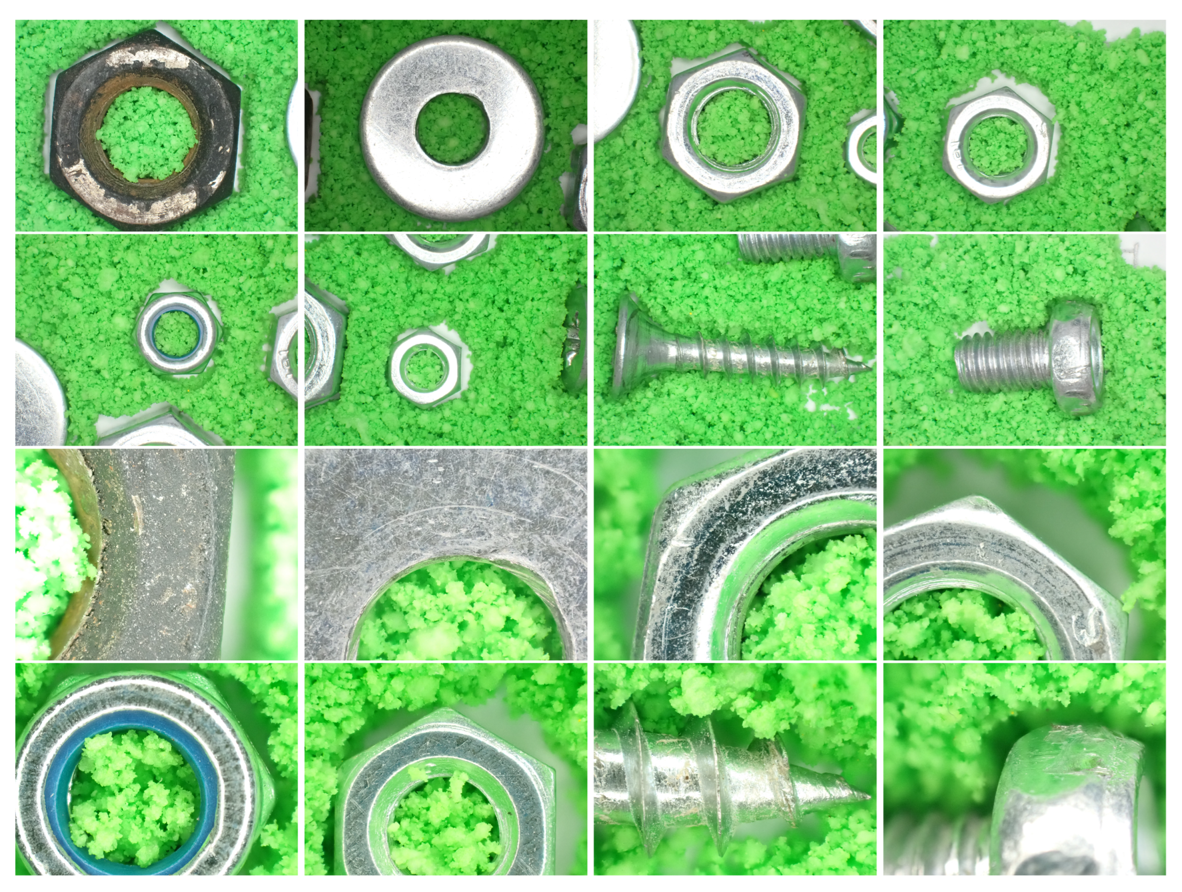
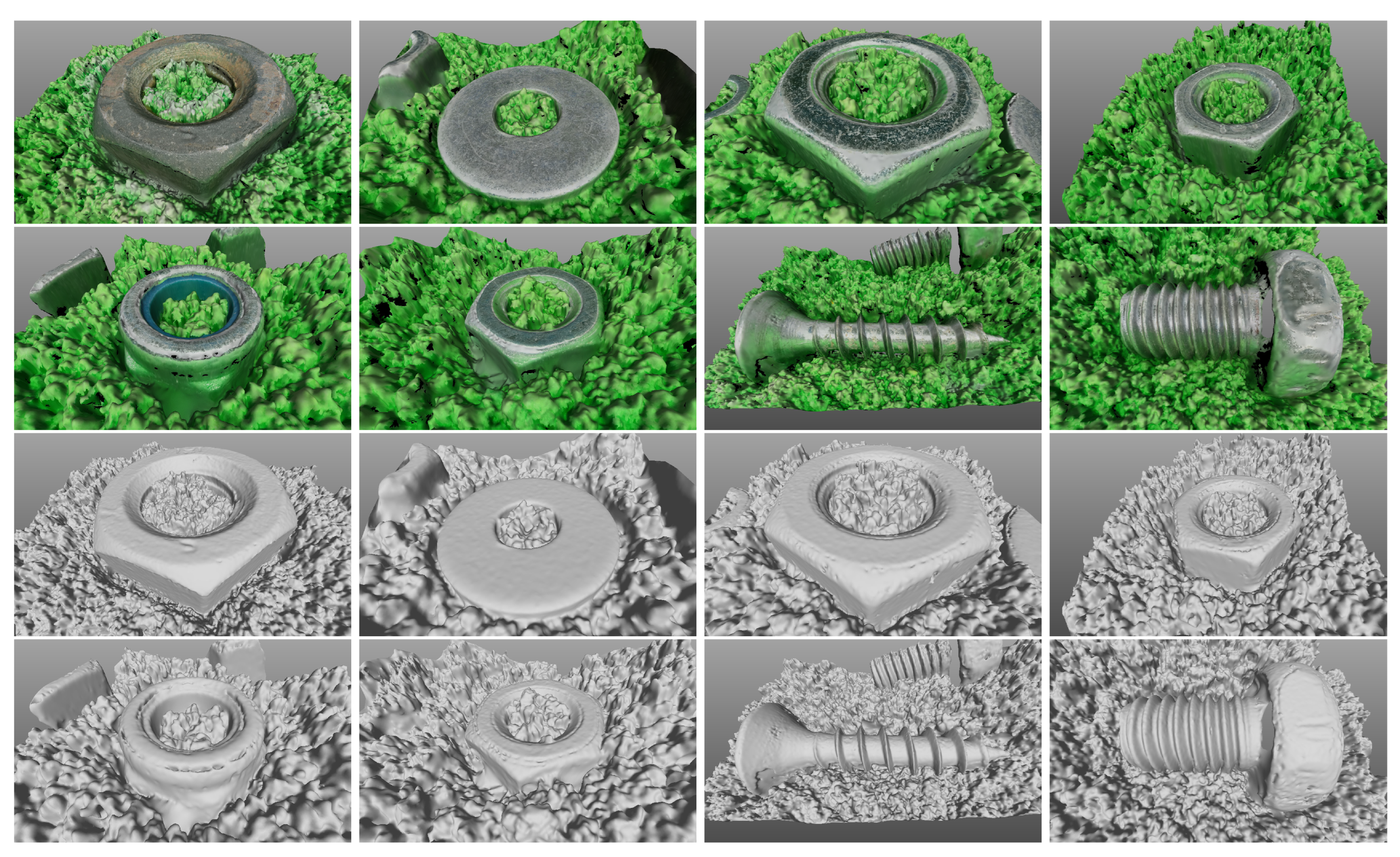
Figure 5.
Original images of metallic nuts and screws. The top couple of rows shows an original image of the target from the top layer. The bottom couple of rows shows an original image from the closest layer to the target
Figure 5.
Original images of metallic nuts and screws. The top couple of rows shows an original image of the target from the top layer. The bottom couple of rows shows an original image from the closest layer to the target
Figure 6.
Reconstructions of the metallic nuts and screws shown in Figure 5. The top couple of rows shows the textured reconstructions. The bottom couple of rows shows the untextured reconstructions from the same viewpoints.
Figure 6.
Reconstructions of the metallic nuts and screws shown in Figure 5. The top couple of rows shows the textured reconstructions. The bottom couple of rows shows the untextured reconstructions from the same viewpoints.
In Table 4, we compare the measured dimensions of the nuts and screws with their ground truth dimensions. The order of the measurement is the same as in Figure 5 and Figure 6. In this table, the first column reads the ground truth dimensions of the targets. The second column reads the dimensions of the target measured from the reconstruction. The third column reads the percentage error. For the six first rows, the dimensions reported are the diameter of the target, its thickness, and its height, in that order. The last two rows are different because they report screw measurements. In these rows, the first dimension reads the “height” of the screw (its longest dimension) and the second dimension reads the diameter of its “head”.
5. Conclusions and future work
A surface reconstruction approach and its implementation are proposed in the form of a surface scanning modality. The proposed approach employs image acquisition at multiple distances and feature tracking to increase reconstruction accuracy. The resultant device and approach offer a generic surface reconstruction modality that is robust to illumination specularities, is useful for several applications, and is cost-efficient.
This work can be improved to relax the limitation imposed by the restricted depth of focus range ( in our case) of the optical sensor. By revisiting the focused stacking method of Section 4.1, it is possible to acquire images at several distances and use the depth from focus visual cue [48] to coarsely approximate the elevation map of the surface. This approximation can be then used to scan the surface in a second pass, guiding the camera elevation appropriately so that the surface occurs within its depth of focus.
Finally, as active illumination supports photogrammetry, we aim to characterise the illumination types that are non-destructive for sensitive surfaces, per type of material. Although active illumination alters colour appearance, it is planned to acquire two images per viewpoint. The first, using structure light to facilitate photogrammetry. The second, from precisely the same viewpoint, would be to accurately capture the colour appearance.
Author Contributions
Conceptualization, X.Z., and P.K.; methodology, X.Z, P.K., and N.P.; software, P.K., and N.S.; validation, P.K., N.P., E.Z., and I.D.; data curation, P.K.; writing—original draft preparation, X.Z., P.K., N.S., N.P, E.Z., and I.D.; writing—review and editing, X.Z., P.K., N.S., N.P., E.Z., and I.D.; visualization, P.K., and X.Z.; supervision, X.Z., and N.P.; project administration, X.Z., and N.P.; funding acquisition, X.Z., and N.P. All authors have read and agreed to the published version of the manuscript.
Funding
This work was supported by the Horizon Europe Project, Craeft, Grant No. 101094349.
Institutional Review Board Statement
Not applicable
Data Availability Statement
The surface reconstructions shown in this work can be found at https://doi.org/10.5281/zenodo.8163498.
Conflicts of Interest
The authors declare no conflict of interest.
Abbreviations
The following abbreviations are used in this manuscript:
| AC-RANSAC | A Contrario RANSAC |
| b | byte |
| c | cent |
| CNC | Computer Numerical Control |
| CPU | Central Processing Unit |
| € | Euro |
| FoV | Field of View |
| G-code | Geometric Code |
| GHz | gigahertz |
| GPS | Global Positioning System |
| GPU | Graphics Processing Unit |
| HDD | Hard Disk Drive |
| ICP | Iterative closest point |
| JPEG | Joint Photographic Experts Group |
| OpenMVG | Open Multiple View Geometry |
| p | point(s) |
| ppi | points per inch |
| pix | pixel(s) |
| PNG | Portable Network Graphics |
| PLY | Polygon File Format |
| RANSAC | RANdom SAmple Consensus |
| RAM | Random-Access Memory |
| SIFT | Scale-Invariant Feature Transform |
| SD | Secure Digital |
| SSD | Solid-State Drive |
| USD | United States Dollar |
References
- Illerhaus, B.; Jasiuniene, E.; Goebbels, J.; Loethman, P. Investigation and image processing of cellular metals with highly resolving 3D microtomography (uCT). Developments in X-Ray Tomography III; Bonse, U., Ed. International Society for Optics and Photonics, SPIE, 2002, Vol. 4503, pp. 201 – 204. [CrossRef]
- Semendeferi, K.; Damasio, H.; Frank, R.; Van Hoesen, G. The evolution of the frontal lobes: a volumetric analysis based on three-dimensional reconstructions of magnetic resonance scans of human and ape brains. Journal of Human Evolution 1997, 32, 375–388. [Google Scholar] [CrossRef]
- Zabulis, X.; Koutlemanis, P.; Stivaktakis, N.; Partarakis, N. A Low-Cost Contactless Overhead Micrometer Surface Scanner. Applied Sciences 2021, 11. [Google Scholar] [CrossRef]
- Luhmann, T. Close range photogrammetry for industrial applications. ISPRS Journal of Photogrammetry and Remote Sensing 2010, 65, 558–569. [Google Scholar] [CrossRef]
- Rodríguez-Martín, M.; Rodríguez-Gonzalvez, P. Learning based on 3D photogrammetry models to evaluate the competences in visual testing of welds. IEEE Global Engineering Education Conference, 2018, pp. 1576–1581. [CrossRef]
- Rodríguez-Martín, M.; Rodríguez-Gonzálvez, P. Learning methodology based on weld virtual models in the mechanical engineering classroom. Computer Applications in Engineering Education 2019, 27, 1113–1125. [Google Scholar] [CrossRef]
- Fau, M.; Cornette, R.; Houssaye, A. Photogrammetry for 3D digitizing bones of mounted skeletons: Potential and limits. Comptes Rendus Palevol 2016, 15, 968–977. [Google Scholar] [CrossRef]
- Gajski, D.; Solter, A.; Gašparovic, M. Applications of Macro Photogrammetry in Archaeology. The International Archives of the Photogrammetry, Remote Sensing and Spatial Information Sciences 2016, XLI-B5, 263–266. [CrossRef]
- Marziali, S.; Dionisio, G. Photogrammetry and macro photography. The experience of the MUSINT II Project in the 3D digitizing process of small size archaeological artifacts. Studies in Digital Heritage 2017, 1, 298–309. [Google Scholar] [CrossRef]
- Hassett, B.; Lewis-Bale, T. Comparison of 3D landmark and 3D dense cloud approaches to hominin mandible morphometrics using structure-from-motion. Archaeometry 2017, 59, 191–203. [Google Scholar] [CrossRef]
- Inzerillo, L. Smart SfM: salinas archaeological museum. International Archives of Photogrammetry, Remote Sensing and Spatial Information Sciences 2017, 42, 369–374. [Google Scholar] [CrossRef]
- Fernández-Lozano, J.; Gutiérrez-Alonso, G.; Ruiz-Tejada, M.Á.; Criado-Valdés, M. 3D digital documentation and image enhancement integration into schematic rock art analysis and preservation: The Castrocontrigo Neolithic rock art (NW Spain). Journal of Cultural Heritage 2017, 26, 160–166. [Google Scholar] [CrossRef]
- Lussu, P.; Marini, E. Ultra close-range digital photogrammetry in skeletal anthropology: A systematic review. PloS one 2020, 15, e0230948. [Google Scholar] [CrossRef]
- Lavecchia, F.; Guerra, M.; Galantucci, L. The influence of software algorithms on photogrammetric micro-feature measurement’s uncertainty. International Journal of Advanced Manufacturing Technology 2017, 93, 3991–4005. [Google Scholar] [CrossRef]
- Gallo, A.; Muzzupappa, M.; Bruno, F. 3D reconstruction of small sized objects from a sequence of multi-focused images. Journal of Cultural Heritage 2014, 15, 173–182. [Google Scholar] [CrossRef]
- González, M.; Yravedra, J.; González-Aguilera, D.; Palomeque-González, J.; Domínguez-Rodrigo, M. Micro-photogrammetric characterization of cut marks on bones. Journal of Archaeological Science 2015, 62, 128–142. [Google Scholar] [CrossRef]
- Percoco, G.; Salmerón, A. Photogrammetric measurement of 3D freeform millimetre-sized objects with micro features: an experimental validation of the close-range camera calibration model for narrow angles of view. Measurement Science and Technology 2015, 26, 095203. [Google Scholar] [CrossRef]
- Shortis, M.; Bellman, C.; Robson, S.; Johnston, G.; Johnson, G. Stability of zoom and fixed lenses used with digital SLR cameras. ISPRS Symposium of Image Engineering and Vision Metrology, 2006, pp. 285–290.
- Galantucci, L.; Guerra, M.; Lavecchia, F. Photogrammetry Applied to Small and Micro Scaled Objects: A Review. International Conference on the Industry 4.0 Model for Advanced Manufacturing; Ni, J., Majstorovic, V., Djurdjanovic, D., Eds.; Springer International Publishing: Cham, 2018; pp. 57–77. [Google Scholar] [CrossRef]
- Galantucci, L.; Lavecchia, F.; Percoco, G. Multistack close range photogrammetry for low cost submillimeter metrology. Journal of Computing and Information Science in Engineering 2013, 13. [Google Scholar] [CrossRef]
- Mathys, A.; Brecko, J., Focus Stacking. In Digital Techniques for Documenting and Preserving Cultural Heritage; Amsterdam University Press, 2018; p. 213–216. [CrossRef]
- Galantucci, L.; Pesce, M.; Lavecchia, F. A stereo photogrammetry scanning methodology, for precise and accurate 3D digitization of small parts with sub-millimeter sized features. CIRP Annals 2015, 64, 507–510. [Google Scholar] [CrossRef]
- Percoco, G.; Guerra, M.; Jose Sanchez Salmeron, A.; Galantucci, L.M.; S. Experimental investigation on camera calibration for 3D photogrammetric scanning of micro-features for micrometric resolution. International Journal of Advanced Manufacturing Technology 2017, 91, 2935–2947. [Google Scholar] [CrossRef]
- Percoco, G.; Modica, F.; Fanelli, S. Image analysis for 3D micro-features: A new hybrid measurement method. Precision Engineering 2017, 48, 123–132. [Google Scholar] [CrossRef]
- Sims-Waterhouse, D.; Piano, S.; Leach, R. Verification of micro-scale photogrammetry for smooth three-dimensional object measurement. Measurement Science and Technology 2017, 28, 055010. [Google Scholar] [CrossRef]
- Sims-Waterhouse, D.; Bointon, P.; Piano, S.; Leach, R. Experimental comparison of photogrammetry for additive manufactured parts with and without laser speckle projection. Optical Measurement Systems for Industrial Inspection X. International Society for Optics and Photonics, SPIE, 2017, Vol. 10329, p. 103290W. [CrossRef]
- Lavecchia, F.; Guerra, M.; Galantucci, L. Performance verification of a photogrammetric scanning system for micro-parts using a three-dimensional artifact: adjustment and calibration. International Journal of Advanced Manufacturing Technology 2018, 96, 4267–4279. [Google Scholar] [CrossRef]
- Galantucci, L.; Pesce, M.; Lavecchia, F. A powerful scanning methodology for 3D measurements of small parts with complex surfaces and sub millimeter-sized features, based on close range photogrammetry. Precision Engineering 2016, 43, 211–219. [Google Scholar] [CrossRef]
- Besl, P.; McKay, N.D. A method for registration of 3-D shapes. IEEE Transactions on Pattern Analysis and Machine Intelligence 1992, 14, 239–256. [Google Scholar] [CrossRef]
- C., Y.; Medioni, G. Object modelling by registration of multiple range images. Image and Vision Computing 1992, 10, 145–155. [CrossRef]
- Lourakis, M.; Zabulis, X. Accurate Scale Factor Estimation in 3D Reconstruction. International Conference on Computer Analysis of Images and Patterns; Springer-Verlag: Berlin, Heidelberg, 2013. [Google Scholar] [CrossRef]
- Lowe, D. Distinctive Image Features from Scale-Invariant Keypoints. International Journal of Computer Vision 2004, 60, 91–110. [Google Scholar] [CrossRef]
- Cheng, J.; Leng, C.; Wu, J.; Cui, H.; Lu, H. Fast and Accurate Image Matching with Cascade Hashing for 3D Reconstruction. IEEE Conference on Computer Vision and Pattern Recognition, 2014, pp. 1–8. [CrossRef]
- Fua, P. A parallel stereo algorithm that produces dense depth maps and preserves image features. Machine vision and applications 1993, 6, 35–49. [Google Scholar] [CrossRef]
- Fischler, M.; Bolles, R. Random Sample Consensus: A Paradigm for Model Fitting with Applications to Image Analysis and Automated Cartography. Communications of the ACM 1981, 24, 381–395. [Google Scholar] [CrossRef]
- Csurka, G.; Zeller, C.; Zhang, Z.; Faugeras, O. Characterizing the Uncertainty of the Fundamental Matrix. Computer Vision and Image Understanding 1997, 68, 18–36. [Google Scholar] [CrossRef]
- Moulon, P.; Monasse, P.; Perrot, R.; Marlet, R. OpenMVG: Open multiple view geometry. International Workshop on Reproducible Research in Pattern Recognition. Springer, 2016, pp. 60–74. [CrossRef]
- Moulon, P.; Monasse, P.; Marlet, R. Adaptive Structure from Motion with a Contrario Model Estimation. Asian Conference in Computer Vision; Lee, K.; Matsushita, Y.; Rehg, J.; Hu, Z., Eds. Springer, 2013, pp. 257–270. [CrossRef]
- Lourakis, M.; Argyros, A. SBA: A Software Package for Generic Sparse Bundle Adjustment. ACM Transactions on Mathematical Software 2009, 36. [Google Scholar] [CrossRef]
- Barnes, C.; Shechtman, E.; Finkelstein, A.; Goldman, D.B. PatchMatch: A Randomized Correspondence Algorithm for Structural Image Editing. ACM Transactions on Graphics 2009, 28. [Google Scholar] [CrossRef]
- Jancosek, M.; Pajdla, T. Exploiting visibility information in surface reconstruction to preserve weakly supported surfaces. International scholarly research notices 2014, 2014. [Google Scholar] [CrossRef] [PubMed]
- Hiep, V.; Labatut, P.; Pons, J.; Keriven, R. High Accuracy and Visibility-Consistent Dense Multiview Stereo. IEEE Trans. Pattern Anal. Mach. Intell. 2011, 34, 889–901. [Google Scholar] [CrossRef]
- Waechter, M.; Moehrle, N.; Goesele, M. Let There Be Color! Large-Scale Texturing of 3D Reconstructions. European Conference on Computer Vision; Springer International Publishing: Cham, 2014; pp. 836–850. [Google Scholar] [CrossRef]
- Cernea, D. OpenMVS: Multi-View Stereo Reconstruction Library. https://cdcseacave.github.io/openMVS, 2008. [Online; accessed 6-June-2021].
- Catmull, E. A subdivision algorithm for computer display of curved surfaces; The University of Utah, 1974.
- Marr, D.; Poggio, T. Cooperative Computation of Stereo Disparity. Science 1976, 194, 283–287. [Google Scholar] [CrossRef]
- Canny, J. A computational approach to edge-detection. IEEE transactions on pattern analysis and machine intelligence 1986, 8, 679–698. [Google Scholar] [CrossRef] [PubMed]
- Grossmann, P. Depth from focus. Pattern Recognition Letters 1987, 5, 63–69. [Google Scholar] [CrossRef]
| 1 | This is because surface points imaged in the periphery of the image are farther away from the camera than surface points imaged at the image centre. |
| 2 | G-code, or RS-274, is a programming language for numerical control, standardised by ISO 6983. |
| 3 | Polygon File Format (PLY), or Stanford Triangle Format, is a format to store 3D data from scanners. |
Figure 1.
Original images (top) and reconstructions of a silver, hand-carved spoon for two experimental conditions (middle, bottom).
Figure 1.
Original images (top) and reconstructions of a silver, hand-carved spoon for two experimental conditions (middle, bottom).
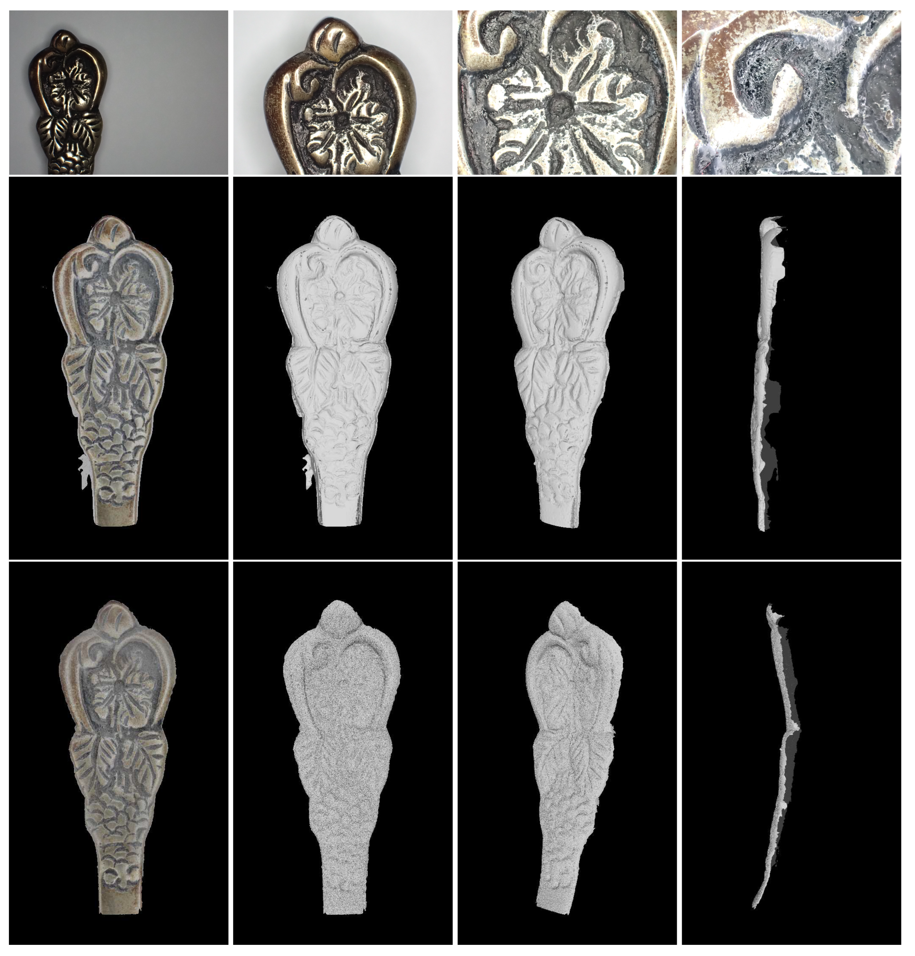
Figure 2.
Original images of circular coins. The top couple of rows shows an original image of the target from the top layer. The bottom couple of rows shows an original image from the closest layer to the target
Figure 2.
Original images of circular coins. The top couple of rows shows an original image of the target from the top layer. The bottom couple of rows shows an original image from the closest layer to the target
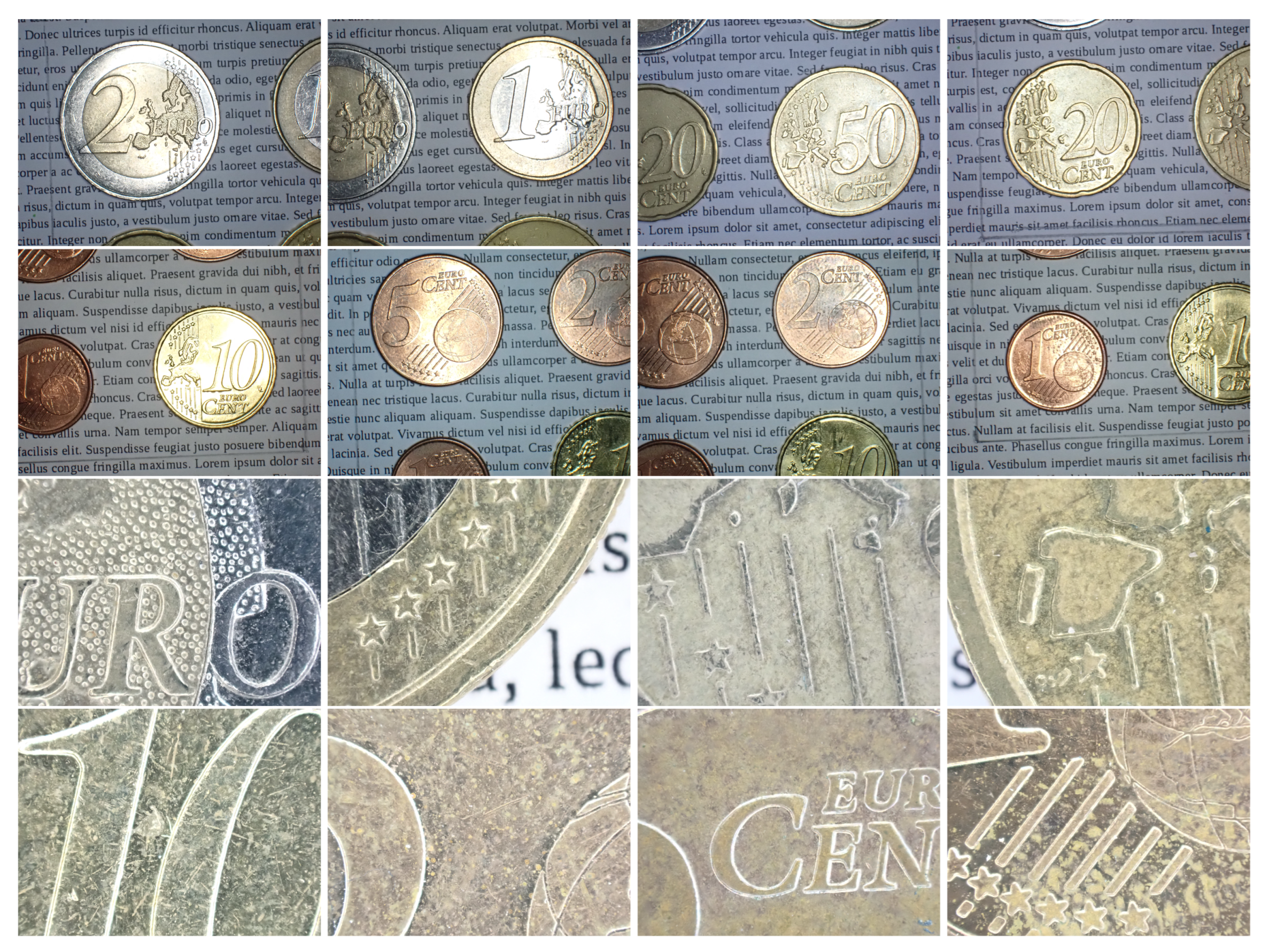
Figure 3.
Reconstructions of the circular coins shown in Figure 2. The top couple of rows shows the textured reconstructions. The bottom couple of rows shows the untextured reconstructions from the same viewpoints.
Figure 3.
Reconstructions of the circular coins shown in Figure 2. The top couple of rows shows the textured reconstructions. The bottom couple of rows shows the untextured reconstructions from the same viewpoints.
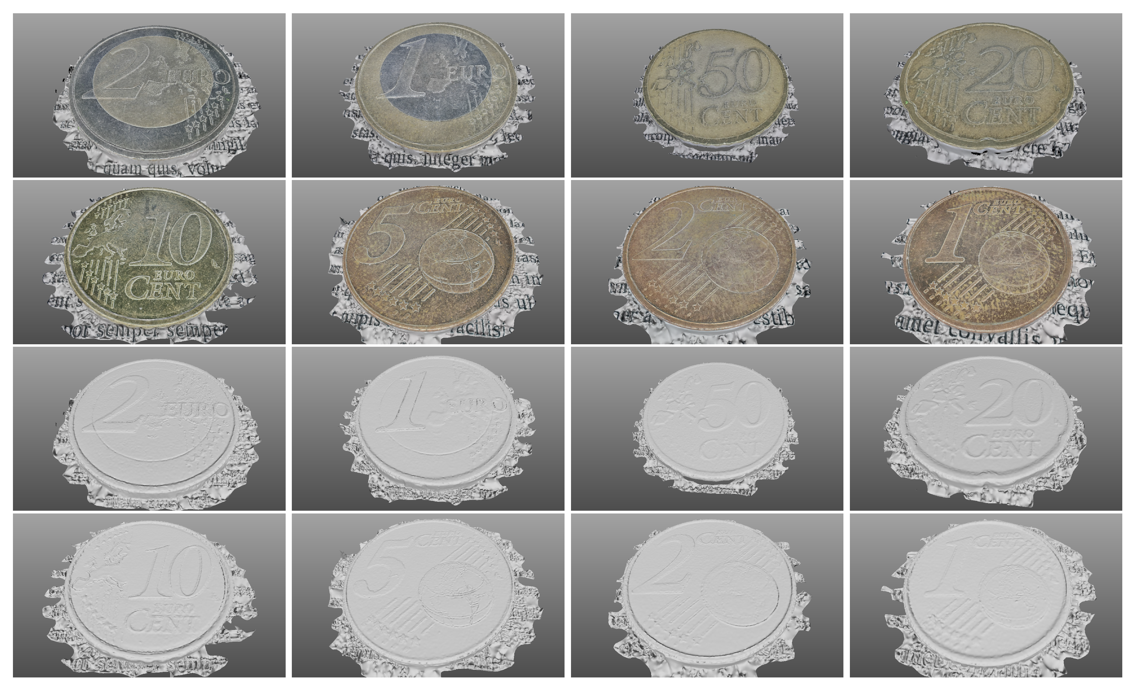
Figure 4.
Orthoimages of textured reconstructions superimposed with the depth edges employed in the assessment of reconstruction distortions.
Figure 4.
Orthoimages of textured reconstructions superimposed with the depth edges employed in the assessment of reconstruction distortions.
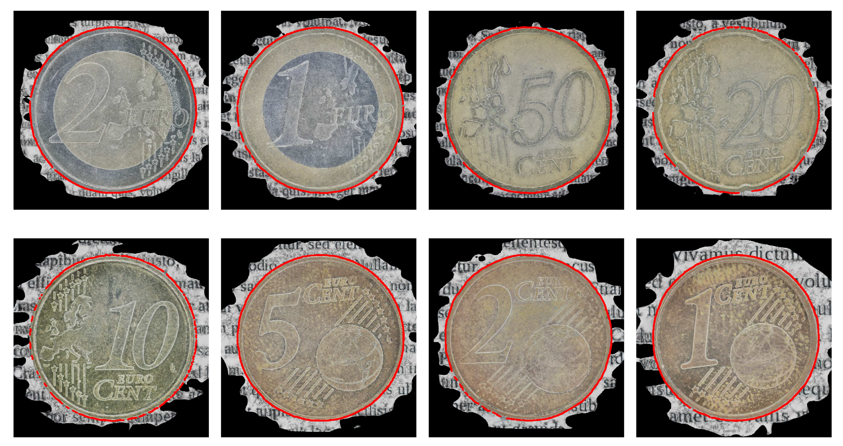

Table 1.
Spatial arrangement of camera locations in a square frustum structure.
| Layer | E () | n (#) | (#) | (#) | () | () | () |
|---|---|---|---|---|---|---|---|
| 1 | 160.0 | 50 | 5 | 10 | 4.51 | 3.38 | 11.296 |
| 2 | 80.0 | 551 | 19 | 29 | 2.25 | 1.69 | 5.648 |
| 3 | 40.0 | 3102 | 47 | 66 | 1.12 | 0.84 | 2.824 |
| 4 | 20.0 | 14420 | 103 | 140 | 0.56 | 0.42 | 1.412 |
Table 2.
Coin dimensions (diameter × thickness), measured dimensions, and percentage measurement errors ().
Table 2.
Coin dimensions (diameter × thickness), measured dimensions, and percentage measurement errors ().
| Currency | Dimensions () | Measurement () | Error (%) |
|---|---|---|---|
| 1c | |||
| 2c | |||
| 5c | |||
| 10c | |||
| 20c | |||
| 50c | |||
| €1 | |||
| €2 |
Table 3.
Radius, mean circle fit error, and standard deviation, in pixels, for each measured coin.
| Currency | Radius (p) | Error, std (p) |
|---|---|---|
| 1c | 224.58 | 0.49 (0.38) |
| 2c | 243.45 | 0.69 (0.41) |
| 5c | 232.66 | 0.48 (0.35) |
| 10c | 234.63 | 0.67 (0.41) |
| 20c | 238.50 | 0.66 (0.43) |
| 50c | 248.21 | 0.51 (0.37) |
| €1 | 231.52 | 0.71 (0.40) |
| €2 | 237.88 | 0.41 (0.33) |
Table 4.
Measurements of nut and screw diameter measurements, manufacturer dimensions, and percentage measurement errors ().
Table 4.
Measurements of nut and screw diameter measurements, manufacturer dimensions, and percentage measurement errors ().
| # | Dimensions () | Measurement () | Error (%) |
|---|---|---|---|
| 1 | |||
| 2 | |||
| 3 | |||
| 4 | |||
| 5 | |||
| 6 | |||
| 7 | |||
| 8 |
Disclaimer/Publisher’s Note: The statements, opinions and data contained in all publications are solely those of the individual author(s) and contributor(s) and not of MDPI and/or the editor(s). MDPI and/or the editor(s) disclaim responsibility for any injury to people or property resulting from any ideas, methods, instructions or products referred to in the content. |
© 2023 by the authors. Licensee MDPI, Basel, Switzerland. This article is an open access article distributed under the terms and conditions of the Creative Commons Attribution (CC BY) license (http://creativecommons.org/licenses/by/4.0/).
Copyright: This open access article is published under a Creative Commons CC BY 4.0 license, which permit the free download, distribution, and reuse, provided that the author and preprint are cited in any reuse.


