Submitted:
20 July 2023
Posted:
21 July 2023
You are already at the latest version
Abstract
A macro network loading Model for multi-flow lines, time-varying and pedestrian congestion is proposed. The station hub is abstracted as a network of different types of nodes, and the flow of passengers at each node is calculated in real time for the purpose of simulating the hub's collection and distribution process. For correct transmission of passenger flow on heterogeneous networks, three types of indexes are proposed to distinguish the nodes, and then match the corresponding fundamental diagrams. This paper divides the update process of the dynamic network loading model into multiple processes by flow lines, and improves computational speed of DNL model. The proposed model is applied to the simulation of passenger flow collection and distribution in an actual hub station with multi-flow lines. The analysis results illustrate that the model can accurately reflect the realistic congestion facilities and explain the formation process of high-density areas. A rolling passenger flow control model based on optimal control theory is proposed. The effectiveness of the control model is verified based on simulation data.
Keywords:
Macroscopic Pedestrian Flow Model
; Passenger Collection and Distribution
; Dynamic network loading model
; Optimal control theory
1. Introduction
There is a general need to better understand pedestrian traffic in densely populated areas such as airports, hub stations, shopping malls or other busy sidewalks. For important transportation infrastructures such as hub stations, the features of pedestrian flow collection and distribution are related to whether they can achieve their main functions. Thus, the pedestrian flow model is of great importance for traffic planning and design.
Pedestrian flow model is classified into micro model and macro model. The micro model takes individual pedestrians as the simulation object, and achieves the purpose of simulating crowd motion by calculating the velocity vector or transfer probability of multiple pedestrians at the same time. The method of continuity is represented by the social force model (Helbing1996), which describes the velocity vector of an individual pedestrian under the action of a wall or others through a system of differential equations. Discrete methods are often implemented based on grid(Muramatsu et al.1999) or cellular automata(Nagatani and Takashi.2009), which divide the pedestrian motion space into grids, and achieve the purpose of simulating pedestrian motion by discussing pedestrian following and preferences to quantify the transfer probability of pedestrians between girds. At present, the study of the micro passenger flow model is relatively mature, and the self-organizing phenomena(Johansson,Helbing,and Shukla 2007;Moussaïd et al.2009) such as stratification and zonation have been reproduced in complex situations such as counter flow. However, the computational cost of the micro model is geometrically related to the number of simulated pedestrians, so there are limitations for scenarios with large spatial scales or a large number of pedestrians. Thus, scholars are studying the macro model to serve the above limitations of the micro model. The macro model focuses on pedestrian flow, and the fundamental diagram of pedestrian flow is an important concept of the macro model. It reflects the relationship between the average velocity of pedestrians and the density of pedestrian flows. Early macro fundamental diagrams were based on measured studies, and early fundamental diagrams of pedestrian facilities in public areas were studied by Older(1968); Lam, Lee, and Cheung (2002)studied the fundamental diagram of pedestrian flow in the subway based on the data of pedestrian facilities in Hong Kong and fitted the analytical formula of the fundamental diagram; Burghardt, Seyfried, and Klingsch(2013)specifically studied the fundamental diagram of pedestrians going up and down stairs, and these measured studies provided the basis for macro pedestrian flow simulation model. The continuous medium model(Hughes2002)is a representative of macro simulation models, and he extracted the pedestrian motion law into three criteria of density-determined velocity, pedestrian destination movement trend, and minimum movement cost, which promoted the development of the continuous medium model through simple and reasonable assumptions. The continuous medium model is composed by a set of differential equations, Huang et al.(2009) reviewed Hughes' study and further proposed a fast solution method for partial differential equations. Specifically, Hoogendoorn and Bovy (2003)proposed a target generalized function based on the pedestrian flow velocity vector for heterogeneous pedestrian flows, which accurately reproduces the pedestrian self-organization phenomenon and is even often used as a benchmark model for microscopic methods. Simplified macro models are generally used to solve traffic simulation problems in large scale cases, The Cellular Transmission Model proposed by Daganzo (1994) and the Link Transmission Model proposed by Yperman, Logghe,and Immers (2005)are representatives of simplified macro models. They abstract the real transportation system as a network or grid model, thus establishing connections between transportation facilities; Based on the fundamental diagram of traffic flow, large-scale traffic volume simulation is achieved by calculating traffic volume changes on nodes or grids.
In recent years, simplified macro models have been applied to the study of pedestrian flow, e.g., Asano, Iryo, and Kuwahara(2010)used CTM to simulate typical complex pedestrian flow situations such as crossings, opposite directions, and corners, and he pointed out that attention should be paid to the effect of heterogeneous pedestrian flow on the fundamental diagram, but did not explicitly introduce the mechanism of its implementation; Guo, Huang, and Wong(2011)also conducted a similar study. In the above study, the simplified macro model was applied to the same cases as the micro model, which didn't reflect the advantage of the low computational cost of the macroscopic model. At present, scholars aim to integrate the advantages of micro and macro models and propose a hybrid model with both accuracy and scale advantages. For example, Abdelghany et al.(2016)proposed a dynamic network loading model and a cellular automata model for the top and bottom layers, respectively, for pedestrian flow simulation with different resolutions, and their simulation results matched the measured passage bottlenecks and high-density areas of the Mecca pilgrimage site. Zhang and Jia(2021) and Wang et al.(2023) proposed hybrid model combining CTM and CA to simulate the pedestrian flow evacuation scenarios for large places with multiple exits and fire situations, respectively. The top layer of these hybrid models typically uses a network or grid structure to model the site as a whole, which can then be simulated by using a simplified macro model. While the network structure has better generalizability than the grid, the traffic flow simulation model approach on the network structure is known as dynamic network loading model (DNL), From this, the DNL has some theoretical significance for the development of hybrid models.
At present, the pedestrian flow DNL applicable on the meso scale still needs to be studied, and the fundamental diagram adaptation of nodes and the choice preference of pedestrians in the case of heterogeneous pedestrian flow are currently the focus of scholars. Hänseler et al.(2017)proposed a DNL model for heterogeneous pedestrian flows based on the idea of CTM, which has a specially designed velocity-density fundamental diagram that can adaptively implement the consideration of pedestrian flow crossings and counter cases according to the angle between pedestrian flows, while they use Logit functions to calculate the selection preferences of pedestrians; Shang et al.(2021)considered pedestrian preferences with density and following effect, by using Decision Field Theory (DFT); Lilasathapornkit and Saberi (2022) defines a DUE problem for pedestrian path selection based on real-time passenger flow results from DNL and makes it applicable to heterogeneous pedestrian flow simulation. Different destinations of passengers are an obvious reason for heterogeneous pedestrian flow, which is fundamentally different from the path selection behavior of pedestrians, and there is a lack of dedicated discussion on this issue. The passenger collection and distribution in the hub station, is expressed as a flow line conflict, which can be summarized as pedestrians belong to different flow lines and are constrained by different transportation processes, and the path selection of passengers is based on the premise of satisfying the transportation process constraints. Current macro models are lacking to consider such heterogeneous traffic flow scenarios caused by multiple destinations of pedestrians. For example, Abdelghany's top network model has only one overall direction, which is suitable for a pass-through situation like the pilgrimage. Although Zhang and Wang discuss the evacuation scenario with multiple exits, the evacuation pedestrian flow can still be considered as homogeneous, and the reason for this is that the exits are homogeneous. Aghamohammadi and Laval (2020)reviewed pedestrian flow models in recent years, he pointing out the limitations of present models in heterogeneous traffic flow, multi-destination cases. Thus, there are still limitations in applying to traffic networks. Therefore, incorporating both the transport process constraints to be satisfied by pedestrians and the pedestrian selection preference factors into the propagation rules of the DNL model will help expand the application of the DNL model in the pedestrian flow collection and distribution cases.
Finally, the fundamental purpose of the pedestrian flow model is to provide a basis for traffic assignment, and then to achieve better traffic organization. In static traffic networks, this problem is known as the STA problem and has been well solved. By transforming the STA problem into a bi-level programming problem is the more general approach, loading different ODs randomly to the traffic network and the impedance function defined by the traffic volume is the crucial task. The user equilibrium principle is often used as the basis for determining the objective function of the optimization problem. The solution of the optimization problem is based on different types of heuristic approaches. Bielli et al. (2002)reviewed the application of genetic algorithms in bus route planning; Szeto and Jiang(2014)proposed an artificial bee algorithm for solving the STA problem of bus route planning; Kabir et al.(2023)solved a multi-objective road network evacuation problem by using a heuristic approach. This approach has major limitations when extended to Dynamic Traffic Assignment (DTA). In dynamic traffic networks, pedestrian flows cannot exist at all nodes on the link at the same time, so it is not sufficient to support the static assignment assumption; On the other hand, the random update method does not fundamentally solve the decoupling of update order and calculation results. and the DTA problem can be regarded as a variational problem. Based on the above analysis, we propose a systematic dynamic network loading model. It can be well applied to objects with such scale as hub stations and the presence of multi-directional pedestrian flow, so as to simulate the collection and distribution processes of passenger flow. The key problems addressed in this paper are as follows:
1. Based on the idea of CTM, a model is proposed for describing passenger collection and distribution in a single facility node, it is called the Passenger Propagation Model (PPM) in this paper, it uses pedestrian speed, density and capacity (flow rate), as parameters, enabling it to simplify calculations using fundamental diagrams, while adaptively matching different fundamental diagrams based on real-time passenger flow conditions.
2. Based on the PPM model parameters proposed above, a heterogeneous network model for describing hub stations is designed, and the PPM dynamic parameters such as the passenger number and density are designed in vector form to distinguish the passenger flow of different flow lines. Three indexes are designed to distinguish the types of facility nodes in the heterogeneous network and provide the basis for the fundamental diagram matching of the DNL model.
3.A DNL method is designed to achieve the purpose of running PPM synchronously on a large scale in a heterogeneous network of hub stations, and then to obtain the simulation of the overall passenger flow collection and distribution process in a large scale hub station. In this paper, we call this method the macro dynamics propagation model (MDPM), and the update process of MDPM is designed to be applicable to multiple processes to address the increased computational cost brought by considering node heterogeneity and the flow line constraints. The passenger arrival pattern of the Xipu hub station is obtained through an actual traffic survey and used as input to the MDPM, and the effectiveness of the MDPM is verified by comparing the simulation results with the actual situation.
4. Based on the simulation results of hub station collection and distribution, the existence of MFD is analyzed, and a system state-space equation that can describe the change of local network passenger flow in the short term is established, and then an adaptive optimal control model of passenger flow congestion is established to achieve the purpose of improving the hub network collection and distribution function.
2. Methods
The simulation method in this paper is summarized as follows: a realistic hub station is abstracted into a network model with facilities as nodes, and the passenger flow information of all nodes in the network is updated at the same time to finally achieve the purpose of simulating passenger collection and distribution.
The problem is divided into three sub-problems: 1) How to create a dynamic network for modeling a hub station 2) Rules for updating passenger flow information for an individual node 3) How to organize nodes in a heterogeneous dynamic network to update their own information simultaneously on a large scale.
We propose the Passenger Propagation Model (PPM) to describe the update rules of an individual node, and the parameters involved in this model are stored and updated in a dynamic network model; According to the requirements of PPM, we designed a network model capable of efficiently storing dynamic information generated by passenger collection and distribution and indexed static information capable of reflecting the heterogeneity of facility nodes; Finally, we propose the MDPM model for large-scale organization of nodes in heterogeneous networks to run PPM for the purpose of simulation of passenger flow collection and distribution at hub stations.
2.1. Passenger Flow Propagation Model (PPM)
The process of passenger collection and distribution at a hub station needs to be defined starting from the operation rules of the facility nodes. We propose the Passenger Propagation Model (PPM) for describing the interaction mechanism between nodes, and it is illustrated in Figure 1. Passenger flow is the medium of interaction between nodes. Based on the passenger flow, we can calculate the real-time passenger flow density or occupancy of a facility node, and then calculate the pedestrian speed and the passenger flow rate of the facility node through the fundamental diagram in real-time.
We collectively refer to the passenger flow density, passenger flow speed, and passenger flow rate of a node as capacity-related parameters, which are classified as node information. Traffic assignment related parameters refer to travelers' choice preferences, sink node status, and traffic guidance measures, which obviously describe the quantitative association between the node and its sink node, and they are classified as edge information.
Passenger selection preference refers to the passenger's tendency to travel towards nodes with higher average speed or lower energy consumption [9]; When the passenger flow at a node falls into severe congestion, its capacity will tend to zero and there will be no passengers willing to enter this node, we call this situation a sink node in an inflow failure state, and design a threshold value based on passenger flow density to judge the state of the sink node; In the internal traffic organization of the hub station, it is often used to prevent pedestrian flow congestion by restricting entry and accelerating passage, which are collectively called pedestrian flow guidance, and the rate of pedestrian flow guidance control is the key to passenger flow control.
The PPM can clearly explain the generation of congestion. According to the relationship of flow rate-density fundamental diagram, when the pedestrian density continues to grow, its flow rate does not grow in the same proportion, which then causes the stagnant return of passenger flow and aggravates the density growth; When the density critical value is reached, the growing passenger flow will instead cause the flow rate to decrease and finally lead to congestion. Also the model can explain the self-relieving process of congestion.
2.2. Network Model of the Hub Station
A hub station is abstracted as a network model by taking the facilities, equipment and sites involved in passenger distribution in the hub station as nodes and defining the edges by the spatial adjacency between nodes. Where N is the set of nodes, E is the set of edges, ND and ED are the data contained in the nodes and edges, and the specific design is illustrated in Table 1. The dynamic data need to be calculated and updated in each simulation cycle, it includes the parameters involved in PPM, such as passenger flow, average velocity and other traffic parameters belonging to a facility as node dynamic data, by considering the heterogeneity of node service mode, the parameters such as pedestrian flow density and occupancy rate are homogenized to the equal concept of node load. It satisfies the relationship that traffic capacity is equal to the product of load and operating efficiency.
The edge dynamic data describe the propagation weights of passenger flows between nodes, and we design three types of weight parameters with a value range of [0,1]:
w1 is the selection preference of passengers, who tend to prefer lower density nodes for higher proceeding speed, so w1 is the dynamic data updated based on the real-time passenger flow of the facility nodes.
w2 is the control rate corresponding to on-site traffic control or guidance measures, such as traffic restriction or guidance to speed up the flow of passengers.
w3 is the node failure weights, when the pedestrian flow density is above the critical value, the velocity decreases to 0 which can be considered as entering the failure state and assigned to 0. When it is below the critical value, the value is assigned to 1. Thus w3 is the dynamic data updated based on the real-time passenger flow of the facility node.
Static data exists only in nodes, including fixed attributes such as size and width of facilities nodes and three types of indexes for node classification. The size of the facilities and equipment is used to calculate the density with the real-time passenger flow, and the width is used to calculate the passenger flow variation with the node's capacity. type2 and type3 are used to distinguish the service conditions and upstream and downstream directions of nodes respectively, thus achieving the correct matching of the fundamental diagram.
Type1 is the node's transport process index, is the key to enable transportation process constraints. For example, the flow of the subway entry flow line can be summarized as follows: Arrival→security check→ticket check→ride, The transport processes involved in the facility nodes are sequentially numbered, so that the law of rising order can be used to represent the rule of transport processes, and the different flow lines with close spatial locations are interleaved and numbered, which are used to enhance their differentiation in the index of transport processes. For the flow line conflict case in Figure 2, the nodes that are shared by multiple flow lines are numbered with a sufficiently large number to ensure that they do not have an ascending relationship with any neighbor node.
In order to realize the simulation of passenger collection and distribution process of multiple flow lines simultaneously, we map the passenger flow as a dimensional vector with the number of flow lines, and the elements in the vector represent the passenger flow of the node corresponding to a certain flow line. Except for velocity, the other parameters used to calculate the passenger flow variation also have a vector form. Using the DGL framework's DGL graph class as the hub station network model G data structure, it can store tensor tuples and provide basic query functions to read and write any data in the network model simply by following the model →node/linked edge data→channel→node/linked edge index.
2.3. Macro Dynamics Pedestrian Flow Model (MDPM)
We describe the method of organizing nodes in a heterogeneous network to run the PPM simultaneously as the macro-dynamic pedestrian flow model(MDPM). Although PPM can provide a uniform description of the operation mode of each node, the heterogeneity of the nodes, the constraints of the transportation process, and the update method of the network are issues that must be considered.
2.3.1. Heterogeneity of the Nodes
Hub stations include not only pedestrian facilities that can be portrayed by fundamental diagrams, such as passageways, but also auto-pedestrian facilities and service facilities that can't be described by fundamental diagrams. For automated pedestrian facilities such as escalators and elevators, it is clear that occupancy is more reasonable to describe the impact of passenger flow on the facility, while the operating speed of automated pedestrian facilities is independent of pedestrian flow density. Similarly for gates, ticketing and other service facilities, the capacity is mainly affected by the average service time.
For pedestrian facilities, the fundamental diagrams that they satisfy should also be refined according to their direction of movement. According to Burghardt's study [8], the fundamental diagram of pedestrian flow up and down stairs is significantly different from that of horizontal facilities. Both of the above heterogeneous cases can be identified by type2 and type3.
2.3.2. Constraints on Transportation Process
We describe the case that several flow lines share a single facility node as a flow lines conflict. Obviously, pedestrian flow in multiple directions is bound to occur in the case of a flow line conflict, and Figure 2(a) illustrates a typical flow line conflict case. In this case, it is necessary to consider the situation of counter flow and cross flow caused by the inconsistent direction of pedestrian flow movement. On the other hand, the regularity of passenger flow in the exit flow is more obvious than that in the entrance flow. Even if two flow lines share a node for distribution, it is necessary to determine whether there is a flow lines conflict based on the real-time passenger flow.
Transportation process is an important attribute of flow lines, reflecting static traffic organization plan, which can't be ignored in a network of such scale as hub stations, and can't be approximated by diversion ratios. Figure 2(b) is a networked abstraction of Figure 2(a), where entering and exiting passenger flows merge in the conflict region and then are assigned to their respective sink nodes. Assigning the passenger flow from node 2 to node 6 would violate the transportation process constraint.
2.3.3. Key Issues MDPM needs to Address.
Finally, assuming that the pedestrian flow satisfies the FIFO rule, the passenger flow of a node at a certain moment is determined by its own outgoing and its neighboring incoming passenger flows, so the update order of the node has a large impact on the simulation results. We summarize the factors and solutions that need to be considered specifically for MDPM in Table 2.
(1) MDPM differentiates between static heterogeneity by reading type2 and type3.
(2) Based on the real-time node passenger flow data with type1, the propagation rules of the nodes are designed to achieve the purpose of considering the dynamic heterogeneity and transportation process constraints at the same time.
(3) Assuming that the passenger flow has a limited range of changes within a short period, the dynamic data is temporarily "frozen" as static data. The MDPM is divided into a calculation process and an update process, and the effect of the update order on the calculation results is eliminated by calculating the "frozen" static data.
2.3.4. Specific Method of MDPM
The calculation process of MDPM in one cycle is illustrated in Figure 3, which divides the simulation work into three stages: getting data, calculation process, update process, where getting data from the network model G to get the capacity data of each node at the last moment (Table 1), because the node for each flow capacity is a vector, so the capacity of all nodes is a matrix, which we call Pedestrian flow traffic assignments matrix B. In the calculation process, the update amount of passenger flow at the node at the current time is calculated based on B matrix, and since B is static data, the calculation order has no relationship with the calculation result. Use multi-process method to speed up the calculation process. After obtaining the real-time passenger flow changes, the calculation of traffic parameters such as density and velocity of the network model G in the order of Figure 1 is called the update process.
The example in Figure 2 is used to illustrate how MDPM satisfies the transportation process constraints. It can be seen from the figure that there are exit passenger flow and entrance passenger flow in the flow line conflict region, and the passenger flow vector has two non-zero elements., while the node belonging to only one flow line has one non-zero element at most. The transportation process constraint can be satisfied by ensuring that the incoming passenger flow at non-conflicting nodes that are not part of this flow line is zero. The get_sodes_info program is proposed to calculate the inflow passenger flow for a single flow line at a single node, and its pseudo-code is illustrated in Figure 4.
The principle of get_sodes_info is summarized as follows: combine the transportation process index type1 with the passenger flow vector to judge whether the passenger flow of the source node should be imported. There are only three cases between node i and its source node:
(1) Node i and its source are non-conflicting nodes, its propagation rule satisfies the law of ascending order of transportation process index, considering that there may be multiple paths of different lengths in a flow line, passenger flow is imported when the index difference between the transport process i and the source is less than 5.
(2) Node i is a conflicting node (type1=99), at this time, node i accepts incoming passenger flow from all source nodes in all directions.
(3) When the source node j of i is a conflicting node, the program will perform a recursive query on the source node of j. The set of source nodes of j with non-zero passenger flow is obtained. Use the mean value of the transportation process index in the set as the basis for judgment. The same approach is taken as in case 1.
Case 2,3 is illustrated by the example in conjunction with Figure 2. Node 4 in Figure 2(b) belongs to case 2 (line 12 in the pseudo-code), which accepts passenger flows from all source nodes in all directions; Node 5 corresponds to case 3 (line 14 in the pseudo code), and when propagating the exit flow line (blue flow line in Figure 2), it will check its source node (4) of the source node. And from Figure 2(c), it can be seen that the node with non-zero passenger flow at this time is 3. And the transport flow index (type1) of nodes 3 and 5 do not satisfy the propagation condition, so the blue passenger flow in node 4 is rejected to be transmitted to node 5. Thus, as long as the passenger flow is generated in the correct flow dimension, the passenger flow propagation process can be able to ensure that the transportation process constraints are satisfied. The inflow of passengers at the nodes is calculated by using formula 1.
As can be seen from Figure 3 and formula 1, the goal of the calculation process is to obtain the real-time passenger flow change matrix (number of flow lines × number of nodes) for each node in each flow line, and the calculation order does not affect the computational results. Therefore, this paper splits it into several independent sub-tasks by flow line and computes them by multiprocessing module in parallel.
The update process of MDPM is according to the calculation process of PPM, and parameters such as load (pedestrian flow density, occupancy), operational efficiency (average pedestrian speed, average service time), and capacity (flow rate) of nodes are updated. Determine whether the parameter being updated has the form of a vector with flow lines as dimensions according to Table 1.
The node heterogeneity described in Table 2 is considered through the actuating logic of fundamental diagram matching (LFM) in Figure 5.
type2 is used to identify pedestrian facilities from other service facilities.
type3 is used to identify horizontal and non-horizontal pedestrian facilities, matching the fundamental diagram proposed by Burghardt et al.(2013).
When the node facility is a horizontal facility, there may be multiple directions of pedestrian flow in the facility node, and the impact of flow line conflicts on the fundamental diagram should be considered. Based on a micro pedestrian flow model, Li et al.(2015) investigated the features of counter pedestrian flow, using the appearance of self-organization phenomena as a signal of the presence of interactions between pedestrians, and he found that self-organization phenomena occur steadily when the pedestrian density is above 0.64 ped/m2. Lam et al.(2002)and Navin(1969)both conducted an empirical study on the characteristics of the counter pedestrian flows in the unsymmetrical case, and they pointed out that when the ratio of counter pedestrian flows is less than (1:9), it will have a large impact on the pedestrian fundamental diagram, so this paper uses the above condition as the basis for judging the flow line conflict. The remaining cases are calculated using the fundamental diagram proposed by Lam et al.(2002). In summary, the speed-density fundamental diagram formulas are listed in Table 3.
The value domain and monotonicity of the fundamental diagram can cause simulation errors in MDPM. If the fundamental diagram of pedestrian flow is obtained by fitting the actual observed data, polynomial fitting or Gaussian fitting are the usual fitting methods. In the actual observation samples, the data for extreme cases may be lacking, and then the sample set needs to be enhanced by experiments or by literature surveys manually (e.g., pedestrian flow velocity tends to zero for pedestrian flow densities greater than 5 ped/m2). It is necessary to enhance the sample, which can expand the definition domain of the fundamental diagram and enhance the scope of application of the fundamental diagram. The monotonicity of the fundamental diagram function reflects the whole trend of pedestrian flow velocity and density. Figure 6 illustrates the function images of the fundamental diagram used in this paper in the interval [0,8]. All the curves except the black show a reasonable trend that the velocity decreases with higher density. The failure to perform sample enhancement and polynomial fitting methods are the main reason for this incorrect fundamental diagram. If the black curve is used as the fundamental diagram of MDPM, it will incur the serious error that the higher the density, the faster the speed, and this serious error will further trigger the error that the node passenger flow is negative. Thus it is transformed into a yellow curve with sample enhancement and a higher regression order.
On the other hand, traffic parameters such as velocity, density, and flow rate should satisfy the non-negative constraints, which are difficult to satisfy throughout the definition domain, even for the processed polynomial curves (yellow curves). When these parameters are negative, it results in a negative outflow from the node, resulting in a false passenger accumulation. Both first-order Gaussian fitting and “truncation” can be used to satisfy the non-negative constraint. From Figure 6, it can be seen that the monotonicity of the curves using the Gaussian fit (up and down staircase fundamental diagram) is significantly better than that of the curves using the polynomial fit. The “truncation” refers to assigning a positive value close to 0 (0.01 in this paper) to the velocity when the density is above a threshold (5.5 ped/m2 for horizontal pedestrian facilities and 2.7 ped/m2 for flow lines conflicts). The “truncation” is also applied to the update function for node passenger flow (update_c), in order to achieve the same purpose as taking the minimum result for the three calculations in CTM.
The capacity is calculated according to Formula 6, and the traffic assignment matrix B is composed of the capacity of the nodes in the network on each flow line.
Node inflow failure w3 is determined by threshold setting (greater than 6ped/m) based on the fundamental speed-density diagram.For nodes with flow line conflicts, we design it as 2.7ped/m. In this paper only the preference of passengers for open areas is considered, i.e., w1 is calculated through a logit function with density as the dependent variable. In particular, the sum of w1 between node 4 with flow lines conflict in Figure 2 (b) and its sink node is determined by the number of flow lines involved (2 in Figure 2), i.e., the flow lines are divided for Logit operations.
3. Simulation
We established a network model based on the real Xipu Hub to validate our simulation approach. Xipu Station is a comprehensive hub primarily served by the metro, connecting Chengdu Metro Line 2 and Line 6. As the starting station of Line 2, it is responsible for integrating various modes of transportation, including buses, pedestrian traffic, and high-speed rail. The Xipu Hub consists of a total of 9 flow lines, with facilities and equipment associated with each flow line as nodes. Directed edges are established in the direction of flow lines. The network model is illustrated in Figure 7(a).
Using video data, we investigated the random arrival patterns of passengers during off-peak and peak periods. The specific approach involved dividing the arrival intervals into multiple intervals and calculating the frequency of passenger arrivals falling into each interval based on the video data. Figure 7(b) illustrates this process. Assuming that passenger arrivals follow an Erlang distribution, a random number generator can be designed based on Figure 7(b) to simulate random passenger arrivals. For subway systems with a predefined schedule, passenger flows are generated based on fixed simulation periods determined by the train intervals.
3.1. The Collection and Distribution during Off-Peak Period at Xipu Hub
Similarly, the passenger flow of virtual nodes is eliminated in a fixed period or every period to simulate the departure behavior of passengers. These "virtual" nodes connect the arrival and departure areas within the hub station, and they have an infinite area, thus avoiding node failure. By analyzing the arrival and departure situations at the virtual nodes, the average travel time of passengers within the hub can be calculated. Due to the stochastic nature of passenger arrivals and departures, multiple sets of experiments were conducted based on the arrival and departure situations during peak and off-peak periods. In each simulation experiment, the passenger flows and passenger density at each node were recorded to reflect the overall collection and distribution process within the hub.
First, based on the arrival characteristics during the off-peak period, multiple simulation experiments were conducted, and the results are presented in Figure 8. From Figure 8(a), it can be observed that, except for a few nodes, the passenger flow at most nodes tends to stabilize after reaching an equilibrium value. This is indicated by a relatively small variation in passenger flow, showing a trend towards a straight line. The "sawtooth" pattern in the passenger flow curve is caused by the choice behavior of MPMD (multi-path multi-destination) passengers or the mechanism of node inflow failure, and the specific reasons need to be evaluated in conjunction with real-time passenger density. Some nodes in the graph show a monotonic increase in passenger flow, indicating passenger congestion at these nodes. A typical example is Node 147. According to the query, node No. 147 is a bus platform located on the side of the Xipu Hub.
The local network topology of Node 147 is illustrated in Figure 8(b). This area includes four flow lines: Metro Line 2 outbound passenger flow, non-motorized vehicle arrival-bus departure, pedestrian arrival-bus departure, and long-distance inbound passenger flow. These flow lines are connected through two conflict areas, labeled as Node 15 and Node 29. The outflow of the target node is constrained by the passage capacity of the conflict area node (Node 15). When Node 15 experiences inflow failure, passenger congestion occurs, leading to an increase in the passenger flow at the target node.
Therefore, flow line conflicts are the cause of passenger congestion. Figure 9 presents a density (a) and passenger flow (b) heatmap based on real-time values in this simulation experiment. It is evident that the real-time passenger density at Node 145 remains within a healthy range, indicating that its passage capacity is in normal condition.
As Node 145 only has an edge connection to Node 15, its flow distribution weight (w1) is always 1. According to formula (1), the flow inflow failure weight (w3) is the fundamental reason for the passenger congestion. From Figure 9(a), it can be observed that the destination node's hub node, Node 15, consistently maintains a high level of passenger density, indicating inflow failure. This makes it challenging for Node 147 to route its passenger flow to Node 15.
One feasible approach to alleviate the passenger congestion at Node 147 is to enhance the passage capacity of Node 15. Two strategies can be implemented: Firstly, increasing the exit width of Node 15 to allow for a greater outflow of passenger flow to its hub node under the same unit passage capacity; Secondly, enhancing the evacuation capacity of departure nodes. Figure 10 illustrates the results of this simulation, showing that both strategies effectively alleviate the passenger congestion at Node 147, based on the results obtained from multiple simulations.
Based on Figure 9(a), it can be observed that the local network centered around Node 82 has a relatively high average passenger density. After further investigation, it was found that Node 82 represents the security checkpoint facilities of Metro Line 6 (assuming operational efficiency is independent of passenger density). From Figure 8(a) and the situation shown in Figure 10, it is evident that the passenger flow at Node 82 exhibits a “sawtooth” pattern, stabilizing within the range of [60, 70]. Considering its passenger density, it has not entered the state of inflow failure. Therefore, the “sawtooth “characteristic is a result of passenger preference.
However, as Node 82 represents a service facility with a constant service capacity, it is necessary to further increase passenger arrivals to discuss whether it becomes a bottleneck in passenger flow distribution during peak periods.
3.2. Collection and Distribution Characteristics Passenger Flow during Peak Period at Xipu Hub
Using the red curve in Figure 7(b) as the parameter for random passenger arrivals and the arrival interval of the subway in the dispersal direction is reduced to simulate the collection and distribution process of Xipu Hub during peak period. The simulation results are shown in Figure 11(a). At the end of the simulation time, the overall passenger flow in the network during the peak period is significantly higher compared to the off-peak period (Figure 10), indicating that MDPM can accurately reflect the collection and distribution process of passengers under different arrival levels.
The passenger flow at nodes 29, 50, and 147 exhibits a strictly monotonic increasing trend, indicating that they have not reached their maximum capacity. In order to explore the limits of the hub's distribution capacity, we doubled the expected passenger arrivals. The simulation results are shown in Figure 11(b).
Obviously, under higher expected passenger arrivals, the passenger flow accumulates more rapidly and reaches a peak before stabilizing. In Figure 11(a) and (b), there is no significant difference in the peak passenger flow near nodes 29, 50, and 147. Additionally, the overall passenger flow in the network in Figure 11(b) is not double that of Figure 11(a). This indicates that the mentioned nodes are approaching their maximum capacity. The additional incoming passenger flow becomes congested within the virtual arrival-departure nodes. Therefore, the peak values observed in the simulation results can reflect the hub's maximum collection and distribution capacity.
Figure 11(c) and (d) correspond to the real-time passenger density of the two simulations, which is combined with the real-time passenger flow of nodes to analyze the bottleneck nodes that restrict the hub's collection and distribution capacity. Through comprehensive analysis, we have identified three typical patterns that contribute to the increase in the number of passengers at nodes. These patterns are summarized in Table 4, which provides the criteria for identification.
The first pattern is characterized by passenger congestion caused by inflow failure. A representative node for this pattern is Node 147. By comparing its peak passenger flow during the peak period with that during the off-peak period, it can be observed that during the peak period, the congestion of passengers caused by the capacity constraint of Node 15 becomes more prominent. However, in reality, the passenger density at Node 147 still falls within a healthy range, so there is no need for excessive concern.
The second type of bottleneck is caused by flow lines conflicts. Firstly, these nodes exhibit high passenger flow and density. Secondly, their congestion state shows a certain degree of propagation, resulting in an increase in passenger flow or density at neighboring nodes. Additionally, due to the consideration of node failure effects in this paper, the passenger flow and density curves of these nodes exhibit a “sawtooth” pattern. Representative nodes in this category include Node 15, Node 29, and Node 50. Flow lines conflict nodes can lead to the accumulation of passenger flow at other nodes, making them important targets for optimization.
The third type of bottleneck is caused by insufficient service capacity of facility nodes. The passenger flow curve at these nodes reaches its peak rapidly and remains at a certain level. If there are other nodes with the same flow attributes (Type 1), a distinct “sawtooth” pattern will appear, which is determined by the passenger selection mechanism of the MDPM. For example, node group 80-84 is the security check equipment for Line 6, node 101 is the entry gate for Line 6, and node 151 is the escalator for transferring to Line 2 in the downward direction. This phenomenon can be utilized to quickly identify service facilities that do not meet the demand.
4. Optimization
Based on the MPDM simulation results, it is evident that the accumulation of passenger flow or the increase in passenger density is caused by different factors. Therefore, optimization strategies need to be employed based on different mechanisms. Automated facilities such as security checks, ticket gates, automated ticketing machines, and escalators have their throughput determined by the average service time. According to the conclusion above, the criteria for optimization are stable passenger flow and relatively high passenger density. Improving the operational efficiency of these facilities can help achieve the optimization objectives.
4.1. Methods for Passenger Flow Control
The other two causes of passenger congestion identified in Table 4 present relatively complex scenarios. As the capacity of nodes follows the fundamental diagram law, their performance is determined by real-time passenger flows, making the optimization problem a typical Dynamic Traffic Assignment (DTA) problem. Variational Inequality(VI) and the Optimal Control Theory (OC) proposed by Pontryagin et al.(1960) are both feasible methods for DTA problems as variational inequality is the main feature of DTA problems. On the other hand, when considering DTA problems in a network context, it is reasonable to simplify homogeneous local networks as a whole, describing the overall traffic capacity of the region through macro fundamental diagrams(MFD). By implementing boundary control measures in congested areas, the objective of improving the overall system's traffic performance can be achieved. Daganzo and Geroliminis(2008) also pointed out that the homogeneity of nodes is a prerequisite for the existence of MFD. Therefore, before simplifying with the idea of MFD, the existence of MFD was discussed based on the simulation data results.
Based on the simulation results in Figure 11(d), we identify 14 nodes to be included in the scope of passenger flow control, with 15th node as the central point. These nodes are further categorized into congestion areas, control areas, and evacuation areas. The congestion areas are initially determined based on the nodes that have bidirectional connections with the 15th node, namely nodes 16 and 142. The control areas consist of nodes that are sinks for the congestion areas, while the relief areas consist of nodes that are sources for the congestion areas. The partitioning results are presented in Table 4.
According to Table 1, the real-time passenger flow values (C) and real-time capacity (F) of each region were analyzed to determine their underlying patterns. Here, represents the real-time passenger flow value of the control area, calculated using Formula 7. The real-time capacity of the regions was computed using Formula 8. Figure 12(a) depicts the relationship between the passenger flow and capacity of each region during a simulation experiment. It is observed that there is a clear correlation between the passenger flow and capacity in the control and relief areas. The passenger flow in the control area shows an increasing trend, while the capacity in the relief area exhibits a turning point as the passenger flow increases. Furthermore, the trends in the relief and control areas are more pronounced compared to the congestion area. This could be attributed to the size of the regions, as the relief area typically encompasses a larger number of nodes, leading to better convergence of the curves.
In the temporal domain, these changing trends are more easily explained. Figure 12(b) shows the differential of the ratio between the capacity and passenger flow for the three regions over time. From the figure, it can be observed that after 100 cycles, the system enters a stable state where the second derivative of the capacity for all three regions stabilizes. This finding is consistent with the analysis conclusions derived from Figure 12(a). The stability of the capacity derivatives indicates the feasibility of utilizing rolling predictions based on passenger flow. Assuming that F is a function of C, we can expand the function at a known point to approximate the function at any given time, as shown in Formula 9.
When the rate of change of F/C is small (as observed in Figure 12(b) after 100 cycles), the second-order term can be neglected, simplifying Formula 10. By using F/C as an approximation of the derivative of capacity with respect to passenger flow. Formula 10 allows us to predict the capacity at any given time using the known passenger flow and capacity at a reference time. The neglected second-order term determines the prediction accuracy. Figure 12(c) illustrates the results of predicting regional capacity using a first-order Taylor expansion, that is, at each moment, the traffic capacity calculated by MDPM is used as a reference point. It can be seen from the figure that Formula 10 can make a more accurate prediction when the second-order derivative of F to C is small.
Based on the above conclusions, a system equation can be established to describe the variation of passenger flow in the three regions over time. Assuming over a time interval T, the change in the number of passengers in a region is equal to the difference between the inflow and outflow of passengers. At any given time tx, the control area is:
Where:
u represents the passenger flow control rate from the control region to the congested region
t0 represents the reference point mentioned in Formula 12.
The sum of the capacities from the control region to the congested region. we can further specify Formula 11 as follows:
Similarly, we can define the rate of passenger flow change for the congested region and the evacuation region as shown in Formula 13 and 14:
The system equations (12, 13, 14) provide a deterministic form to describe the changes in passenger flow in the three regions. The form is determinate and the accuracy of the predictions depends on the selection of the reference point t0. From Figure 12 (b, c), it can be observed that when t0 is selected to be close to tx and is within a small interval after 100 periods, the system equations exhibit better predictive accuracy. Based on this observation, a rolling optimization control strategy is proposed. In this strategy, the start of each control period is chosen as the reference point t0, and it is assumed that the system behavior remains unchanged within a short control period. The reference point obtained from the MDPM model at that specific moment is then used to assign values to the system equations for optimization purposes.
The objective functional for congestion control in the congested region is proposed with the system equation constraints, as shown in Formula 15. Formula 15 defines a terminal-free form control task, which means that there is no need to specify explicit control objectives for the controller. Instead, by defining the terminal state, the controller autonomously searches for the control trajectory. In this paper, the terminal state implies reducing the passenger flow in the control and congested regions at the end of the control period, with a higher weight assigned to the urgency of relieving congestion in the congested region. Simultaneously, it aims to increase the passenger flow in the relief region to achieve an auxiliary purpose. In the integral term, we aim to minimize the controlled passengers and observe a decreasing trend in passenger flow in the congested region during the process of passenger flow control.
The weight of the integral term is determined by the control domain. When the control rate exceeds the range of [-1, 1], it is considered as an invalid control. Since the indirect numerical solution is used in this paper, it is difficult to discuss the extreme value of the Hamilton function within the control domain. Therefore, the weight of the objective functional is determined jointly by experimentation and the terminal term.
The initial values of the system equations are determined by the control start time t0, while the final values of the Co-state equation are obtained from the transversality condition. The iterative solution is performed using the algorithm shown in Figure 12(d). Figure 12(e), (f), and (g) illustrate the control rate, the number of algorithm iterations, and the control results within a specific control period, respectively.
It can be observed that the control rate remains within the control domain, and the algorithm converges rapidly with a strictly decreasing objective functional. The initial value of the iteration of the u is 0. The monotonicity of the target generalized function implies that the passenger flow control is effective. In terms of the control results, at the end of the control period, the passenger flow in the congested area decreases, and there is a tendency towards equilibrium between the control area and the congested area.
4.2. Optimization Results
The optimization results of the hub's collection and distribution process using two strategies, namely passenger flow control and improving service facility efficiency, are presented in Figure 13. Compared with Figure 11 (b) and Figure 13 (a), it can be seen that under the same arrival condition of passengers, the overall passenger flow in the hub after optimization shows a downward trend, and the control target node does not reach the peak value of equilibrium compared with that before optimization. This indicates that the hub can accept a larger influx of passenger flow.
Comparing Figure 11 (d) and Figure 13 (b), it can be observed that the optimization effect is more pronounced in terms of passenger flow density, and the operation efficiency of service facilities has improved the congestion of nodes 80 to 84. Meanwhile, the optimal control model has effectively improved the congestion near node 15 caused by flow line conflicts.
The average travel time of passengers within the hub was evaluated by comparing the cumulative arrivals and departures of passengers at the same time. The results are shown in Figure 13(c), where the cumulative difference before and after optimization shows an increasing and stable trend, respectively. This indicates that before optimization, the average travel time of passengers gradually increased due to passenger congestion, while after optimization, the travel time of passengers within the hub presents a stable trend.
5. Conclusion and Discussion
5.1. Conclusion
In this paper, a DNL model is proposed for networks with large scale and heterogeneity, which can realize the loading of passenger flow in heterogeneous transportation networks in real time and adaptively.
1) MDPM automatically matches reasonable fundamental diagrams for nodes by classifying index and real-time passenger flow.
2). Through recursive query, MDPM can autonomously judge passenger flow propagation rules by combining the process index rule and passenger flow vector, so as to realize the transportation process constraints.
3) Based on real-time passenger flow, the selection preferences of passengers and node failure factors are considered through real-time updates.
The effectiveness of MDPM is verified by the actual traffic survey results. The high-density areas and passenger aggregation areas in the simulation results are highly consistent with the actual data in the assembly and dispersion process of XI-PU hub stations. Meanwhile, MDPM can clearly explain the formation process of these phenomena. The results show that inbound flow conflicts and insufficient capacity of service facilities are the main reasons for the formation of access bottlenecks, so the traffic design and flow organization work is the focus of work to improve the overall service capacity of hub stations.
Three empirical conclusions from the implementation of MDPM:
1) Both MDPM and CTM use the fundamental diagram to calculate the real-time capacity of the nodes. The non-negative constraint on the parameters is an issue that should be given attention. When the passenger flow is low, the capacity may be higher than the actual passenger flow, followed by the error that the outflow is negative, which eventually leads to the abnormal accumulation of passenger flow. In CTM, the traffic volume is guaranteed to satisfy the non-negative constraint by , and the comparison mechanism is also designed to achieve the non-negative constraint in this paper.
2) Accounting for node heterogeneity and transportation process constraints introduces extensive real-time judgment mechanisms, which can significantly increase the computational cost of MDPM. In this paper, MDPM is divided into 9 independent processes by the flow lines for parallel computation. MDPM was tested under three platforms, Ryzen5900HS, i5-12500H, and i7-7800H, and the computational speed of MDPM in each CPU test has 7~8 times improvement, with i5-12500H having the fastest computational speed, from 103.53s/iter before parallelism to 12.353s/iter. From the results, the improvement in computational efficiency depends on the number of CPU physical cores.
3) The value and definition domains of the velocity-density fundamental diagram need special attention. The fundamental diagram is often derived by fitting the actual data, and the fitting results will have certain limitations when extreme cases of observations are not available. The fit must not only fit the actual data in the observed sample, but also reflect the trend of the average pedestrian speed with density in the overall monotonicity. The monotonicity of Gaussian fitting is better than that of polynomial fitting, so it should be used as the preferred fitting method. Sample enhancement should also be used to improve the applicability of the fundamental diagram.
In addition, we investigated the existence of MFD based on the simulation results, and the results showed that the relationship between passenger flow and capacity of the local network showed a stable trend after a certain number of passenger flows and simulation periods. Based on this, a system state equation for short-time prediction of passenger flow is established, and the accuracy of this system equation is significantly and positively correlated with the size (number of nodes) of the local network.
Based on the proposed system equations, an optimal control model to decongest the passenger flow in the congested area is established. The model uses a rolling optimization model, performs local linear approximation to the unknown MFD curve through first-order Taylor expansion, transforms the system equation into a set of undetermined coefficients, and then determines the coefficients through MDPM real-time passenger flow data. This control model greatly reduces the difficulty of modeling the system equations while ensuring prediction accuracy.
Through two strategies of passenger flow control and service efficiency improvement, the collection and distribution process of hub stations in peak periods is optimized. The results show that this hybrid strategy can significantly reduce the overall passenger flow density in the network, while the travel time of passengers in transit also shows a decreasing trend.
5.2. Limitations discussion
In this paper, the passenger flow density is taken as the only factor affecting the passenger path selection. In reality, the walking energy consumption factor is a non-negligible influence, and the logit function will be improved in the future research work to realize the consideration of the energy consumption factor. Also, we will improve the LFM by adding more classification indexes and calculating branches to make the basic graph matching more detailed.
The optimal control model proposed in this paper is solved by an indirect numerical method, which substantially improves the convergence speed of the algorithm compared with the direct method. However, this method still has limitations compared to the analytical method. In this paper, the weight coefficient of the target functional is obtained through experiments, and ensuring that the control rate falls into the interval [-1,1] in the majority of cases is an important basis for the determination of the weight coefficients. Because there is no analytical solution, it is difficult to discuss the monotonicity of the Hamiltonian function, and subsequently, bang-bang control cannot be achieved. In future research, the analytical solution form of the passenger flow control model will be derived from the system equation modeling and the solution path of the partial differential equations.
References
- Helbing, Dirk. “A Stochastic Behavioral Model and a ?Microscopic? Foundation of Evolutionary Game Theory.”. Theory and Decision 1996, 40, 149–79. [CrossRef]
- Muramatsu, Masakuni, Tunemasa Irie, and Takashi Nagatani. “Jamming Transition in Pedestrian Counter Flow.”. Physica A: Statistical Mechanics and its Applications 1999, 267, 487–98. [CrossRef]
- Nagatani, Takashi. “Freezing Transition in Bi-Directional CA Model for Facing Pedestrian Traffic.”. Physics Letters A 2009, 373, 2917–21. [CrossRef]
- JOHANSSON, ANDERS, DIRK HELBING, and PRADYUMN K. SHUKLA. “Specification of the Social Force Pedestrian Model by Evolutionary Adjustment to Video Tracking Data.”. Advances in Complex Systems 2007, 10, 271–88. [CrossRef]
- Moussaïd, Mehdi, Dirk Helbing, Simon Garnier, Anders Johansson, Maud Combe, and Guy Theraulaz. “Experimental Study of the Behavioural Mechanisms Underlying Self-Organization in Human Crowds.”. Proceedings of the Royal Society B: Biological Sciences 2009, 276, 2755–62. [CrossRef]
- S.J, Older. “Movement of Pedestrians on Footways in Shopping Streets.”. Traffic engineering & control 1968, 10, 160–163.
- Lam, William H., Jodie Y. Lee, and C. Y. Cheung. “A Study of the Bi-Directional Pedestrian Flow Characteristics at Hong Kong Signalized Crosswalk Facilities.”. Transportation 2002, 29, 169–92. [CrossRef]
- Burghardt, Sebastian, Armin Seyfried, and Wolfram Klingsch. “Performance of Stairs – Fundamental Diagram and Topographical Measurements.”. Transportation Research Part C: Emerging Technologies 2013, 37, 268–78. [CrossRef]
- Hughes, Roger L. “The Flow of Human Crowds.”. Annual Review of Fluid Mechanics 2003, 35, 169–82. [CrossRef]
- Huang, Ling, S.C. Wong, Mengping Zhang, Chi-Wang Shu, and William H.K. Lam. “Revisiting Hughes’ Dynamic Continuum Model for Pedestrian Flow and the Development of an Efficient Solution Algorithm.”. Transportation Research Part B: Methodological 2009, 43, 127–41. [CrossRef]
- Hoogendoorn, Serge, and Piet H.L. Bovy. “Simulation of Pedestrian Flows by Optimal Control and Differential Games.”. Optimal Control Applications and Methods 2003, 24, 153–72. [CrossRef]
- Daganzo, Carlos F. “The Cell Transmission Model: A Dynamic Representation of Highway Traffic Consistent with the Hydrodynamic Theory.”. Transportation Research Part B: Methodological 1994, 28, 269–87. [CrossRef]
- Yperman, I. S., S. Logghe, and L. H. Immers. 2005. “The Link Transmission Model: An Efficient Implementation of the Kinematic Wave Theory in Traffic Networks.” 10th EURO Working Group on Transportation Meeting, Poznan, Poland, 122–127.
- Asano, Miho, Takamasa Iryo, and Masao Kuwahara. “Microscopic Pedestrian Simulation Model Combined with a Tactical Model for Route Choice Behaviour.”. Transportation Research Part C: Emerging Technologies 2010, 18, 842–55. [CrossRef]
- Guo, Ren-Yong, Hai-Jun Huang, and S.C. Wong. “Collection, Spillback, and Dissipation in Pedestrian Evacuation: A Network-Based Method.”. Transportation Research Part B: Methodological 2011, 45, 490–506. [CrossRef]
- Abdelghany, Ahmed, Khaled Abdelghany, and Hani Mahmassani. “A Hybrid Simulation-Assignment Modeling Framework for Crowd Dynamics in Large-Scale Pedestrian Facilities.”. Transportation Research Part A: Policy and Practice 2016, 86, 159–76. [CrossRef]
- Zhang, Zhe, and Limin Jia. “Optimal Guidance Strategy for Crowd Evacuation with Multiple Exits: A Hybrid Multiscale Modeling Approach.”. Applied Mathematical Modelling 2021, 90, 488–504. [CrossRef]
- Wang, Ke, Weifeng Yuan, Weiqi Liang, and Yao Yao. “An Optimal Guidance Strategy for Fire Evacuations: A Hybrid Modeling Approach.”. Journal of Building Engineering 2023, 73, 106796. [CrossRef]
- Hänseler, Flurin S., William H.K. Lam, Michel Bierlaire, Gael Lederrey, and Marija Nikolić. “A Dynamic Network Loading Model for Anisotropic and Congested Pedestrian Flows.”. Transportation Research Part B: Methodological 2017, 95, 149–68. [CrossRef]
- Shang, Huayan, Siyu Sun, Haijun Huang, and Wenxiang Wu. “An Extended Dynamic Model for Pedestrian Traffic Considering Individual Preference.”. Simulation Modelling Practice and Theory 2021, 106, 102204. [CrossRef]
- Lilasathapornkit, Tanapon, and Meead Saberi. “Dynamic Pedestrian Traffic Assignment with Link Transmission Model for Bidirectional Sidewalk Networks.”. Transportation Research Part C: Emerging Technologies 2022, 145, 103930. [CrossRef]
- Aghamohammadi, Rafegh, and Jorge A. Laval. “Dynamic Traffic Assignment Using the Macroscopic Fundamental Diagram: A Review of Vehicular and Pedestrian Flow Models.”. Transportation Research Part B: Methodological 2020, 137, 99–118. [CrossRef]
- Bielli, Maurizio, Massimiliano Caramia, and Pasquale Carotenuto. “Genetic Algorithms in Bus Network Optimization.”. Transportation Research Part C: Emerging Technologies 2002, 10, 19–34. [CrossRef]
- Szeto, W.Y., and Y. Jiang. “Transit Route and Frequency Design: Bi-Level Modeling and Hybrid Artificial Bee Colony Algorithm Approach.”. Transportation Research Part B: Methodological 2014, 67, 235–63. [CrossRef]
- Kabir, Mohimenul, Jaiaid Mobin, Muhammad Ali Nayeem, Muhammad Ahsanul Habib, and M. Sohel Rahman. “Multi-Objective Optimization and Heuristic Based Solutions for Evacuation Modeling.”. Transportation Research Interdisciplinary Perspectives 2023, 18, 100798.
- Daganzo, Carlos F., and Nikolas Geroliminis. “An Analytical Approximation for the Macroscopic Fundamental Diagram of Urban Traffic.”. Transportation Research Part B: Methodological 2008, 42, 771–81. [CrossRef]
- Pontryagin, L.S. Mathematical theory of optimal processes, 2018. [CrossRef]
- Li Ming-Hua, Yuan Zhen-Zhou, Xu Yan, and Tian Jun-Fang. “Randomness Analysis of Lane Formation in Pedestrian Counter Flow Based on Improved Lattice Gas Model.”. Acta Physica Sinica 2015, 64, 018903. [CrossRef]
- Navin, Francis P., and Robert J. Wheeler. "Pedestrian flow characteristics.". Traffic Engineering, Inst Traffic Engr 1969, 39. https://trid.trb.org/view/116327.
Figure 1.
Illustration of PPM model.
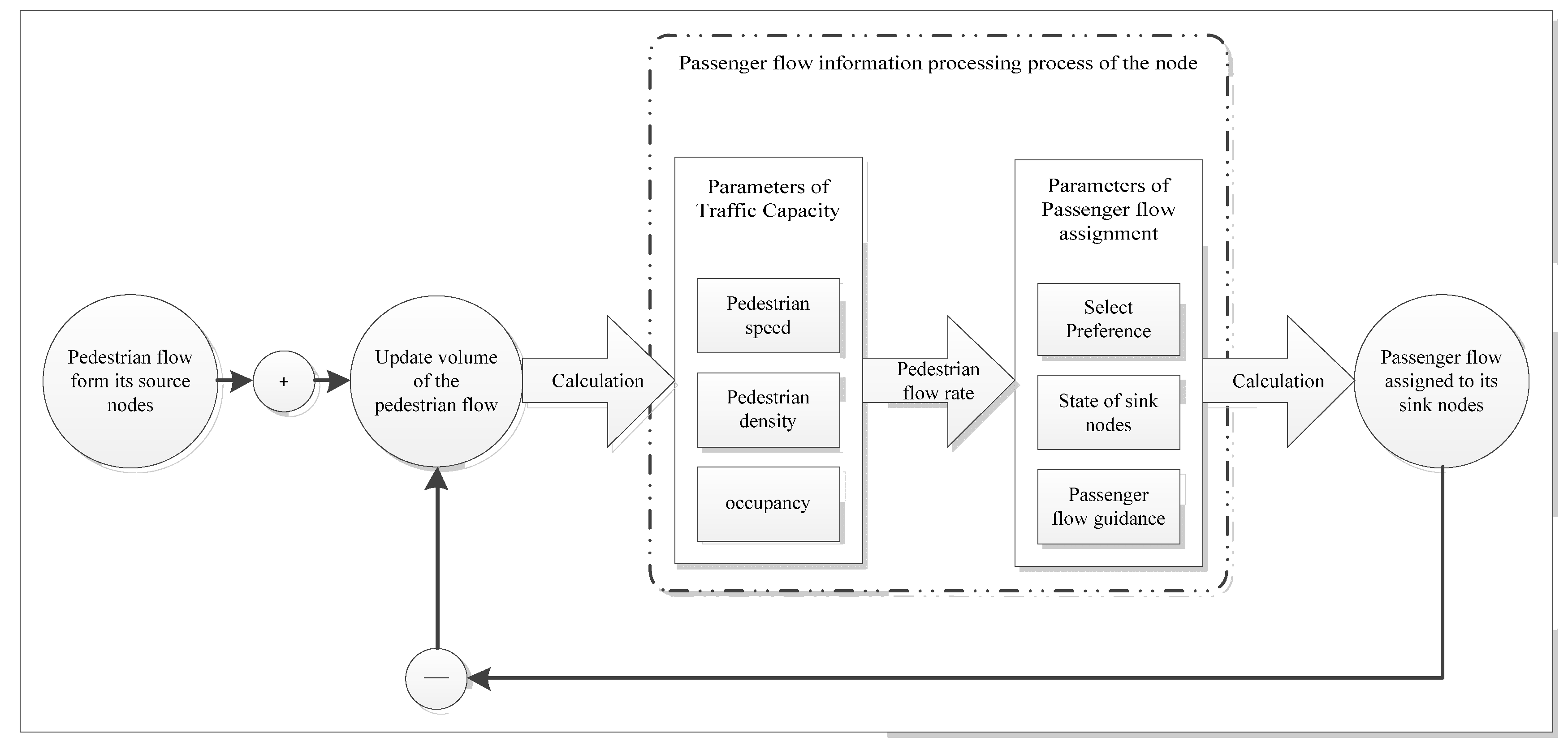
Figure 2.
Flow lines conflict.
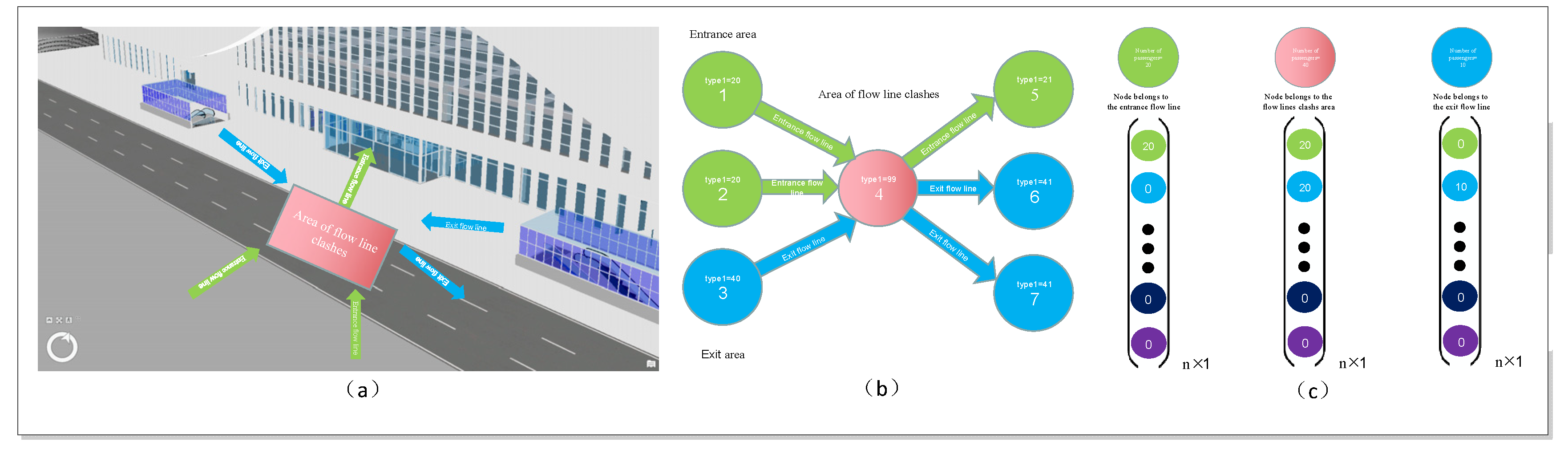
Figure 3.
MDPM calculation process.
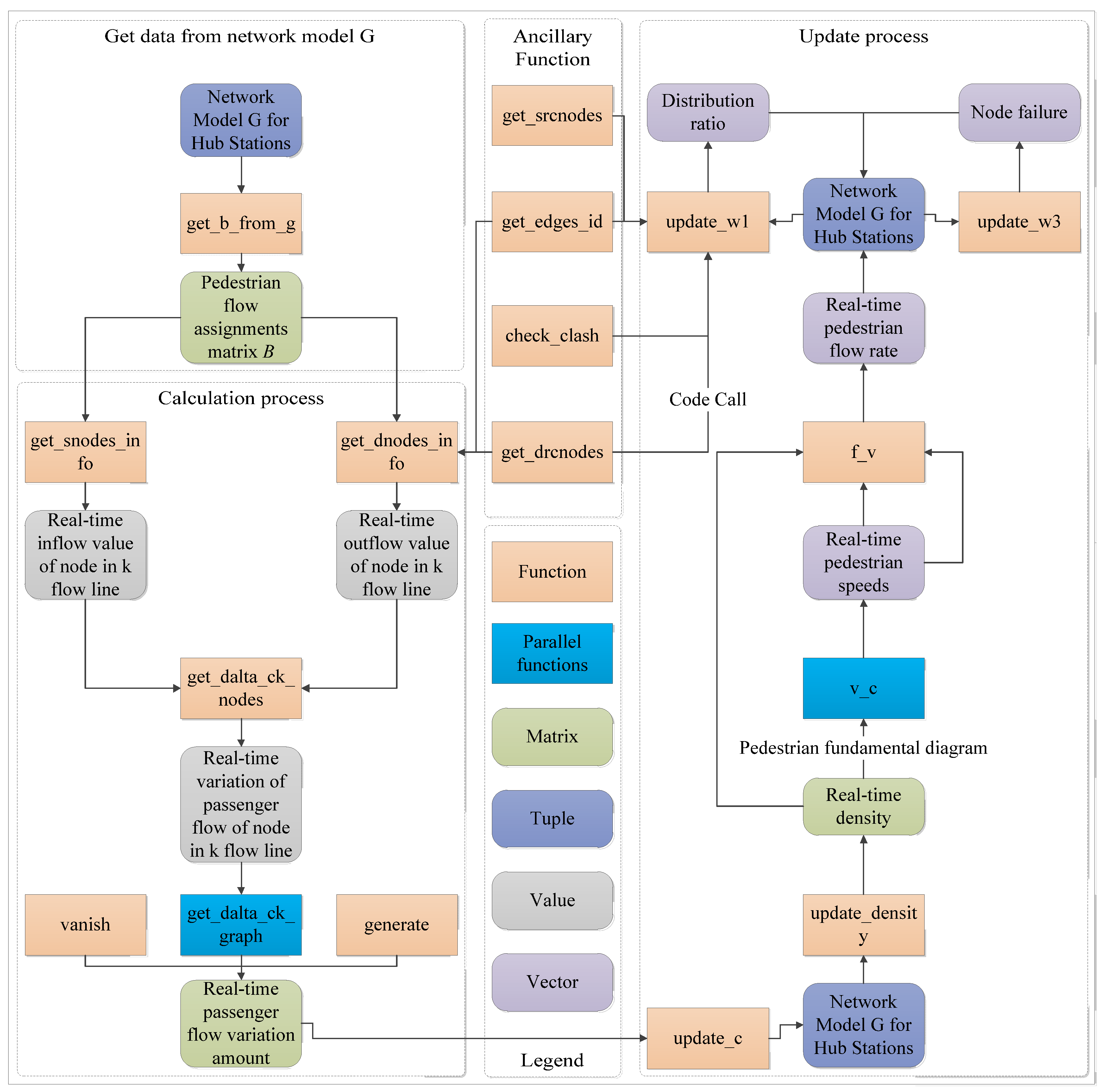
Figure 4.
Update pseudo-code for passenger inflow satisfying transportation process constraints.
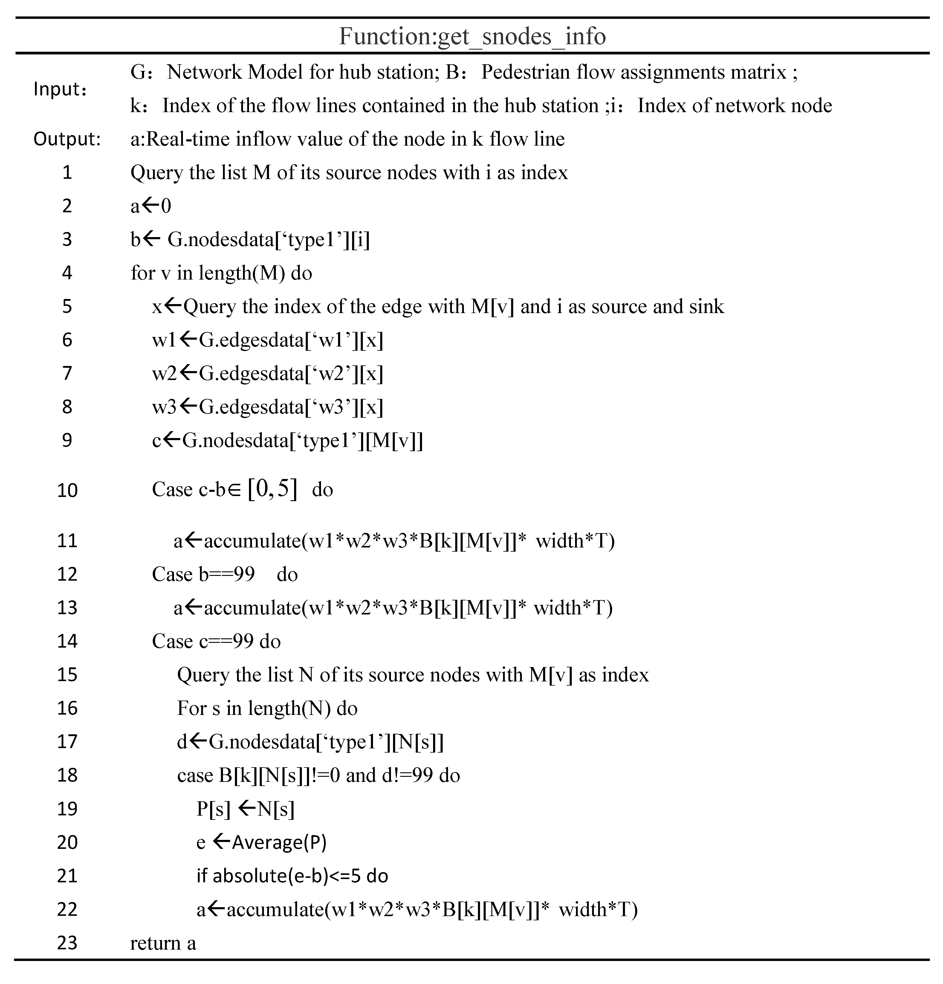
Figure 5.
The actuating logic of fundamental diagram matching(LFM).
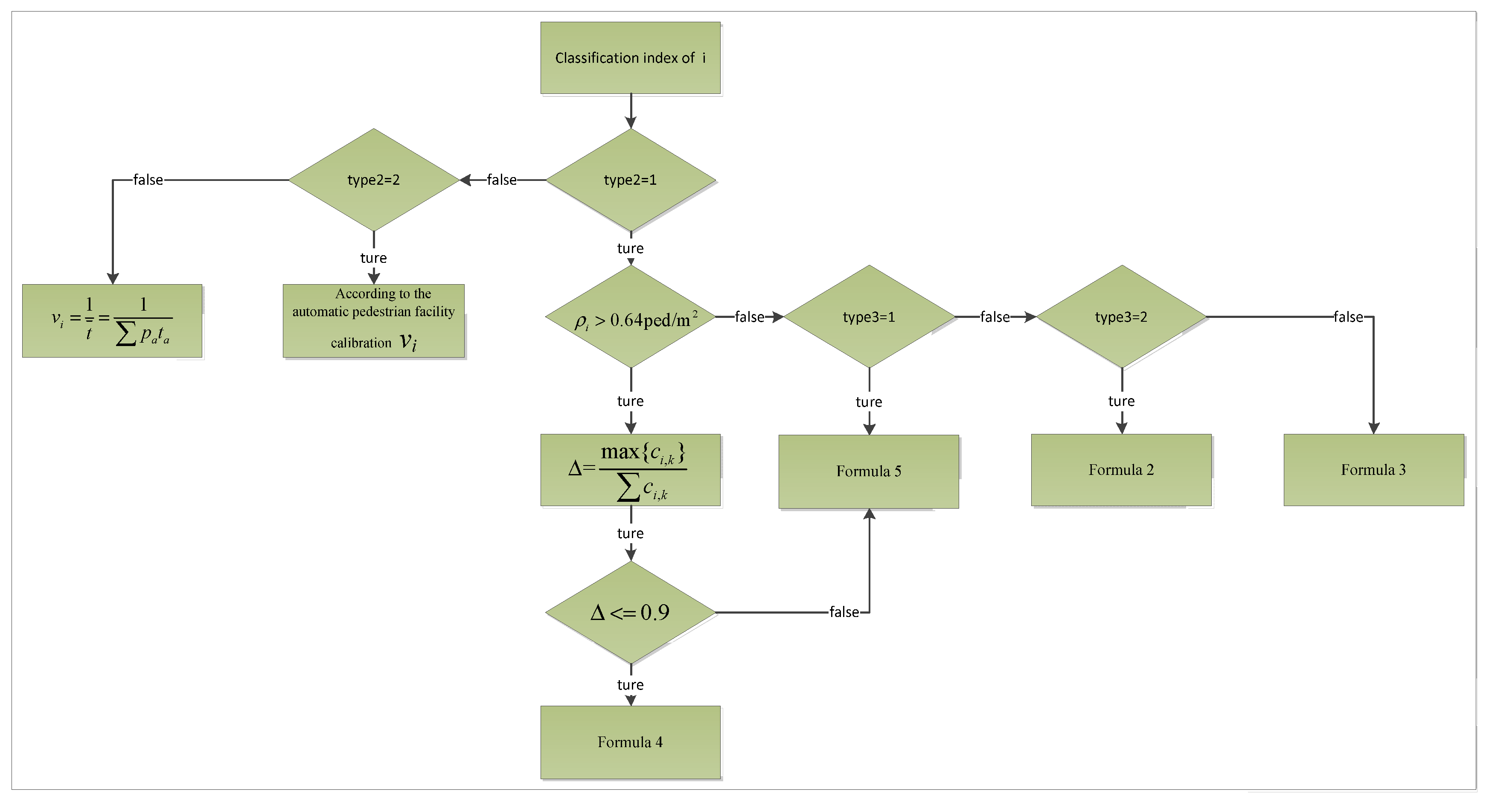
Figure 6.
The fundamental diagram curves used by MDPM.
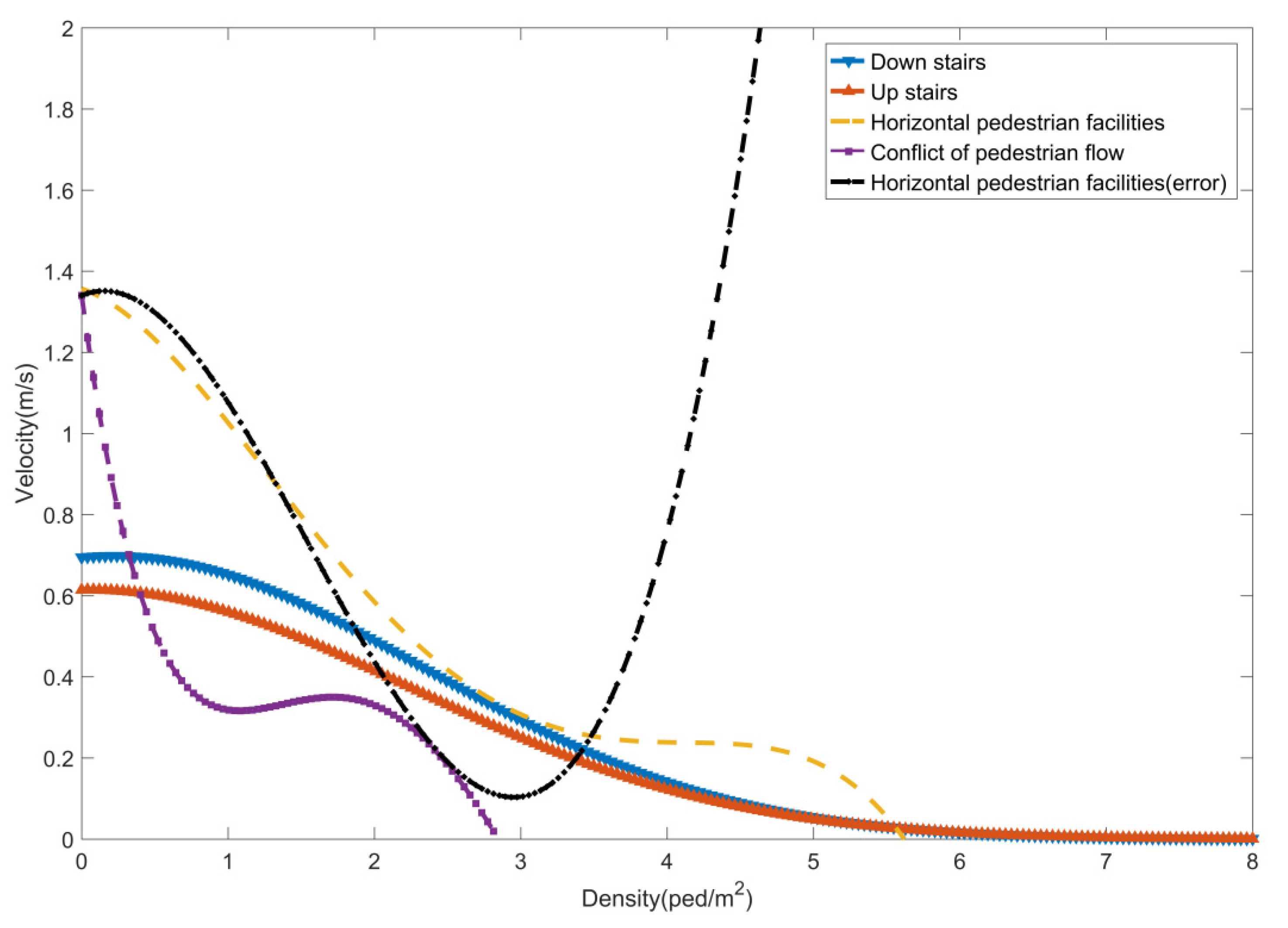
Figure 7.
Simulation Description.
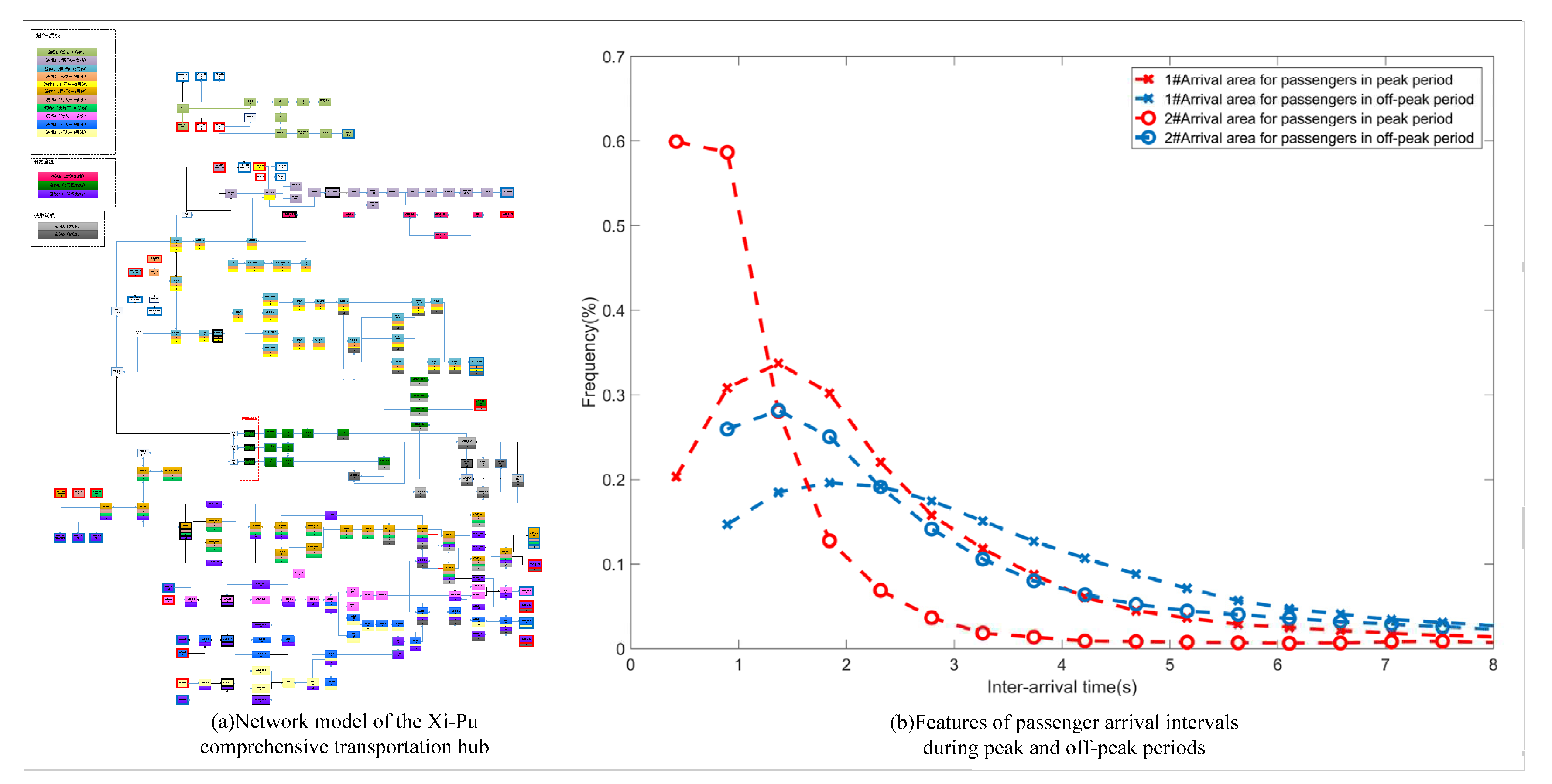
Figure 8.
Simulation results during off-peak periods.
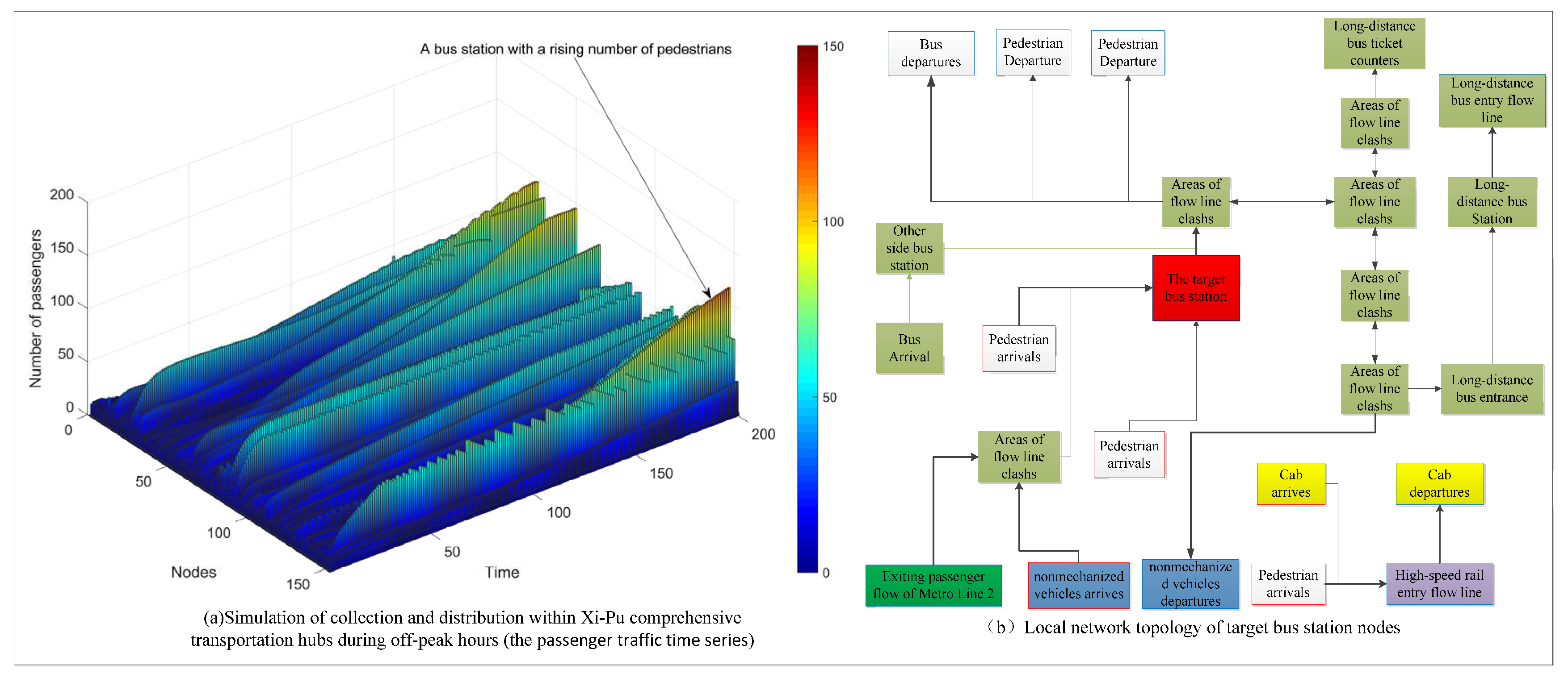
Figure 9.
Analysis of reasons for passenger detention.
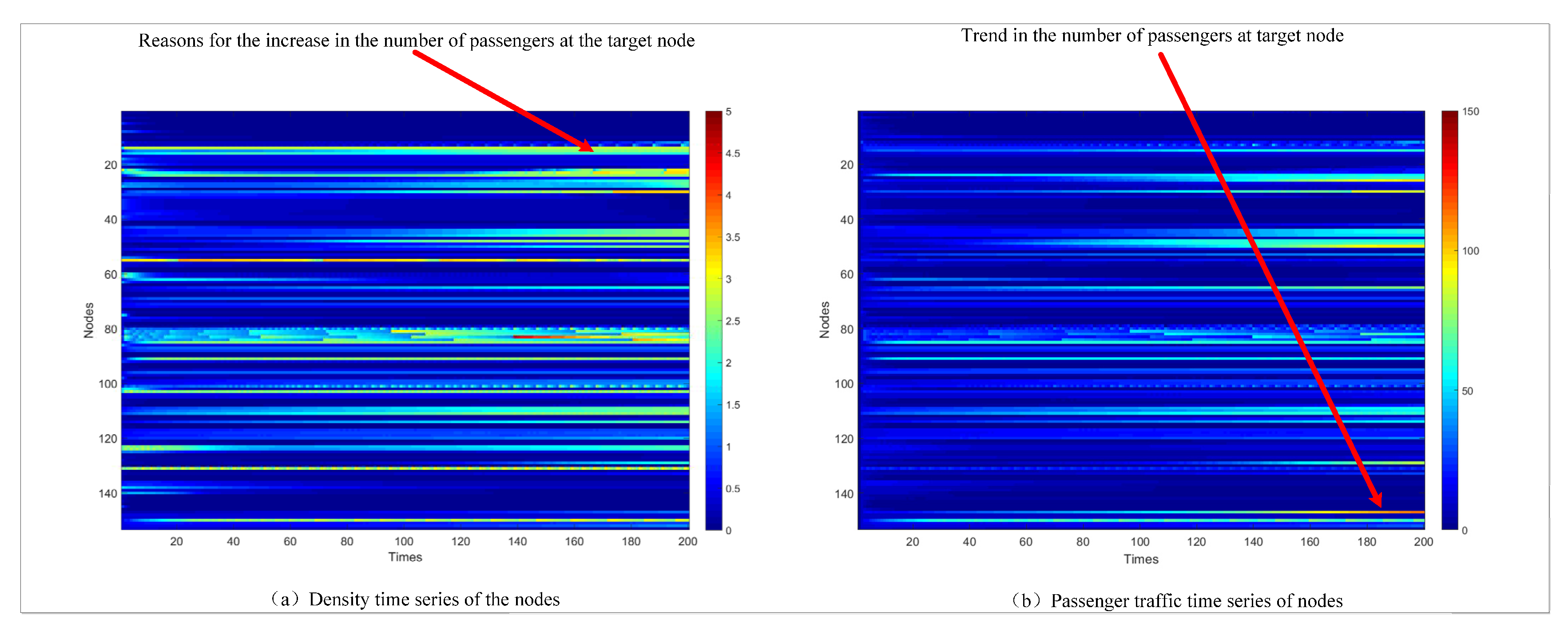
Figure 10.
Simulation results after optimization for node 15 (off-peak period).
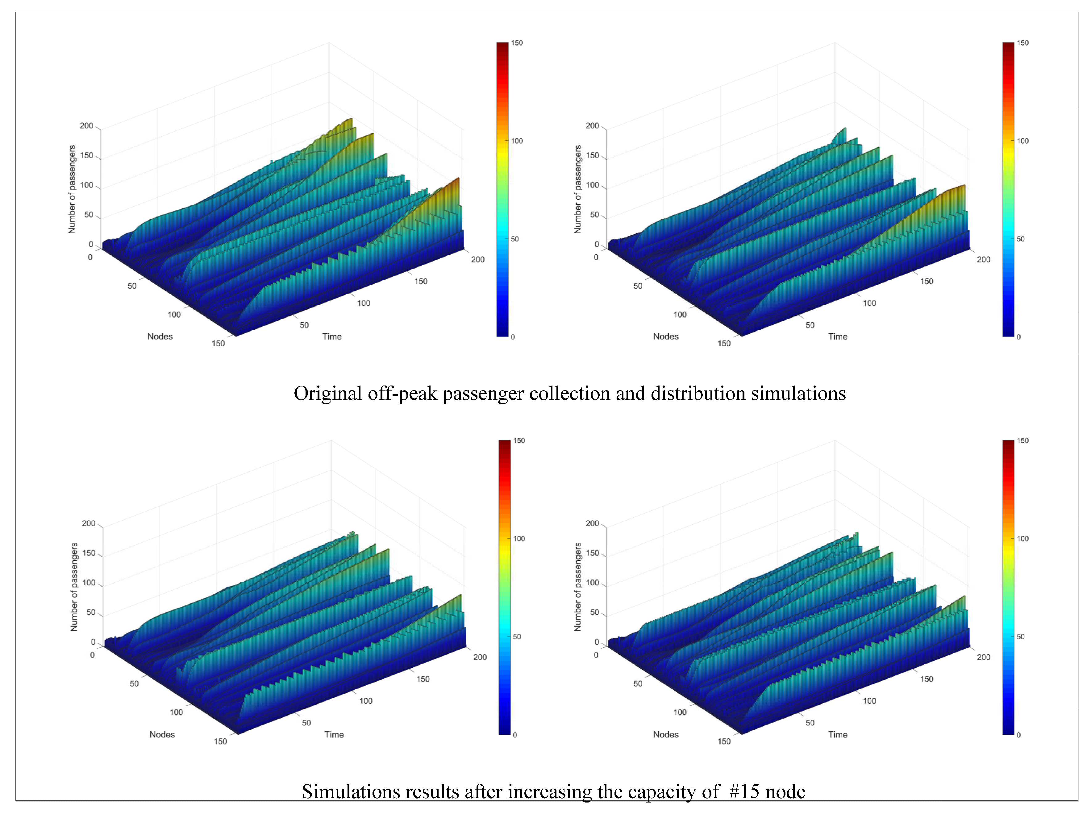
Figure 11.
Simulation results of peak period.
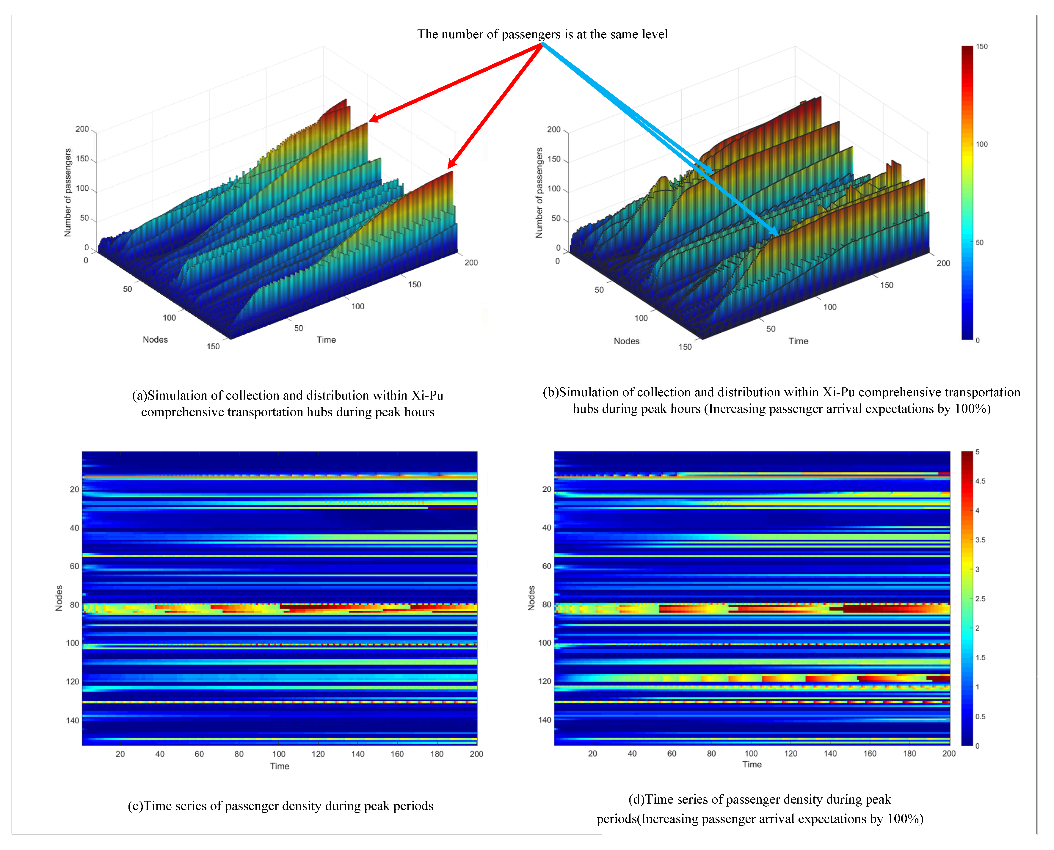
Figure 12.
Passenger flow control scheme based on optimal control theory.

Figure 13.
Optimization Results.
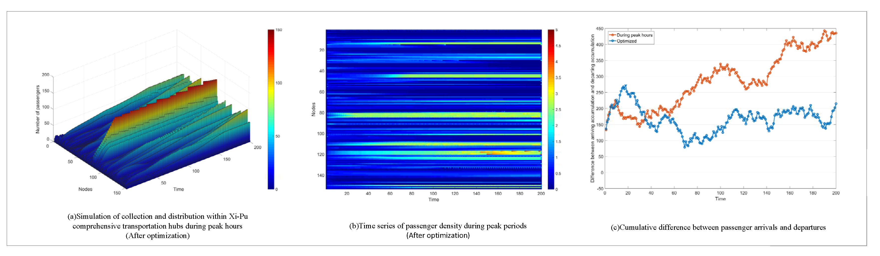

Table 1.
Design of data structure for hub station network model.
| data classification | Description | S | V | ||
|---|---|---|---|---|---|
| ND dynamic |
Load | Automatic pedestrian facilities | occupancy | ✓ | |
| service facility | |||||
| pedestrian facilities | density | ||||
| operational efficiency | Automatic pedestrian facilities | operating speed | × | ||
| service facility | average service time | ||||
| pedestrian facilities | average speed | ||||
| traffic capacity | Automatic pedestrian facilities | capacity | ✓ | ||
| service facility | service efficiency | ||||
| pedestrian facilities | pedestrian flow rate | ||||
| passenger flow | Real-time passenger flow in the node | ✓ | |||
| ED dynamic |
passenger choice behavior | Preference for empty areas for passengers | w1 | × | |
| Status of sink nodes | Whether the sink node is in the inflow failure state | w3 | × | ||
| traffic control measures | current limiting control | w2 | × | ||
| ND static |
Area of the facility | s | × | ||
| Width of the facility | width | × | |||
| Index of transportation process | type1 | × | |||
| pedestrian facilities: 1 ;Automatic pedestrian facilities: 2; service facility:3 |
type2 | × | |||
| Horizontal direction:1;upward direction:2; downward direction:3 | type3 | × | |||
Table 2.
The key issues for MDPM to address.
| Description | Solutions | |
|---|---|---|
| Static heterogeneous | Nodes with different service modes and up/down directions need to be distinguished. | MDPM completes the judgment of the node cases by type2 and type3, and then matches them to the corresponding branches of the fundamental diagram. |
| Dynamic heterogeneous | The heterogeneous pedestrian flow needs to be classified in real time, and the transportation process constraints satisfied by the passenger flow propagation need to be considered. | The transport process constraints are designed as propagation rules for MDPM, while the corresponding branches are added to the fundamental diagram calculation logic. |
| Transportation process constraints | ||
| Network update method | Based on the assumption of the FIFO case, the proposed method eliminates the effect of the update order on the simulation results. | Using an iterative approach, assuming a limited change in node traffic in the short term, the static data from the last cycle is used to calculate the change in traffic for the next cycle |
Table 3.
Density-velocity pedestrian flow fundamental diagram.
| Condition | velocity-density relations | |
| Up stairs[8] | (2) | |
| Down stairs[8] | (3) | |
| Conflict of pedestrian flow[28] | (4) | |
| Horizontal pedestrian facilities[7] | (5) |
Table 4.
Partitioning of Passenger Flow Control Nodes.
| Control Area 1 | Congestion Area 2 | Relief Area 3 |
|---|---|---|
| 10,28,27,128,147 | 15,16,129 | 13,14,26,30,50,141 |
Disclaimer/Publisher’s Note: The statements, opinions and data contained in all publications are solely those of the individual author(s) and contributor(s) and not of MDPI and/or the editor(s). MDPI and/or the editor(s) disclaim responsibility for any injury to people or property resulting from any ideas, methods, instructions or products referred to in the content. |
© 2023 by the authors. Licensee MDPI, Basel, Switzerland. This article is an open access article distributed under the terms and conditions of the Creative Commons Attribution (CC BY) license (http://creativecommons.org/licenses/by/4.0/).
Copyright: This open access article is published under a Creative Commons CC BY 4.0 license, which permit the free download, distribution, and reuse, provided that the author and preprint are cited in any reuse.


