
Submitted:
19 July 2023
Posted:
21 July 2023
You are already at the latest version
Abstract
Conducted within the scope of geochemical exploration in Eastern Thailand, this study aims to detect geochemical anomalies and potential mineral deposits. The objective was to interpret intricate spatial dispersion patterns and concentration levels of deposit pathfinder elements, specifically arsenic (As), copper (Cu), and zinc (Zn), using a comprehensive array of stream sediment geochemistry data. Methodologies involved integrating multifractal properties and traditional statistics, facilitated by the GeoDAS and ArcGIS platforms as instrumental analytical tools. In total, 5,376 stream sediment samples were collected and evaluated, leading to the development of an in-depth geochemical map. The results indicated distinct geological units marked by substantially elevated average values of the aforementioned elements. Identification of geochemical anomalies was achieved through the spatial distribution method and the subsequent application of the Spectrum-Area (S-A) multifractal model. An intriguing link was found between high As concentrations and gold deposits in the area, suggesting As as a viable pathfinder element for gold mineralization. The anomaly maps, generated from the stream sediment data, spotlighted potential zones of interest, offering valuable guidance for future mineral exploration and geological inquiries. Nonetheless, it is vital to recognize that the increased values noted in these maps may be influenced by regional geological factors, emphasizing the necessity for a diverse set of analytical methods for accurate interpretation. The study's significance lies in its pioneering use of the S-A multifractal model in geochemical data analysis. This innovative approach has deepened our comprehension of geochemical dispersion patterns and improved the precision of mineral exploration.
Keywords:
eastern Thailand
; geochemical exploration
; pathfinder elements
; stream sediment
; Spectrum-Area (S-A) multifractal model
1. Introduction
Geochemical exploration is essential in identifying undiscovered mineral deposits [1,2,3,4]. It uses multiple methods to analyze data, revealing the geographic patterns of geochemical markers, identifying related elements, and detecting geochemical anomalies due to mineralization processes [5,6,7]. To investigate these processes, a regional geochemical survey is needed. Regional geochemical surveys are crucial in both environmental and mineral exploration studies [8,9,10]. They provide baseline data about the distribution and abundance of elements and compounds in a region, serving as a reference point for future studies. In environmental studies, these surveys help assess environmental quality, monitor changes over time, and evaluate the effectiveness of mitigation measures [11]. In mineral exploration, they identify areas with economically valuable minerals by creating geochemical maps that highlight anomalous zones [12]. Overall, regional geochemical surveys provide essential information for understanding the environment, identifying mineral deposits, refining geological models, and making informed decisions about land use. These surveys also contribute to geologic mapping efforts and aid in land use planning and resource management. Geochemical anomalies have become more significant in the process of regional mineral prediction in recent decades. Geochemical element distribution patterns at the surface are the result of several primary and secondary geological processes [13,14].
In recent decades, there have been significant advancements in the processing of geochemical data, revolutionizing our understanding of Earth’s processes, environmental changes, and resource assessments. This process involves several crucial steps, including data quality control, normalization, transformation, statistical analysis, visualization, geostatistics, data integration, and computational modeling. Through these methods, data reliability is ensured, enabling effective comparison, interpretation, exploration of relationships and trends, visualization of results, analysis of spatial patterns, integration of data from multiple sources, and simulation of geochemical processes. Researchers have extensively studied state-of-the-art methods for processing geochemical exploration data over the past several decades [15]. The field has witnessed the introduction of various advanced mathematical and statistical techniques to analyze geochemical data exploration [16,17]. These methods have transitioned from traditional and multivariate statistics to more sophisticated approaches like fractal/multifractal models [18,19]and machine learning/deep learning [7]. Geochemistry relies on conventional statistical methods to decipher and interpret the properties of geochemical elements. Traditional statistics, such as classical statistics, have been instrumental in identifying geochemical anomalies using various methods [20,21,22,23,24]. Several successful traditional techniques have been applied to analyze geochemical data. While traditional methods, including multivariate statistics, are commonly employed to define thresholds and distinguish subpopulations [23,25], they often overlook the spatial information and autocorrelation structure present in geochemical data. These methods can be seen as non-spatial statistical tools. To address this limitation, spatial statistical methods, such as the moving average technique, have been developed to incorporate the spatial aspect of geochemical data analysis.
Univariate statistics have become standard in understanding the distribution attributes of geochemical elements, assisting in pinpointing pathfinder elements, and interpreting their dynamics. Meanwhile, spatial data analysis methods, such as geostatistics [26] and fractal analysis [27], have gained popularity as frequency-space-based approaches. These methods, often augmented with Geographic Information Systems (GIS), facilitate the modeling and quantification of spatial discrepancies in geochemical data. Important concepts in non-linear and complexity sciences, fractal and multifractal have found recognition in geosciences [18,26,27,28,29,30] and developed for analyzing geochemical data. These models serve as potent tools in identifying geochemical anomalies and setting geochemical baselines in diverse studies such as concentration-area (C-A) [31,32], spectrum-area model (S-A) [33,34,35], singularity analysis [3,36,37,38].
In this study, the utilization of classical statistics and multifractal properties in analyzing stream sediment geochemistry data for the region. The aim is to distinguish local anomalies from the complex geological background and summarized them to generate a geochemical map. The map provides insights into the concentration values of deposit pathfinder elements, which have multiple chemical element populations and complex spatial dispersion patterns. The primary focus lies in applying advanced GIS techniques [19,39], specifically utilizing the GeoDAS and ArcGIS platforms, to delineate promising areas with anomalies of pathfinder elements [40,41,42,43,44,45,46,47] associated with gold (As, Cu, and Zn) in eastern Thailand.
2. Geological Settings
The study area is located in the eastern region of Thailand. As illustrated in Figure 1, eastern Thailand has a varied topography, with numerous low-relief areas interrupted by linear hills and ridges. Cenozoic strike-slip faults have influenced these landforms to trend NW-SE [48]. The area is characterized by a series of sedimentary basins, volcanic rocks, and granitic intrusions that record a complex tectonic history [49] involving the Sibumasu terrane, Chanthaburi terrane, and Indochina terrane [50,51,52]. During the Permo-Triassic period, a volcanic arc system [53] existed in the Chanthaburi terrane, which is characterized by its location, sandwiched between the Indochina and Sibumasu continental blocks.
The Chanthaburi terrane is a distinct fragment of the Sukhothai Arc, as identified by Sone and Metcalfe in 2008. Noted for its I-type granitic plutons and radiometrically linked to the Triassic-Jurassic eras, the terrane is defined by its boundaries with the Indochina and Sibumasu blocks, outlined by the Sa Kaeo Suture [54] and the Klaeng tectonic line respectively. This terrane is home to a diverse range of marine sediments from the Carboniferous and late Permian-Triassic periods, all with rich fossil records, as well as deep-water Triassic sediments and younger Mesozoic continental sediments [55,56,57,58]. Additionally, the Klaeng tectonic line, a significant fault, speaks to a past of tectonic activity and collision between the Sibumasu block and the southern Sukhothai Arc. This fault line exhibits several geological characteristics, including mylonitic gneisses and low-grade metamorphic rocks [59].
The Chanthaburi terrane also includes various sedimentary deposits. Carboniferous sediments found in three major limestone hills exhibit similarities with Early Carboniferous fauna found in other parts of Thailand and Laos. The terrane also houses late Permian-Triassic sediments, particularly those discovered in the Sukpaiwan Formation. These deposits contain a diverse range of fossils that establish a stratigraphic continuity from the late Permian to the Middle Triassic [57,59]. The terrane also contains Triassic sediments from deeper marine environments, as represented by the Pong Nam Ron Formation and the Noen Po Formation, inclusive of cherts from the Late and Middle Triassic [60,61,62]. Furthermore, it hosts younger Mesozoic continental sediments, conspicuous in southeast Thailand, which have been connected to the Jurassic-Cretaceous Khorat Group [63,64,65,66,67].
Base on the granitic belt in Thailand is composed of the Western, Central, and Eastern belts [68], as shown in Figure 2. Eastern Thailand incorporates the Triassic granite found in the Central belt, referred to as the Sibumasu terrane. This type of terrane is classified as S-type granite. Additionally, the Chanthaburi terrane, classified as I-type granite, is known as the Triassic granite in the Eastern belt. Notably, gold deposits are related to the I-type granite found in the Chanthaburi Terrane [60,69] while heavy minerals are associated with the S-type granite [69,70,71].
This area has several significant mineral deposits, which align with the Central metallogenic province [69]. Some base metals including chromium, tungsten, gold, silver, and copper [72], these minerals are primarily found in association with Permo-Triassic volcanic rocks and Triassic granitic intrusions, which are believed to have been emplaced during the collision of the Indian and Eurasian Plates [73]. Also found gemstones and silica sand deposits are present in the east corner of the country, and recent exploration has also shown that gold potential is also high [74]. Finally, in the Gulf of Thailand, numerous Tertiary basins are the source of natural gas and petroleum (Figure 2).
3. Geochemical Data
The total collected samples were 5,376 stream sediment samples (Figure 3) from stream systems in eastern Thailand, with a density of a sample per 5 km2. The data were collected under the Department of Mineral Resources in Thailand (DMR), covering 34,380 km2 of territory with multi-element analyses of 12 elements, with elements As (arsenic), Ba (barium), Co (cobalt), Cr (chromium), Cu (copper), Fe [75], Mg (magnesium), Mn (manganese), Ni (nickel), Pb (lead), V (vanadium), and Zn (zinc). The samples were collected from active stream sediment [76] consisting of clay to sand-sized particles along a 30-50 m stretch of the stream. The sediment sample was prepared by sieving it to provide 2-3 kg of the 80-mesh fraction for analysis. Large samples were necessary to minimize the “nugget effect,” which refers to small-scale variations in the element concentration within a sample. A multi-element analytical methodology and a unified data quality monitoring the procedure was used to analyze the sediment samples, each sample was digested in a modified aqua regia solution and analyzed by inductively coupled plasma optical emission spectrometry (ICP-OES) analysis [77] for 12 elements with numbers in parentheses denoting detection limits: As (2 ppm), Ba (3 ppm), Co (1 ppm), Cr (1 ppm), Cu (2 ppm), Fe (30 ppm), Mg (50 ppm), Mn (1 ppm), Ni (1 ppm), Pb (4 ppm), V (1 ppm), and Zn (7 ppm).
4. Methodology
4.1. Descriptive Statistics
Various measures are used in statistical analysis, including the maximum value (Max), minimum value (Min), average value, mean value (X), standard deviation (SD), and coefficient of variation (CV). These measures are essential for understanding the behavior of geochemical elements in the study area and comparing datasets. A high SD indicates that the data points are widely spread out from the mean, while a low SD indicates that the data points are tightly clustered around the mean. The SD is useful for comparing the variability of two or more datasets or determining whether a particular data point is statistically significant or unusual relative to the rest of the data [78]. Elements concentrations within these samples are considered because these elements represent the mineralization composition in this region [33].
4.2. The Spectrum-Area (S-A) Multifractal Model
The S-A model was developed by Cheng et al. in 1999, 2012 and is a helpful method for identifying mixed geochemical patterns in complex geological environments. This model separates geochemical anomalies from the background based on distinct anisotropic scaling properties in the frequency domain, which has been a powerful tool to decompose mixed geochemical patterns [31,79]. The S-A model employs spectral analysis. The spatial distribution of orebodies can be better understood using these novel models. To create a new method that can not only distinguish between anomalies and background but also reveal information on the anisotropic scale invariance of geochemical patterns, Cao and Cheng (2012) merged the S-A model and generalized scale invariance. Using a power-law function that describes the relationship between the spectral energy density value (S) and the area in units (A) of the wave number with a threshold above (≥S) with spectral energy density values above S on the power density plane [80].
The equation of the S-A model:
A (≥S) α S-2d/β
Where S is the spectral energy density value, A (≥S) is the area with a threshold larger than or equal to S, β is an anisotropic scaling exponent, d is a parameter representing the degree of overall concentration, and ∝ denotes proportionality.
The following are the steps for applying the S-A model: (1) To turn the gridded data into the frequency domain, use the fast Fourier transformation. (2) Establish the power spectrum of the data. (3) Compute A(S) to find the region with a threshold greater than or equal to S. (4) Make an S-A log-log plot. (5) Before creating the filter, choose the S threshold value (breakpoints in the log-log plot). (6) An inverse fast Fourier technique is used to transform the resulting power spectra. In step 5, there can be two filters. The low- and high-pass filters result in the creation of two maps, the first of which is the anomaly map and the second of which is the background map.
5. Result and Discussion
5.1. Descriptive Statistics
Descriptive statistics of pathfinder elements for gold deposits (As, Cu, and Zn) are shown in Table 1. High coefficients of variation (CV) values for As, Cu, and Zn concentration (183.61%, 159.75%, and 302.55% respectively) indicate the extremely variable concentrations of these elements. The CV values were used for the description of global variability. These statistical findings suggest that eastern Thailand comprises a variety of geochemical environments and has undergone a variety of different geological events over geological time that resulted in complex oreforming processes. Some of the values, particularly the incredibly high values, might fit fractal or multifractal distributions. Afterward, based on SPSS and using the fractal distribution histograms and a quantile-quantile (Q-Q) plot for visualizing the distribution of geochemical data. The distribution histograms (log 10) 4 elements of As, Cu, and Zn have high skewness values, indicating that these data are not normally distributed and contain outliers and show clearly positively skewed distributions indicating that the majority of the data points are concentrated toward the low of the distribution. The skewness of As, Cu, and Zn are 16.74, 31.25, and 6.86 respectively. Based on their Q-Q plots indicate that were not normally distributed [2] because the point dots depart from the normal straight lines (Figure 4).
5.2. Spatial Distribution of As, Cu, and Zn
Anomaly areas with high stream sediment As concentrations (>24.00 ppm, 95th percentile), represented by red shading, are delineated in Figure 5. In total, anomalous can be divided into three zones in NW-SE orientations. The first zone (I) is located in the western of the study area part of the Sibumasu Terrane underlain mostly by Quaternary sediment (Q) and is associated with Granitic rocks (Trgr) and the sedimentary rocks Carboniferous-Permian (CP). The second zone (II) is located in the middle of the study area part of Chanthaburi Terrane and is associated with the granitic rocks (Trgr) intrusion in the sedimentary rocks Permian (PE), Upper Carboniferous (C2), Permian-Triassic mixed marine (PTr), Triassic Noen Phuyaiyeu formation (Trn), and Jurassic-Cretaceous Khorat group (JK). The third zone (III) represents the eastern part of the study area including the Chanthaburi Terrane and Indochina Terrane associated with the Granitic rocks (Trgr), Permian-Triassic volcanic rock (PTrv), and the sedimentary rocks Early-Middle Permian limestone Sa Kaeo Suture melange (Ps-2).
High stream sediment anomaly zones In Figure 5, Cu concentrations (>50.50 ppm, 95th percentile) are indicated by red shading. Anomaly can be split into three zones overall in NW-SE orientations. The first zone (I) is located in the western part of Sibumasu Terrane and is associated with Granitic rocks (Trgr) and the sedimentary rocks Carboniferous-Permian (CP). The second zone (II) is located in the middle of the study area part of Chanthaburi Terrane and is associated with the sedimentary rocks Permian (PE) The third zone (III) is located in the eastern of the study area part of the Indochina Terrane associated with the Intrusive rocks Permian volcanic [81].
Anomaly regions with high stream sediment Zn (Figure 5) contents (>100 ppm, 95th percentile) are indicated by red stippling. In total, anomalous can be divided into one zones (I) in NW-SE orientations is located in the western part of Sibumasu Terrane and is associated with Granitic rocks (Trgr) and the sedimentary rocks Permian (PE), and Carboniferous-Permian (CP). The second zone (II) is located in the middle of the study area part of Chanthaburi Terrane underlain mostly by Quaternary sediment (Q).
The elements were distributed statistically across the geological units, including Quaternary (Q), Cretaceous Sau Khua formation (Ksk), Jurassic-Cretaceous Khorat group (JK), Jurassic-Cretaceous Lam Thup formation (JKl), Jurassic-Cretaceous Phra Wihan formation (JKpw), Jurassic Phu Kradung formation (Jpk), Triassic Pong Nam Ron formation (Trpn), Triassic Noen Phuyaiyeu formation (Trn), Permian-Triassic mixed marine (PTr), Early-Middle Permian limestone Sa Kaeo Suture melange (Ps-2), Early-Middle Permian limestone (Ps-1), Early-Middle Permian Saraburi group [54], Carboniferous-Permian (CP), Upper Carboniferous (C2), Lower Carboniferous (C1), Devonian- Carboniferous (DC), Silurian-Devonian (SD), Permian (PE), Basalt deposits (Qbs), Granitic rock (Trgr), Permian-Triassic volcanic (PTru, PTrv), and Permian volcanic [81]. Table 2 summarizes these units, and their distribution characteristics were analyzed to determine the distribution of elements.
The average value (X) of As element in Upper Carboniferous (C2), Permian-Triassic mixed marine (PTr), Early-Middle Permian limestone Sa Kaeo Suture melange (Ps-2) (22.33, 19.74, and 19.74 respectively) are higher than the average value of the whole unit but the coefficient (Cv) are low showing weak activity and strong stability. The coefficient of variation (Cv) in Permian (PE), Jurassic Phu Kradung formation (Jpk), and Early-Middle Permian limestone (Ps-1) are 1.84, 1.82, and 1.78 respectively and the Quaternary (Q), in the eastern part is the highest value of 2.15, which shows that the active migration ability of As element is strong.
Average value (X) of Cu element in Permian volcanic [81], Permian-Triassic volcanic (PTru, PTrv), Early-Middle Permian limestone Sa Kaeo Suture melange (Ps-2), and Devonian- Carboniferous (DC), (108.50, 41.54, 31.12 and 30.39 respectively) are higher than the average value of the whole unit and the coefficient (Cv) of are low and Permian volcanic [81] is lowest showing very weak activity and strong stability. The coefficient of variation (Cv) in Permian (PE) and Silurian-Devonian (SD), are 1.60 and 1.12 respectively and the Quaternary (Q), in the eastern part is the highest value of 2.63, which shows that the active migration ability of Cu element is strong.
Zn element’s average value (X) in Permian volcanic [81], Basalt deposits (Qbs), and the Quaternary (Q) (69.83, 61.04, and 57.38 respectively) are higher than the average value of the whole unit and the coefficient (Cv) of are low and Permian volcanic [81] is lowest showing very weak activity and strong stability. The coefficient of variation (Cv) in the Quaternary (Q) and Permian (PE) are 3.60 and 3.03 respectively and which shows that the active migration ability of the Zn element is strong.
The elements were distributed statistically across the geological units, including Quaternary (Q), Cretaceous Sau Khua formation (Ksk), Jurassic-Cretaceous Khorat group (JK), Jurassic-Cretaceous Lam Thup formation (JKl), Jurassic-Cretaceous Phra Wihan formation (JKpw), Jurassic Phu Kradung formation (Jpk), Triassic Pong Nam Ron formation (Trpn), Triassic Noen Phuyaiyeu formation (Trn), Permian-Triassic mixed marine (PTr), Early-Middle Permian limestone Sa Kaeo Suture melange (Ps-2), Early-Middle Permian limestone (Ps-1), Early-Middle Permian Saraburi group [54], Carboniferous-Permian (CP), Upper Carboniferous (C2), Lower Carboniferous (C1), Devonian- Carboniferous (DC), Silurian-Devonian (SD), Permian (PE), Basalt deposits (Qbs), Granitic rock (Trgr), Permian-Triassic volcanic (PTru, PTrv), and Permian volcanic [81] [81]. Table 2 summarizes these units, and their distribution characteristics were analyzed to determine the distribution of elements.
The average value (X) of As element in Upper Carboniferous (C2), Permian-Triassic mixed marine (PTr), Early-Middle Permian limestone Sa Kaeo Suture melange (Ps-2) (22.33, 19.74, and 19.74 respectively) are higher than the average value of the whole unit but the coefficient (Cv) are low showing weak activity and strong stability. The coefficient of variation (Cv) in Permian (PE), Jurassic Phu Kradung formation (Jpk), and Early-Middle Permian limestone (Ps-1) are 1.84, 1.82, and 1.78 respectively and the Quaternary (Q), in the eastern part is the highest value of 2.15, which shows that the active migration ability of As element is strong.
Average value (X) of Cu element in Permian volcanic [81], Permian-Triassic volcanic (PTru, PTrv), Early-Middle Permian limestone Sa Kaeo Suture melange (Ps-2), and Devonian- Carboniferous (DC), (108.50, 41.54, 31.12 and 30.39 respectively) are higher than the average value of the whole unit and the coefficient (Cv) of are low and Permian volcanic [81] is lowest showing very weak activity and strong stability. The coefficient of variation (Cv) in Permian (PE) and Silurian-Devonian (SD), are 1.60 and 1.12 respectively and the Quaternary (Q), in the eastern part is the highest value of 2.63, which shows that the active migration ability of Cu element is strong.
Zn element’s average value (X) in Permian volcanic [81], Basalt deposits (Qbs), and the Quaternary (Q) (69.83, 61.04, and 57.38 respectively) are higher than the average value of the whole unit and the coefficient (Cv) of are low and Permian volcanic [81] is lowest showing very weak activity and strong stability. The coefficient of variation (Cv) in the Quaternary (Q) and Permian (PE) are 3.60 and 3.03 respectively and which shows that the active migration ability of the Zn element is strong.
5.3. Determining Thresholds Using the S-A Model
The decomposed geochemical maps were produced by IDW using the S-A method, which was applied to each raster map: anomalies and backgrounds of the distributions for As, Cu, and Zn were built up using the inverse distance weighting (IDW) interpolation method [82] by ArcGIS software (Figure 6). One of the most widely used moving-average interpolation methods is IDW, which works under the concept that within observations’ values have more effect on interpolated values than distant observations’ values. The IDW approach has the benefit of being easy to use and understand, and it is also simple to apply. The main issue is from the weights being determined solely based on location and ignoring the variance of the results [83]. The failure to take into account the local features of data is a typical flaw in moving average interpolation techniques like IDW. Then, the power spectrum densities (S) were calculated for the elemental distributions. The S-A multifractal model was used to decompose complex geochemical patterns into constituent anomalous and background patterns [82] and was implemented with the aid of GeoDAS software [34]. The power spectrum density (S) and the area (A) that is greater than or equal to S could be fitted with two straight lines using the least square method.
The S-A plot consisting of S versus the number of cells greater than or equal to S could be fitted by three straight lines using the least square method. The left lines of the cutoff values represented the geochemical noise, anomaly, and background, respectively. Then these three components were converted to the spatial domain by an inverse Fourier transformation. The decomposed maps show the spatial distribution of the geochemical anomaly and the geochemical background of As, Cu, and Zn.
Using the S-A approach, the geochemical map of As concentration (Figure 6) was divided into two spatial components. The As geochemical map was converted into the frequency domain using a Fourier transform. The relationship between A (≥S) and S is shown on an As log-log scale (Figure 6a). The data can be fitted with three straight-line segments using the Least Squares [84] method. These segments represent three power energy spectrum S ranges, each distinguished by a unique scaling property of the S-A relation. There are three ranges of S: left (S ≤ 4,138), middle (4,138 < S ≤ 20,606), and right (S ≥ 20,606). The last segment displays a short-range spectrum of high frequencies. Two filters were defined using two distinct ranges of S separated by the threshold value S = 20,606: an anomaly filter with S < 20,606 (Figure 6b) and a background filter with S > 20,606 (Figure 6c). These filters are irregularly shaped to preserve the anisotropy and interior structure of the two-dimensional power energy spectrum, which they represent. The two maps are the result of applying the two filters obtained from the S-A plot to the Fourier-transformed functions and then converting them back into the spatial domain.
The geochemical map of Cu concentration (Figure 7) was decomposed into two spatial components using the S-A method. The Cu geochemical map was converted into the frequency domain using a Fourier transform. The relationship between A (≥S) and S is shown on an As log-log scale (Figure 7a). There are three ranges of S: left (S ≤ 3,488), middle (3,488 < S ≤ 114,777), and right (S ≥ 114,777). The last segment displays a short-range spectrum of high frequencies. Two filters were defined using two distinct ranges of S separated by the threshold value S = 114,777: an anomaly filter with S < 114,777 (Figure 7b) and a background filter with S > 114,777 (Figure 7c).
The S-A approach was used to divide the geochemical map of Zn concentration (Figure 8) into two spatial components. Using a Fourier transform, the Zn geochemical map was transformed into the frequency domain. The relationship between A (≥S) and S is shown on an As log-log scale (Figure 8a). There are three ranges of S: left (S ≤ 12,889), middle (12,889 < S ≤ 850,339), and right (S ≥ 850,339). The last segment displays a short-range spectrum of high frequencies. Two filters were defined using two distinct ranges of S separated by the threshold value S = 850,339: an anomaly filter with S < 850,339 (Figure 8b) and a background filter with S > 850,339 (Figure 8c).
The decomposed pattern obtained from the concentration map of arsenic (As) using the background filter reveals variations in As concentration values in the background, which could indicate favorable geological conditions for the occurrence of gold mineralization. Overlaying the known gold deposits on a background map shows that these deposits are located within areas characterized by high background As values found around intrusive and sedimentary rocks in the central (zone II), and eastern parts (zone III). The anomaly map suggests high mineral deposit potential in areas with NW-SE trending faults and mapped intrusions [85]. The most of As anomaly map shows that high values follow around intrusive rocks in the middle zone Chanthaburi terrane and along NW-SE trending fault/fractures, which are favorable areas for mineral deposits. These results of the As element anomaly assessment of pathfinder elements for gold deposits may indicate the potential relationship to the gold deposits in the study area. The integrated anomalies of As occur around the intrusions and in the vicinity of faults in the center. However, the As element anomalies occurring in the western part of the study area are not relative to gold deposits and may be caused by the high background concentration values of the intrusive rock of the Sibumasu terrain, which is divided by the tectonic line NW-SE trend, As element anomaly assessment and pathfinder elements for gold deposits support this potential [86,87], further investigation of gold anomalies around intrusions and faults is recommended.
Similar maps with distinctive features were generated using copper (Cu) and zinc (Zn) data. These two maps are also displayed in Figure 7 and Figure 8, depicting the NE-SW distribution characteristics of the area. Interestingly, the high concentrations observed in the geochemical maps of the study area most of the anomalies do not align with the presence of the known gold deposits in the western part (zone I). Instead, they are primarily distributed in the western part around the intrusive rocks and sedimentary rocks of the Sibumasu terrane. The central (zone II) shows that the anomaly high value follows around the Permian rocks (PE).
6. Conclusions
1. Stream sediment geochemical data analysis provides a robust means to identify potential mineral deposits across a large region. Traditional statistical methods may fail to account for spatial variability in complex geological settings, but incorporating the S-A multifractal model helps to better interpret the data. This approach provides an enhanced understanding of the geological processes, furthering our ability to pinpoint exploration targets. Through statistical analysis, the study uncovers a distinct distribution of elements such as As, Cu, and Zn across various geological units. These findings offer crucial insight into the dynamic interactions of elements within different geological contexts, revealing the migration abilities of these elements in specific units. Overall, the study demonstrates that the S-A multifractal model provides a powerful tool for analyzing stream sediment geochemical data. This approach helps to identify specific geological processes that contribute to patterns in the data, improving the understanding of statistical results and the regularity of changes in these properties in spatial and temporal domains. This information proves valuable in identifying precise exploration targets for mineral deposits.
2. By applying the S-A multifractal model and the Inverse Distance Weighting (IDW) method, the research has successfully decomposed geochemical maps into anomalous and background patterns. The anomaly map for the As element, in particular, has shown a strong correlation with the gold deposits in the study area, indicating its potential as a reliable indicator for identifying gold deposits. While geochemical maps derived from stream sediment data offer an initial understanding of element distribution, it is important to exercise caution during interpretation due to potential influences from regional geological factors.
3. The study has created prediction maps, pinpointing areas of interest associated with pathfinder elements within the gold deposit zones and beyond. These maps can guide mineral exploration by narrowing down target areas for further investigation. It underlines the importance of utilizing a variety of analytical methods for accurate results, acknowledging that regional geological factors can contribute to elevated values unrelated to mineralization.
Author Contributions
Conceptualization, O.Y. and S.X.; methodology, O.Y. and S.X.; software, O.Y., and J.D.; validation, O.Y., S.X. and P.C.; formal analysis, O.Y.; data curation, O.Y. and W.W.; writing—original draft preparation, O.Y.; writing—review and editing, O.Y., S.X. and P.C.; visualization, O.Y. and J.D.; supervision, O.Y. and S.X.; project administration, O.Y.; funding acquisition, O.Y. All authors have read and agreed to the published version of the manuscript.
Funding
This research received no external funding.
Data Availability Statement
Not applicable.
Acknowledgments
The authors would like to express our heartfelt appreciation to the Department of Mineral Resources in Thailand (DMR) for providing the necessary data for this research. We are grateful to the staff and administrators of the Geotechnology Division of DMR for their administrative support and access to resources. Special thanks to Dr.Ratthaphon Amphon and Dr.Jongkonnee Khanmanee for their valuable suggestions. Additionally, we sincerely appreciate all the editors and reviewers who have dedicated their time and expertise to help us improve the manuscript. Their insightful comments and feedback have played a crucial role in shaping the final version of this paper.
Conflicts of Interest
The authors declare no conflict of interest.
References
- Cheng, Q. , Singularity theory and methods for mapping geochemical anomalies caused by buried sources and for predicting undiscovered mineral deposits in covered areas. Journal of Geochemical Exploration 2012, 122, 55–70. [Google Scholar] [CrossRef]
- Zuo, R., Q. Cheng, and Q. Xia, Application of fractal models to characterization of vertical distribution of geochemical element concentration. Journal of Geochemical Exploration 2009, 102, 37–43. [Google Scholar] [CrossRef]
- Cheng, Q. , Mapping singularities with stream sediment geochemical data for prediction of undiscovered mineral deposits in Gejiu, Yunnan Province, China. Ore Geology Reviews 2007, 32, 314–324. [Google Scholar] [CrossRef]
- Parsa, M., A. Maghsoudi, and M. Yousefi, A Receiver Operating Characteristics-Based Geochemical Data Fusion Technique for Targeting Undiscovered Mineral Deposits. Natural Resources Research 2018, 27, 15–28. [Google Scholar] [CrossRef]
- Zuo, R. and Y. Xiong, Geodata science and geochemical mapping. Journal of Geochemical Exploration 2020, 209, 106431. [Google Scholar] [CrossRef]
- Grunsky, E.C. and P.d. Caritat, State-of-the-art analysis of geochemical data for mineral exploration. Geochemistry: Exploration, Environment, Analysis 2020, 20, 217–232. [Google Scholar]
- Zuo, R. , et al., The processing methods of geochemical exploration data: past, present, and future. Applied Geochemistry 2021, 132, 105072. [Google Scholar] [CrossRef]
- Cohen, D. , et al., Major advances in exploration geochemistry, 1998–2007, 2010.
- Winterburn, P.A., R. R. Noble, and D. Lawie, Advances in exploration geochemistry, 2007 to 2017 and beyond. Geochemistry: Exploration, Environment, Analysis 2020, 20, 157–166. [Google Scholar]
- Zuo, R., E. J.M. Carranza, and Q. Cheng, Fractal/multifractal modelling of geochemical exploration data. Journal of Geochemical Exploration 2012, 122, 1–3. [Google Scholar] [CrossRef]
- Xie, S. , et al., Quantitative prediction of potential areas likely to yield Se-rich and Cd-low rice using fuzzy weights-of-evidence method. Science of The Total Environment 2023, 889, 164015. [Google Scholar] [CrossRef]
- Yang, F. , et al., Geochemical quantitative assessment of mineral resource potential in the Da Hinggan Mountains in Inner Mongolia, China. Minerals 2022, 12, 434. [Google Scholar] [CrossRef]
- Cohen, D. and R. Bowell, 13.24-Exploration Geochemistry. Treatise on Geochemistry, 2nd ed.; Holland, HD, Turekian, KK, Eds, 2014, 623-650.
- Xie, S. , et al., Quantitative prediction of prospectivity for Pb–Zn deposits in Guangxi (China) by back-propagation neural network and fuzzy weights-of-evidence modelling. Geochemistry: Exploration, Environment, Analysis 2022, 22, geochem2021–085. [Google Scholar]
- Wang, W., S. Xie, and E.J.M. Carranza, Introduction to the thematic collection: applications of innovations in geochemical data analysis. 2023, The Geological Society of London. p. geochem2022-058. [CrossRef]
- Parsa, M. and E. J.M. Carranza, Modulating the impacts of stochastic uncertainties linked to deposit locations in data-driven predictive mapping of mineral prospectivity. Natural Resources Research 2021, 30, 3081–3097. [Google Scholar]
- Chen, Y., G. Sun, and Q. Zhao, Detection of multivariate geochemical anomalies associated with gold deposits by using distance anomaly factors. Journal of Geochemical exploration 2021, 221, 106704. [Google Scholar] [CrossRef]
- Xie, S. and Z. Bao, Fractal and Multifractal Properties of Geochemical Fields. Mathematical Geology 2004, 36, 847–864. [Google Scholar] [CrossRef]
- Carranza, E.J.M. , Geochemical anomaly and mineral prospectivity mapping in GIS. 2008: Elsevier.
- Harris, D. and G. Pan, Mineral favorability mapping: a comparison of artificial neural networks, logistic regression, and discriminant analysis. Natural Resources Research 1999, 8, 93–109. [Google Scholar] [CrossRef]
- Harris, J., L. Wilkinson, and E. Grunsky, Effective use and interpretation of lithogeochemical data in regional mineral exploration programs: application of Geographic Information Systems (GIS) technology. Ore Geology Reviews 2000, 16, 107–143. [Google Scholar] [CrossRef]
- Hawkes, H. and J. Webb, s., 1962, Geochemistry in mineral exploration. 1962, New York, Harper and Row.
- Sinclair, A. , Selection of threshold values in geochemical data using probability graphs. Journal of geochemical exploration 1974, 3, 129–149. [Google Scholar] [CrossRef]
- Tukey, J.W. , Exploratory data analysis. Vol. 2. 1977: Reading, MA.
- Stanley, C.R. and A.J. Sinclair, Comparison of probability plots and the gap statistic in the selection of thresholds for exploration geochemistry data. journal of Geochemical Exploration 1989, 32, 355–357. [Google Scholar] [CrossRef]
- Matheron, G. , Traité de géostatistique appliquée, Mém BRGM 14. Éditions Technip, Paris, 1962.
- Mandelbrot, B.B. , The fractal geometry of Nature WH Freeman and Company. New York, 1983, 8, 406–406. [Google Scholar]
- Turcotte, D.L. , Fractals in geology and geophysics. Pure and applied Geophysics, 1989, 131, 171–196. [Google Scholar] [CrossRef]
- Cheng, Q. , Multifractality and spatial statistics. Computers & Geosciences 1999, 25, 949–961. [Google Scholar]
- Zhang, Y. , et al., Implication of multifractal analysis for quantitative evaluation of mineral resources in the Central Kunlun area, Xinjiang, China. Geochemistry: Exploration, Environment, Analysis 2022, 22, geochem2021–083. [Google Scholar]
- Cheng, Q., F. P. Agterberg, and S.B. Ballantyne, The separation of geochemical anomalies from background by fractal methods. Journal of Geochemical Exploration 1994, 51, 109–130. [Google Scholar] [CrossRef]
- Behera, S. and M.K. Panigrahi, Mineral prospectivity modelling using singularity mapping and multifractal analysis of stream sediment geochemical data from the auriferous Hutti-Maski schist belt, S. India. Ore Geology Reviews 2021, 131, 104029. [Google Scholar] [CrossRef]
- Cheng, Q. , Spatial and scaling modelling for geochemical anomaly separation. Journal of Geochemical exploration 1999, 65, 175–194. [Google Scholar] [CrossRef]
- Cheng, Q. GeoData Analysis System (GeoDAS) for mineral exploration: User’s guide and exercise manual. in Material for the training workshop on GeoDAS held at York University. 2000.
- Koohzadi, F. , et al., Geochemical exploration for Li in regional scale utilizing Staged Factor Analysis (SFA) and Spectrum-Area (SA) fractal model in north central Iran. Iranian Journal of Earth Sciences 2021, 13, 299–307. [Google Scholar]
- Sadeghi, B. and F. Agterberg, Singularity analysis. Encyclopedia of Mathematical Geosciences 2020, 1–7. [Google Scholar]
- Ali, K., Q. Cheng, and Z. Chen, Multifractal power spectrum and singularity analysis for modelling stream sediment geochemical distribution patterns to identify anomalies related to gold mineralization in Yunnan Province, South China. Geochemistry: Exploration, Environment, Analysis 2007, 7, 293–301. [Google Scholar]
- Cheng, Q. , Multifractal interpolation method for spatial data with singularities. Journal of the Southern African Institute of Mining and Metallurgy 2015, 115, 235–240. [Google Scholar] [CrossRef]
- Zuo, R. and J. Wang, ArcFractal: An ArcGIS add-in for processing geoscience data using fractal/multifractal models. Natural Resources Research 2020, 29, 3–12. [Google Scholar] [CrossRef]
- Song, W. , et al., Genesis, metallogenic model, and prospecting prediction of the Nibao gold deposit in the Guizhou Province, China. Acta Geochimica 2023, 42, 136–152. [Google Scholar] [CrossRef]
- Sunkari, E.D., M. Appiah-Twum, and A. Lermi, Spatial distribution and trace element geochemistry of laterites in Kunche area: Implication for gold exploration targets in NW, Ghana. Journal of African Earth Sciences 2019, 158, 103519. [Google Scholar] [CrossRef]
- Agangi, A. , et al., Antimony in rutile as a pathfinder for orogenic gold deposits. Ore Geology Reviews 2019, 106, 1–11. [Google Scholar] [CrossRef]
- Bayari, E.E., G. Foli, and S.K. Gawu, Geochemical and pathfinder elements assessment in some mineralised regolith profiles in Bole-Nangodi gold belt in north-eastern Ghana. Environmental Earth Sciences 2019, 78, 1–16. [Google Scholar] [CrossRef]
- Arhin, E., S. Boadi, and M.C. Esoah, Identifying pathfinder elements from termite mound samples for gold exploration in regolith complex terrain of the Lawra belt, NW Ghana. Journal of African Earth Sciences 2015, 109, 143–153. [Google Scholar] [CrossRef]
- Anand, R. , et al., Gold and pathfinder elements in ferricrete gold deposits of the Yilgarn Craton of Western Australia: A review with new concepts. Ore Geology Reviews 2019, 104, 294–355. [Google Scholar] [CrossRef]
- Behera, S., M. K. Panigrahi, and A. Pradhan, Identification of geochemical anomaly and gold potential mapping in the Sonakhan Greenstone belt, Central India: An integrated concentration-area fractal and fuzzy AHP approach. Applied Geochemistry 2019, 107, 45–57. [Google Scholar] [CrossRef]
- Mvile, B.N., M. Abu, and J. Kalimenze, Trace elements geochemistry of in situ regolith materials and their implication on gold mineralization and exploration targeting, Dodoma Region, East Africa. Mining, Metallurgy & Exploration 2021, 38, 2075–2087. [Google Scholar]
- Morley, C.K., P. Charusiri, and I.M. Watkinson, Structural geology of Thailand during the Cenozoic. 2011. [CrossRef]
- Ridd, M.F., A.J. Barber, and M.J. Crow, Introduction to the geology of Thailand. 2011.
- Charusiri, P. , Geotectonic evolution of Thailand: a new synthesis. J. Geol. Soc. Thai 2002, 1, 1–20. [Google Scholar]
- Metcalfe, I., C. Henderson, and K. Wakita, Lower Permian conodonts from Palaeo-Tethys ocean plate stratigraphy in the Chiang Mai-Chiang Rai suture zone, northern Thailand. Gondwana Research 2017, 44, 54–66. [Google Scholar] [CrossRef]
- Sone, M., I. Metcalfe, and P. Chaodumrong, The Chanthaburi terrane of southeastern Thailand: Stratigraphic confirmation as a disrupted segment of the Sukhothai Arc. Journal of Asian Earth Sciences 2012, 61, 16–32. [Google Scholar] [CrossRef]
- Hara, H. , et al., Permian–Triassic back-arc basin development in response to Paleo-Tethys subduction, Sa Kaeo–Chanthaburi area in Southeastern Thailand. Gondwana Research 2018, 64, 50–66. [Google Scholar] [CrossRef]
- Saesaengseerung, D. , et al., Discovery of Lower Permian radiolarian and conodont faunas from the bedded chert of the Chanthaburi area along the Sra Kaeo suture zone, eastern Thailand. Paleontological Research 2009, 13, 119–138. [Google Scholar] [CrossRef]
- Fontaine, H. and S. Salyapongse. Unexpected discovery of early Carboniferous (late Visean-Serpukhovian) corals in East Thailand. in Proceedings of the international conference on Stratigraphy and tectonic evolution of Southeast Asia and the South Pacific. 1997.
- Fontaine, H. , et al., Recent biostratigraphic discoveries in Thailand: a preliminary report. CCOP Newsletter 1996, 21, 14–15. [Google Scholar]
- Fontaine, H., S. Salyapongse, and D. Vachard, The Carboniferous of East Thailand—New Information from Microfossils. 1999.
- Sone, M. and I. Metcalfe. Parallel Tethyan sutures and the Sukhothai Island-arc system in Thailand and beyond. in Proceedings of the international symposia on geoscience resources and environments of Asian terranes (GREAT 2008), 4th IGCP. 2008.
- Salyapongse, S. Geology of the Eastern Thailand, Field Excursion Guidebook Route no. 1. in the First International conference on Stratigraphy and Tectonic Evolution of Southeast Asia and the South Pacific. 1997.
- Bunopas, S., Palaeogeographic history of Western Thailand and adjacent parts of Southeast Asia. A plate tectonics interpretation, Geol. Surv. Pap., Dep. Miner. Res. Thailand, 1982.
- Chaodumrong, P., et al. Geology of SW Khorat Plateau and eastern Thailand. in Post-Symposium Excursion Guidebook of Symposium on Geology of Thailand. Department of Mineral Resources Thailand, Bangkok. 2002.
- Chutakositkanon, V. , et al. Tectono-stratigraphy of the Sa Kaeo-Chanthaburi accretionary complex, 4th IGCP. 2008., Eastern Thailand: reconstruction of tectonic evolution of oceanic plate-Indochina collision. in Proceedings of the International Symposia on Geoscience Resources and Environments of Asian Terranes (GREAT 2008). [Google Scholar]
- Crow, M. , Appendix. Radiometric ages of Thailand rocks. The Geology of Thailand. Geological Society, London, 2011, 593-614.
- Palaeozoic–Mesozoic history of SE Asia. Geological Society, London, Special Publications 2011, 355, 7–35.
- DMR, Geologic Map of Thailand 1: 2,500,000: Geological Map of Thailand. 1999, Geological Survey Div., Dept. of Mineral Resources.
- Tansuwan, V. , Geological Map of Changwat Trat 1:250,000. 1997a, Department of Mineral Resources, Thailand, Bangkok.
- Tansuwan, V. , Geology and Mineral Resources Map of Changwat Chanthaburi 1:250,000. 1997b, Department of Mineral Resources Thailand, Bangkok.
- Charusiri, P., et al. Anatomy of Chanthaburi granitoids: geochronology, petrochemistry, tectonics, and associated mineralization. in Proceedings of the National Conference on Geologic Resources of Thailand: Potential for Future Development. Department of Mineral Resources, Ministry of Industry, Bangkok, Thailand. 1992.
- Bunopas, S. and P. Vella. Tectonic and geologic evolution of Thailand. in Proceedings of a workshop on stratigraphic correlation of Thailand and Malaysia. 1983.
- Searle, M. , et al., Tectonic evolution of the Sibumasu–Indochina terrane collision zone in Thailand and Malaysia: constraints from new U–Pb zircon chronology of SE Asian tin granitoids. Journal of the Geological Society 2012, 169, 489–500. [Google Scholar] [CrossRef]
- Cobbing, E. , et al., The granites of the Southeast Asian tin belt. Journal of the Geological Society 1986, 143, 537–550. [Google Scholar] [CrossRef]
- Brown, G.F. , Geologic reconnaissance of the mineral deposits of Thailand. 1951: US Government Printing Office.
- Searle, M.P. and C.K. Morley, Tectonic and thermal evolution of Thailand in the regional context of SE Asia. 2011.
- DMR, Minerals Resources Map of Thailand 1:2,500,00. Bureau of Mineral Resources, Department of Mineral Resources, Thailand, 2006.
- Chen, L. , et al., A multi-convolutional autoencoder approach to multivariate geochemical anomaly recognition. Minerals 2019, 9, 270. [Google Scholar] [CrossRef]
- Xie, S. , et al., Geochemical multifractal distribution patterns in sediments from ordered streams. Geoderma 2010, 160, 36–46. [Google Scholar] [CrossRef]
- Van Loon, J.C. and R. Barefoot, Analytical methods for geochemical exploration. 2013: Elsevier.
- Smith-Forbes, E.V. , et al., Descriptive analysis of common functional limitations identified by patients with shoulder pain. Journal of Sport Rehabilitation 2015, 24, 179–188. [Google Scholar] [CrossRef]
- Xu, Y. and Q. Cheng, A fractal filtering technique for processing regional geochemical maps for mineral exploration. Geochemistry: Exploration, environment, analysis 2001, 1, 147–156. [Google Scholar]
- Zuo, R. and J. Wang, Fractal/multifractal modeling of geochemical data: A review. Journal of Geochemical Exploration 2016, 164, 33–41. [Google Scholar] [CrossRef]
- Darnley, A. , et al., A global geochemical database. Recommendations for international geochemical mapping, 1995.
- Ghezelbash, R., A. Maghsoudi, and M. Daviran, Combination of multifractal geostatistical interpolation and spectrum–area (S–A) fractal model for Cu–Au geochemical prospects in Feizabad district, NE Iran. Arabian Journal of Geosciences 2019, 12, 1–14. [Google Scholar] [CrossRef]
- Xie, X. , et al., Multi-scale geochemical mapping in China. Geochemistry: Exploration, Environment, Analysis 2008, 8, 333–341. [Google Scholar]
- Ke, X. , et al., Multifractal analysis of geochemical stream sediment data in Bange region, northern Tibet. Journal of Earth Science 2015, 26, 317–327. [Google Scholar] [CrossRef]
- Feng, L. , et al., Mapping of geological complexity and analyzing its relationship with the distribution of gold deposits in the Guangxi Gold Ore Province, Southern China. Journal of Geochemical Exploration 2023, 251, 107238. [Google Scholar] [CrossRef]
- Wu, R. , et al., Identifying geochemical anomalies associated with gold mineralization using factor analysis and spectrum–area multifractal model in Laowan District, Qinling-Dabie Metallogenic Belt, Central China. Minerals 2020, 10, 229. [Google Scholar] [CrossRef]
- Farahmandfar, Z. , et al., Description of gold and copper anomalies using fractal and stepwise factor analysis according to stream sediments in NW Iran. Geopersia 2020, 10, 135–148. [Google Scholar]
Figure 1.
Geological map of the study area in eastern Thailand, showing major rock units with the Sakaeo back-arc suture, which encircles the Chanthaburi terrene, and the Klaeng tectonic line, which separates the Chanthaburi and Sibumasu blocks (partly adapted from Chaodumrong, 1992; DMR, 1999; Salyapongse, 1997; Sone et al., 2012).
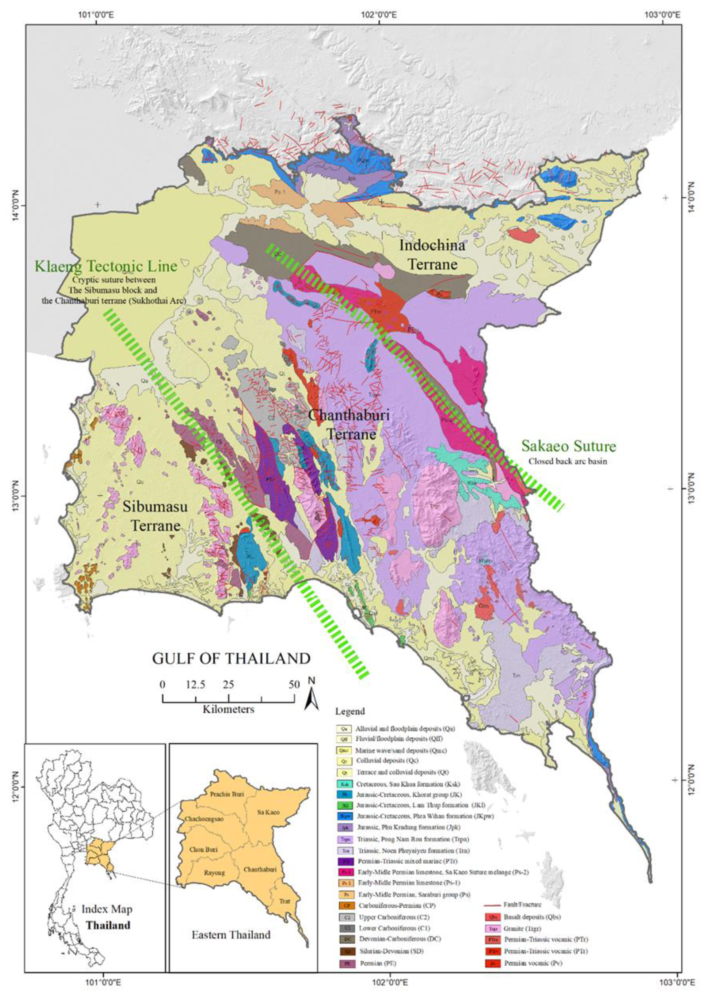
Figure 2.
Mineral deposits in eastern Thailand [74] locates in the Sibumasu Terrane, Chanthaburi Terrane, and Indochina Terrane.
Figure 2.
Mineral deposits in eastern Thailand [74] locates in the Sibumasu Terrane, Chanthaburi Terrane, and Indochina Terrane.
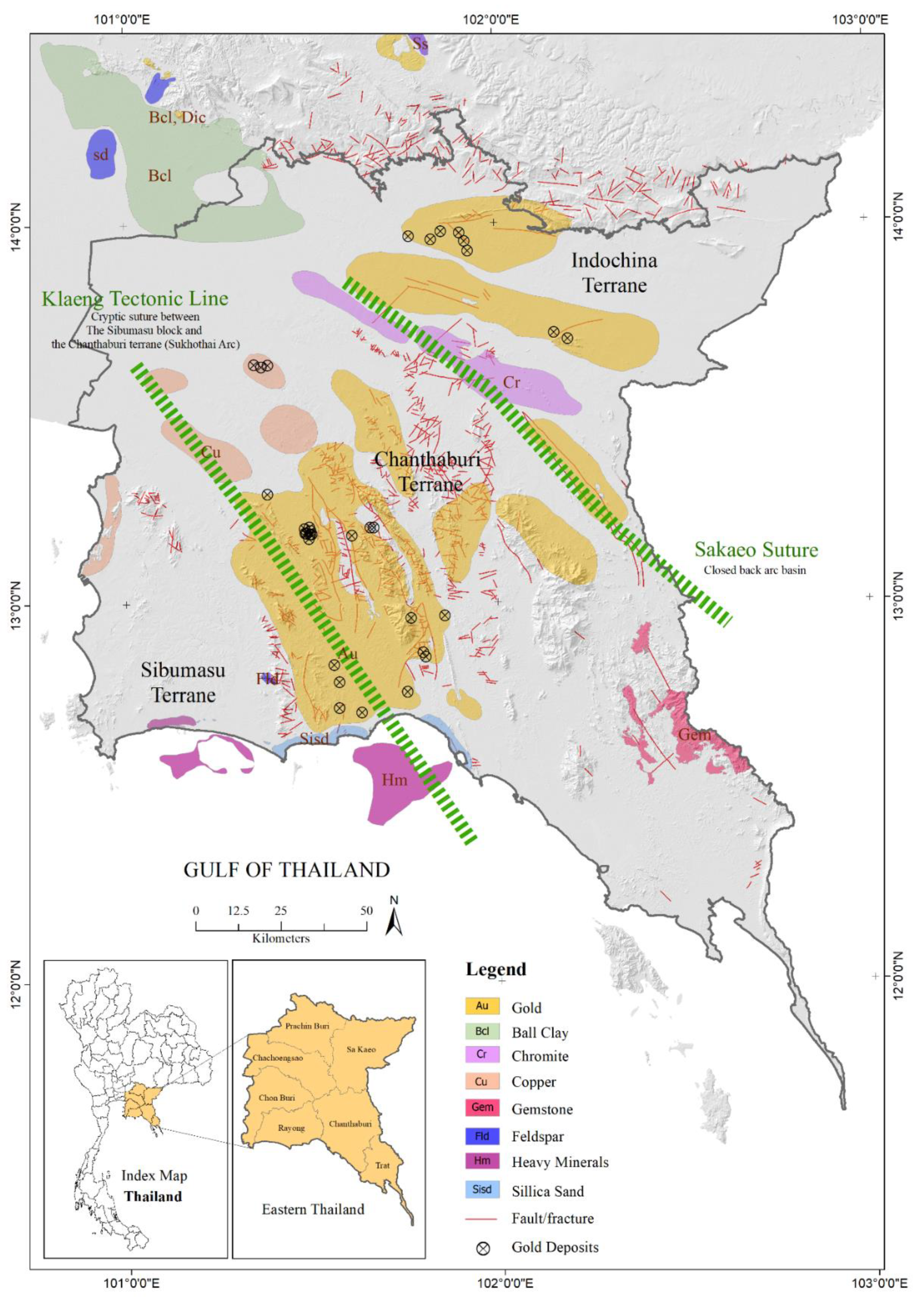
Figure 3.
Mineral deposits in eastern Thailand [74] locates in the Sibumasu Terrane, Chanthaburi Terrane, and Indochina Terrane.
Figure 3.
Mineral deposits in eastern Thailand [74] locates in the Sibumasu Terrane, Chanthaburi Terrane, and Indochina Terrane.
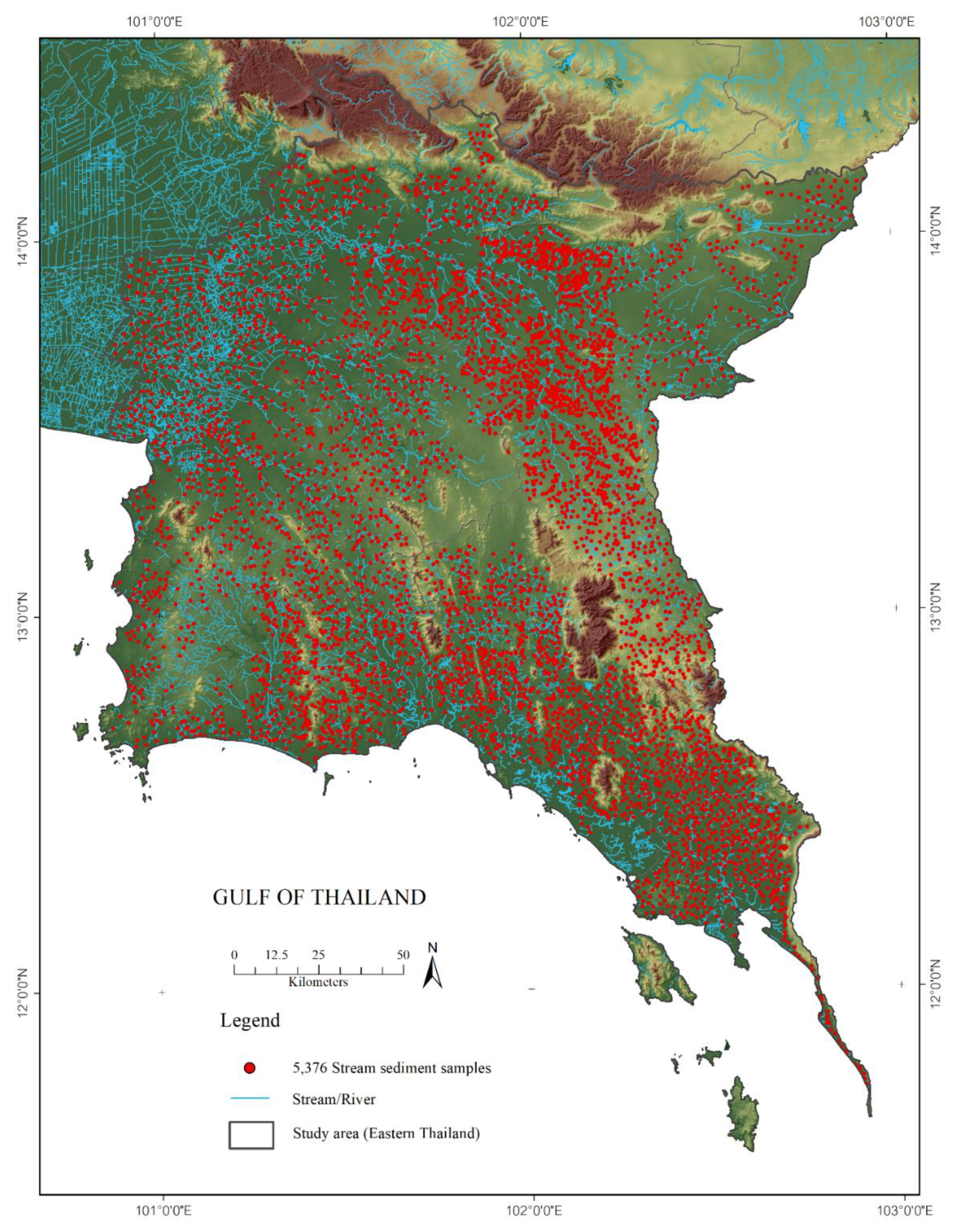
Figure 4.
Distribution histograms of As (a), Cu (c), and Zn (e) concentrations in the stream sediments have high skewness values indicating non-normal distribution, outliers, and positive skewness. Q-Q plots of As (b), Cu (d), and Zn (e) indicate that were not normally distributed.
Figure 4.
Distribution histograms of As (a), Cu (c), and Zn (e) concentrations in the stream sediments have high skewness values indicating non-normal distribution, outliers, and positive skewness. Q-Q plots of As (b), Cu (d), and Zn (e) indicate that were not normally distributed.
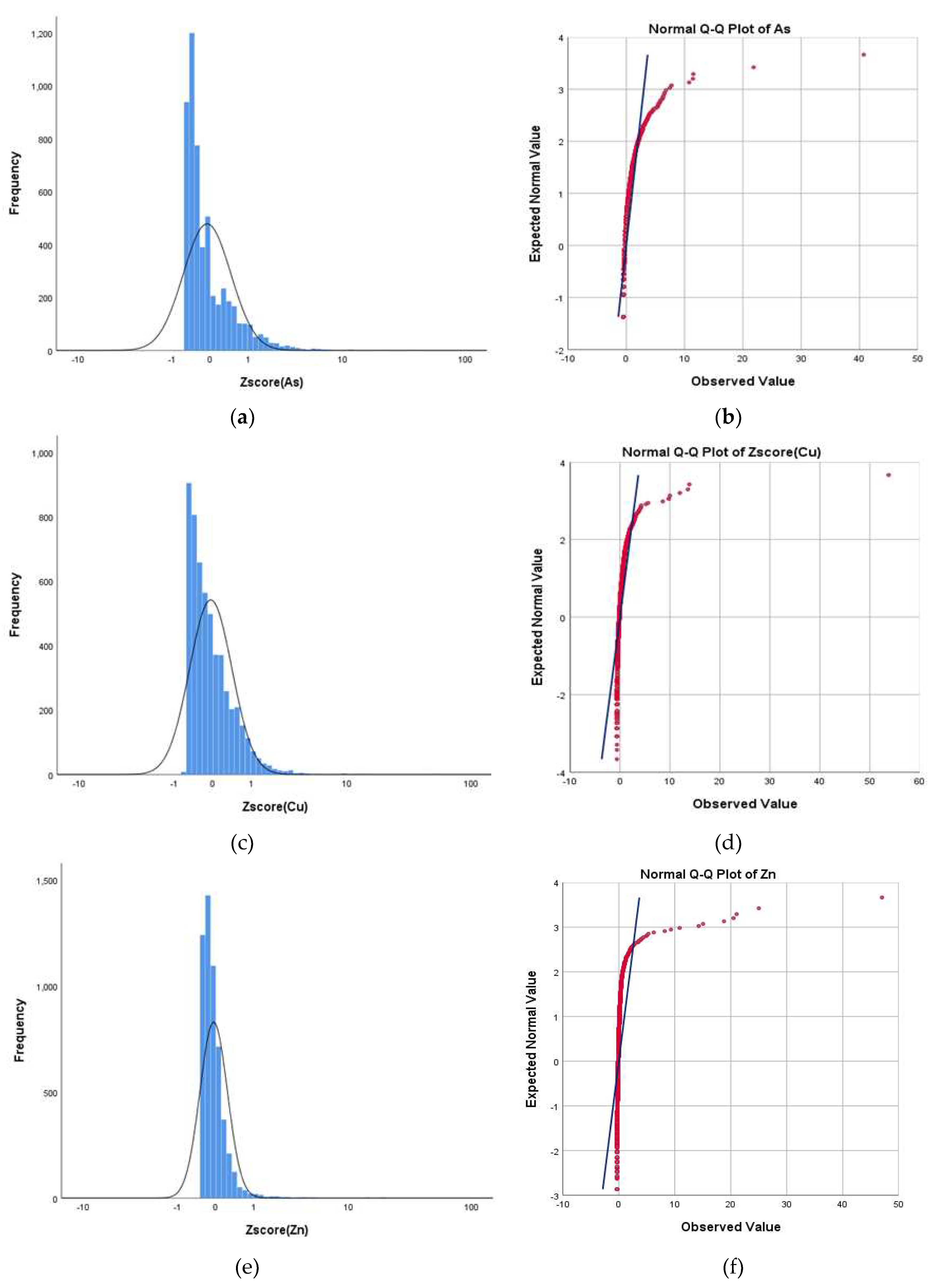
Figure 5.
Raster maps were created from total concentration values of As (a), Cu (c), and Zn (e) in 5,376 samples. The color classes are based on the following percentiles of raw data: 50, 75, 90, and 95 content. Stream sediment values concentrations 95th percentile of As (b), Cu (d), and Zn (f), anomalous represented by red shading overlay with the geologic map, can be divided into the zones of anomalies in NW-SE orientations.
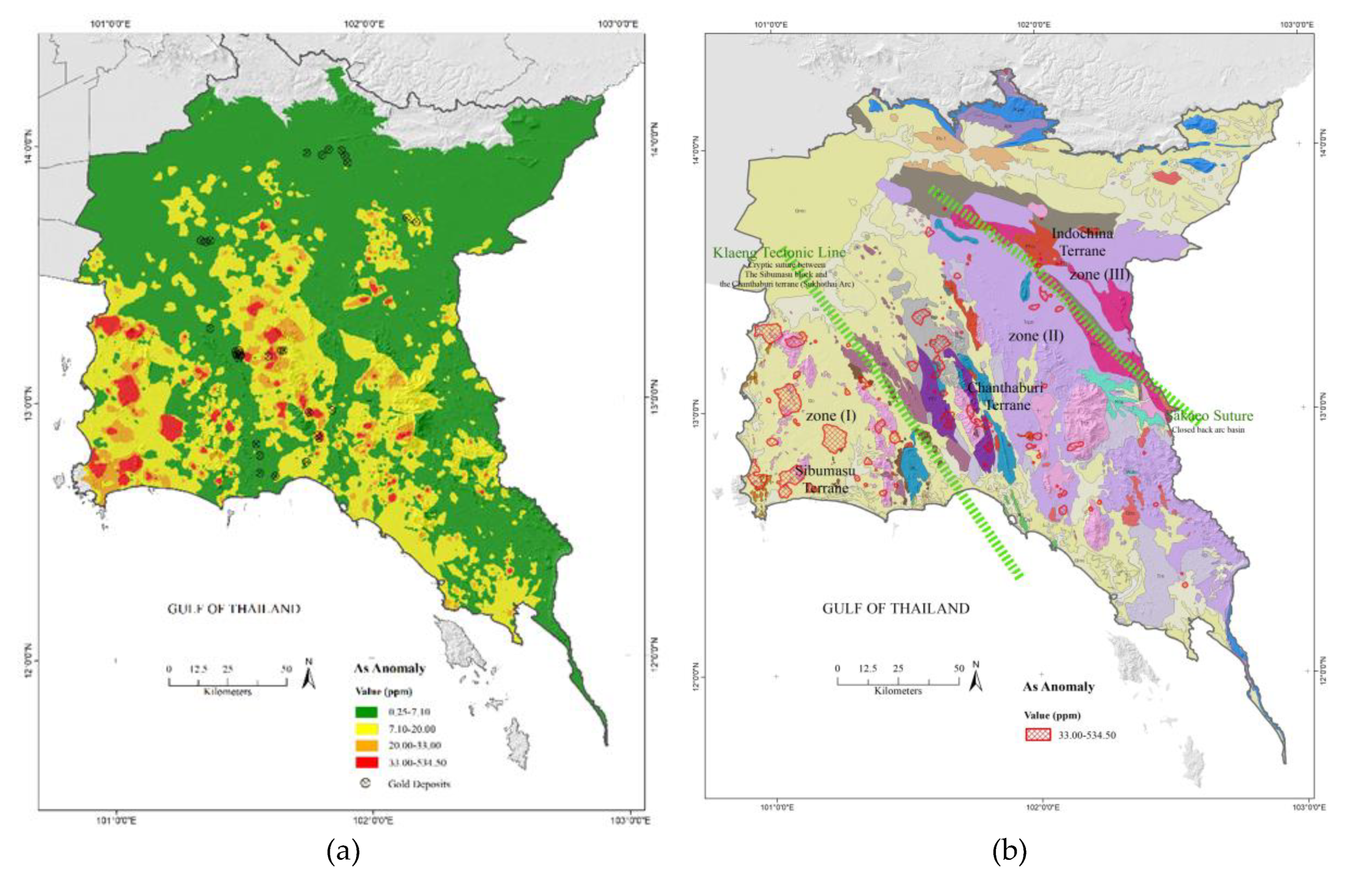
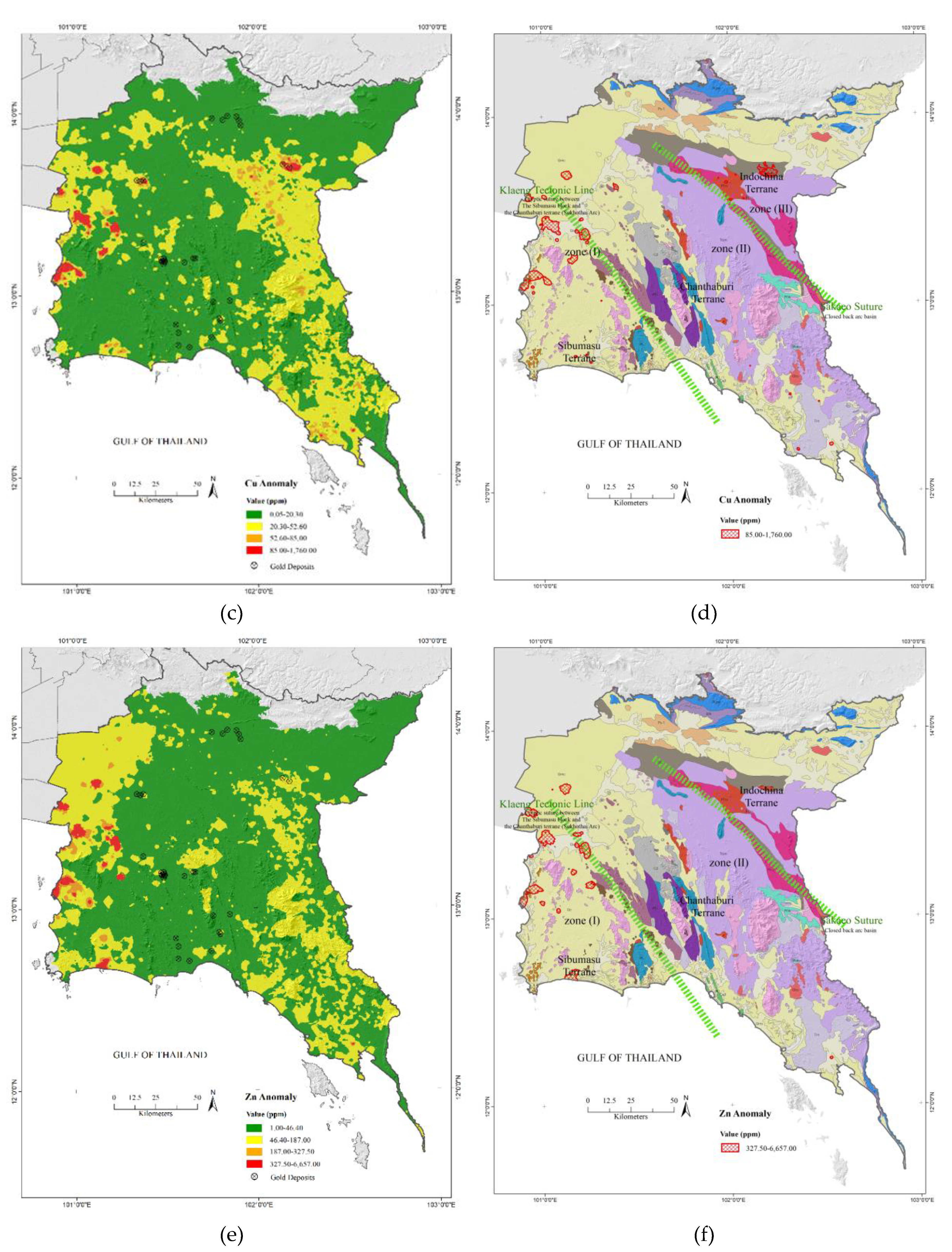
Figure 6.
(a) Log-log plot of spectrum density (S) versus the number of cells greater than or equal to S (log base e) for As. (b) The decomposed map anomaly component and (c) The decomposed map background component of As.
Figure 6.
(a) Log-log plot of spectrum density (S) versus the number of cells greater than or equal to S (log base e) for As. (b) The decomposed map anomaly component and (c) The decomposed map background component of As.

Figure 7.
(a) Log-log plot of spectrum density (S) versus the number of cells greater than or equal to S (log base e) for Cu. (b) The decomposed map anomaly component and (c) The decomposed map background component of Cu.
Figure 7.
(a) Log-log plot of spectrum density (S) versus the number of cells greater than or equal to S (log base e) for Cu. (b) The decomposed map anomaly component and (c) The decomposed map background component of Cu.
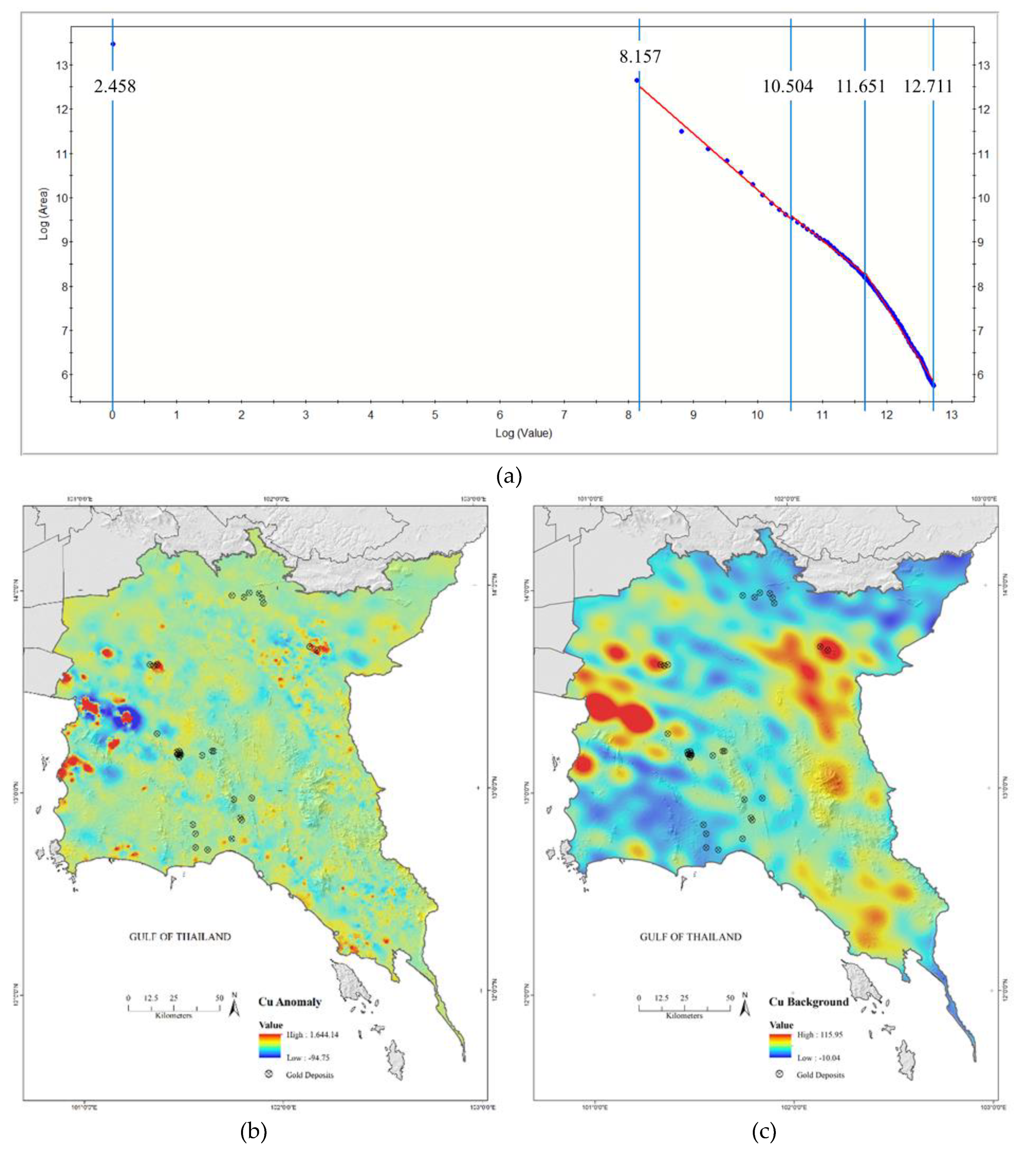
Figure 8.
(a) Log-log plot of spectrum density (S) versus the number of cells greater than or equal to S (log base e) for Zn. (b) The decomposed map anomaly component and (c) The decomposed map background component of Zn.
Figure 8.
(a) Log-log plot of spectrum density (S) versus the number of cells greater than or equal to S (log base e) for Zn. (b) The decomposed map anomaly component and (c) The decomposed map background component of Zn.
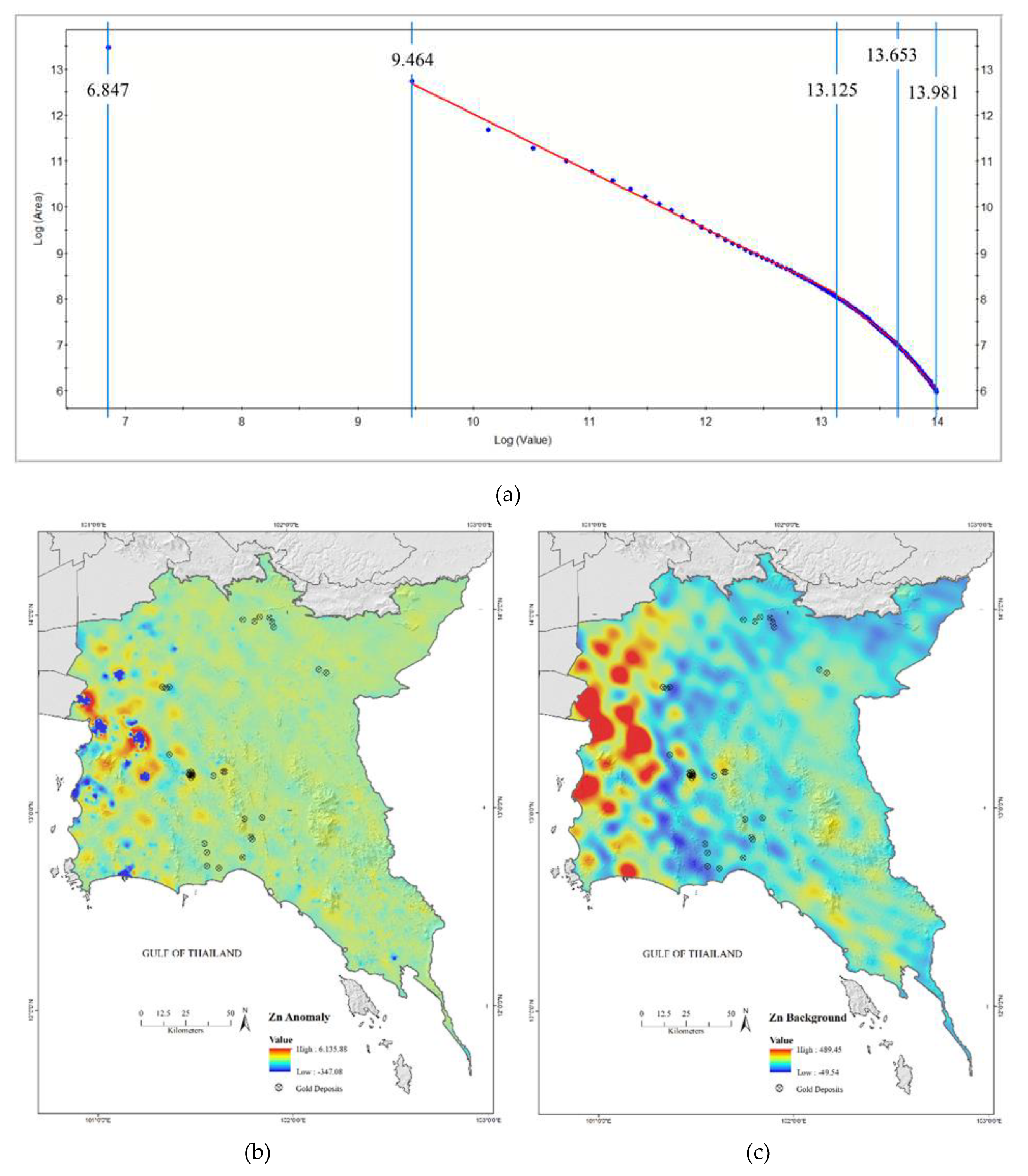

Table 1.
Descriptive statistics for elements of 5,376 stream sediment geochemical data of As, Cu, and Zn used in eastern Thailand.
Table 1.
Descriptive statistics for elements of 5,376 stream sediment geochemical data of As, Cu, and Zn used in eastern Thailand.
| Elements | N | Max | Min | X | SD | CV% | Skewness |
|---|---|---|---|---|---|---|---|
| As | 5,376 | 534.50 | 0.25 | 7.05 | 12.95 | 183.61 | 16.74 |
| Cu | 5,376 | 1,760.00 | 0.05 | 20.26 | 32.36 | 159.75 | 31.25 |
| Zn | 5,376 | 6,657.00 | 1.00 | 46.45 | 140.53 | 302.55 | 6.86 |
Table 2.
Statistical parameters for As, Cu, and Zn Pb (ppm) of the geological unit in eastern Thailand.
Table 2.
Statistical parameters for As, Cu, and Zn Pb (ppm) of the geological unit in eastern Thailand.
|
Geological unit |
Samples (N) | Elements | |||||||||||
| As | Cu | Zn | |||||||||||
| X | SD | Cv | X | SD | Cv | X | SD | Cv | |||||
| Total | 5,376 | 7.05 | 12.95 | 1.84 | 20.26 | 32.36 | 1.60 | 46.45 | 140.53 | 3.03 | |||
| Q | 2,447 | 7.40 | 15.91 | 2.15 | 16.55 | 43.47 | 2.63 | 57.38 | 206.49 | 3.60 | |||
| Ksk | 32 | 2.83 | 4.38 | 1.55 | 31.12 | 12.62 | 0.41 | 47.47 | 11.23 | 0.24 | |||
| Jk | 132 | 5.94 | 10.82 | 1.82 | 6.61 | 6.24 | 0.94 | 13.83 | 12.16 | 0.88 | |||
| Jkl | 5 | 6.00 | 6.27 | 1.04 | 10.14 | 8.07 | 0.80 | 11.60 | 8.73 | 0.75 | |||
| JKpw | 49 | 2.07 | 1.21 | 0.58 | 6.14 | 4.38 | 0.71 | 23.87 | 14.83 | 0.62 | |||
| Jpk | 60 | 5.94 | 10.82 | 1.82 | 6.61 | 6.24 | 0.94 | 13.83 | 12.16 | 0.88 | |||
| Trpn | 1,207 | 6.16 | 8.97 | 1.46 | 22.37 | 12.45 | 0.56 | 38.89 | 18.35 | 0.47 | |||
| Trn | 313 | 6.73 | 6.86 | 1.02 | 26.10 | 15.82 | 0.61 | 40.16 | 21.93 | 0.55 | |||
| PTr | 100 | 19.74 | 17.35 | 0.88 | 17.32 | 7.69 | 0.44 | 32.79 | 17.32 | 0.53 | |||
| Ps-2 | 201 | 19.74 | 17.35 | 0.88 | 17.32 | 7.69 | 0.44 | 32.79 | 17.32 | 0.53 | |||
| Ps-1 | 37 | 3.50 | 6.21 | 1.78 | 15.30 | 12.10 | 0.79 | 27.05 | 18.32 | 0.68 | |||
| Ps | 3 | 5.11 | 2.80 | 0.55 | 22.29 | 18.69 | 0.84 | 22.48 | 16.95 | 0.75 | |||
| C2 | 67 | 22.33 | 14.80 | 0.66 | 15.40 | 6.35 | 0.41 | 39.62 | 31.68 | 0.80 | |||
| DC | 291 | 4.43 | 6.17 | 1.39 | 30.39 | 29.64 | 0.98 | 33.99 | 19.45 | 0.57 | |||
| SD | 26 | 9.03 | 8.43 | 0.93 | 15.71 | 17.57 | 1.12 | 23.96 | 17.47 | 0.73 | |||
| Qbs | 49 | 5.98 | 6.41 | 1.07 | 29.65 | 11.21 | 0.38 | 61.04 | 33.97 | 0.56 | |||
| Trgr | 153 | 9.24 | 12.49 | 1.35 | 15.20 | 12.79 | 0.84 | 36.71 | 27.80 | 0.76 | |||
| PE | 67 | 7.05 | 12.95 | 1.84 | 20.26 | 32.36 | 1.60 | 46.45 | 140.53 | 3.03 | |||
| PTrv/Ptru | 131 | 8.53 | 11.65 | 1.37 | 41.54 | 22.71 | 0.55 | 45.11 | 20.01 | 0.44 | |||
| Pv | 6 | 7.67 | 2.66 | 0.35 | 108.50 | 27.29 | 0.25 | 69.83 | 10.03 | 0.14 | |||
Disclaimer/Publisher’s Note: The statements, opinions and data contained in all publications are solely those of the individual author(s) and contributor(s) and not of MDPI and/or the editor(s). MDPI and/or the editor(s) disclaim responsibility for any injury to people or property resulting from any ideas, methods, instructions or products referred to in the content. |
© 2023 by the authors. Licensee MDPI, Basel, Switzerland. This article is an open access article distributed under the terms and conditions of the Creative Commons Attribution (CC BY) license (http://creativecommons.org/licenses/by/4.0/).
Copyright: This open access article is published under a Creative Commons CC BY 4.0 license, which permit the free download, distribution, and reuse, provided that the author and preprint are cited in any reuse.


