1. Introduction
Logistics is a booming service industry. With the diversity of goods being transported between any two points around the world, one of the quality indicators used by logistics operators is the way goods are manipulated during their transportation. Poor handling may result in damages and/or liability costs to insurance and/or logistics operators.
In engineering terms, this amounts to analyze the trajectories the goods are subject to, i.e., the trajectories resulting from the way they are manipulated during the transportation.
The trajectory reconstruction problem is well known in, for example, the aerospace industry. Using information from IMU attached to the body of the spacecraft, its trajectory can be reconstructed using the velocity and acceleration data and assuming a good model of the spacecraft. Essentially, this amounts to an optimization problem, where the reconstructed trajectory must be such that the data it generates is close to the observed data. The literature on the problem is vast, see for instance [
1] on using multiple models and Unscented Kalman Filtering (UKF) [
2] on using Extended Kalman Filtering (EKF) techniques and inertial measurement data [
3] on using image data, [
4] on using Gaussian regression techniques and GPS data.
The extension to the logistics problem introduces additional constraints, namely, sensing must be really cheap (i.e., the quality of the accelerometers and rate-gyros is nowhere close to that used in the aerospace industry), and the rigidity of the goods is only loosely verified. For example, goods such as food or domestic appliances are often transported in cardboard boxes and hence, rigidity is valid under the assumption that handling forces are relatively small or highly localized to avoid damages. Moreover, the placement of the sensors will, in general, be made by unskilled/carefree operators which may lead to devices malfunctioning and hence redundancy, as with using multiple (similar) devices, is likely to increase the amount of usable information for trajectory reconstruction.
The vision of the paper to implement this redundancy is that of a network of low cost IMUs that can be glued-and-forgotten in typical packages (made out of cardboard, wood, plastic, metal, etc). These IMUs can be either be placed (i) forming a regular, pre-defined, pattern, with the packages specifying precise areas where to “glue” the devices, or (ii) distributed through the package arbitrarily. Placing the devices must not require any special expertise. The first scenario is possible in packages of standardized dimensions and limits the need for calibration procedures. In the second scenario some calibration procedure may be necessary prior the start of the transportation. For the sake of simplicity, this paper assumes that the whole IMUs in the network are placed at the same point. This does not imply any lack of generality; in a real scenario, with all IMUs placed in different locations, the reconstructed trajectories would differ among them by constant homogeneous transformations.
Having multiple IMUs gathering data and combining it to reconstruct the trajectory may, in principle, improve the robustness of the solution, as (i) the amount of data increases and it may contain richer information, and (ii) redundancy helps dealing with sensor fails. Combining
a posteriori the solutions found, from the data collected from each IMU independently of each others, e.g., using covariance intersection or some other averaging method, is a possibility and does not require exchange of information among nodes. The alternative, followed in this paper, is to have a network of nodes, each including (i) sensory information from a local IMU and (ii) communication with other distributed nodes (of similar architecture) to the exchange of information
1. The novel approach presented here follows from a multi-target tracking problem first presented in [
5], re-interpreted as a consensus generation in a network of IMUs. The motivation to use this formulation comes from the proven optimality of the framework in [
5] in the context of the multi-tracking problem.
The paper is organized as follows.
Section 2 illustrates a single, simulated, IMU, establishing a baseline performance for comparison with the consensus approach.
Section 3 presents a quick view of the work in [
5], which serves as a basis for this work, focusing on the consensus features and clarifying the re-interpretation of the key terms. Moreover, the feasibility problem, i.e., the existence of a strategy for the exchange of information such that all nodes in the network can provide estimates of the reconstruction, is discussed using the Linear Matrix Inequalities (LMI) framework.
Section 4 illustrates the evolution of performance indicators of simulated nodes recovered from the network framework when the communications among them are inhibited.
Section 5 presents simulation results with simple networks with 2 and 3 nodes.
Section 6 discusses the improvement of the network consensus over reconstruction by independent nodes.
Section 7 presents results on the fusion of the trajectories reconstructed by each node using Covariance Intersection. Finally,
Section 8 concludes the paper with a discussion on the feasibility of the approach and points to future research.
2. Baseline IMU
Given an arbitrary trajectory that serves as the ground truth, the corresponding linear and angular accelerations can be easily obtained if the inertia properties of the body (assumed rigid) moving over the trajectory are known. Thus, to accurately simulate the sensors to be glued to the logistics packages knowledge of the inertia properties of the package is required beforehand.
In practical terms, full knowledge about package inertia will seldom be available (though mass and the physical dimensions can be easily known
a priori as they are the parameters that directly influence the transportation cost). Therefore, while the observations reflect the real properties of the packages, the reconstruction of the trajectories has only a limited amount of that knowledge available. However, it should be emphasized that estimation of mass/inertia properties can also be done using IMU data. This is a well known problem in aerospace industry, see for instance [
6] on using recursive least squares, [
7] on using continuous systems identification techniques to identify the dynamics of the Hubble telescope, [
8] on using the LMI framework and formulating a least squares problem, and [
9,
10] on using the least squares formulation combined with S-estimators for the identification of spacecraft parameters.
The basic approach to estimate the trajectory from velocities and accelerations is to use simple integrator models. Given a trajectory expressed in terms of the position and orientation coordinates,
, assume that the corresponding signals from accelerometers and rate-gyros can be obtained from
where
are the corresponding sensor outputs, i.e., linear accelerations and angular velocities, respectively. Also,
stand for
and
, respectively. The purpose of these expressions is to yield a simulation tool and, without lack of generality, they implicitly assume a unit mass body. To improve realism, noise can be added to the outputs of these sensors.
2.1. Dead Reckoning Experiments
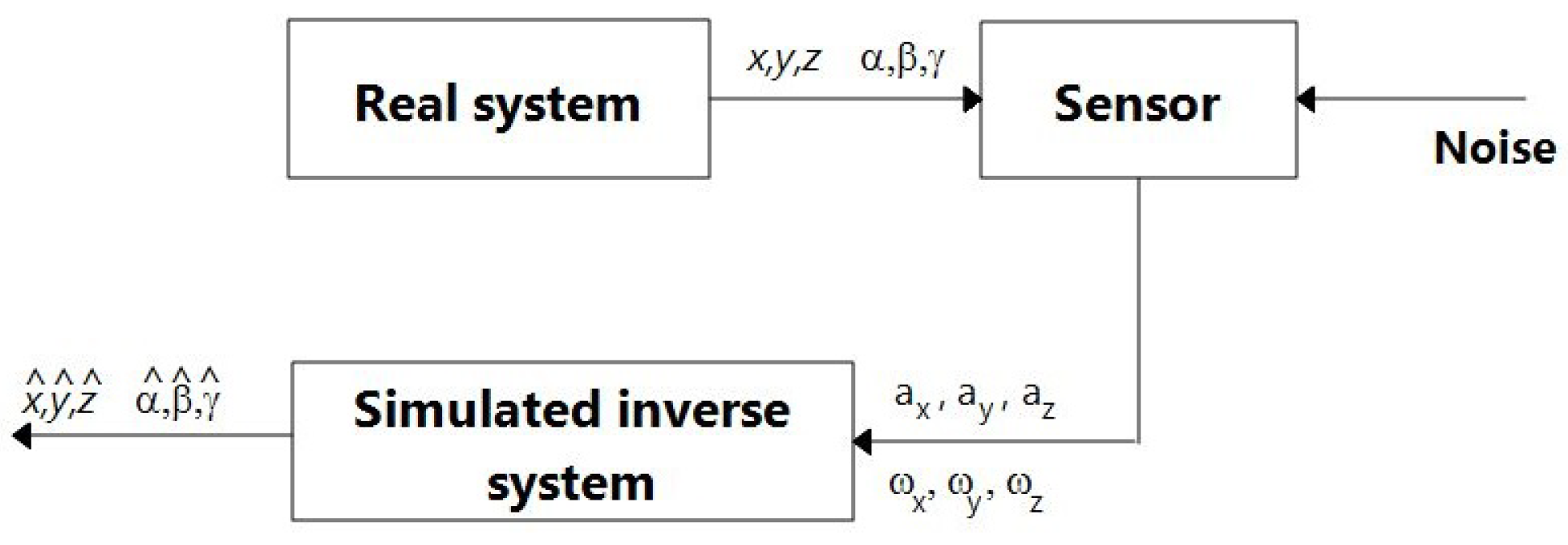
The purpose of these experiments is (i) to show the effects of noise when no compensation strategy is used, and (ii) to serve as baseline to compare with the network experiments. Using sensor data as obtained from (
1), corresponding to some reference trajectory, and a dead reckoning model, the goal is to reconstruct the reference trajectory.
Figure 1.
Dead reckoning trajectory reconstruction. Good estimates can be obtained if the model of the system is accurate and the effect of noise minimized.
Figure 1.
Dead reckoning trajectory reconstruction. Good estimates can be obtained if the model of the system is accurate and the effect of noise minimized.
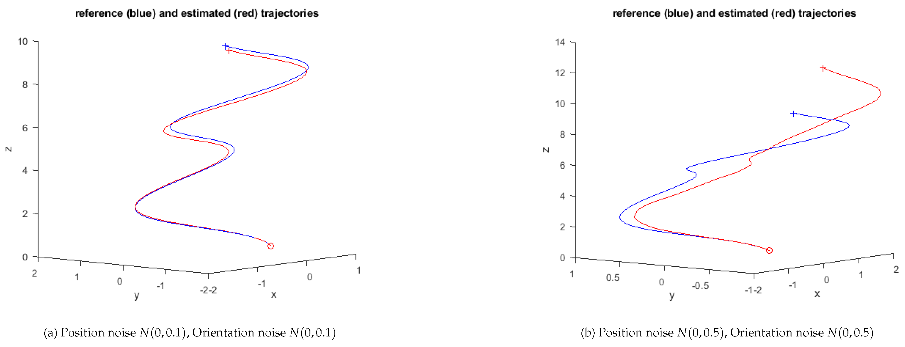
Sensor uncertainties make the reconstructed trajectory deviate from the real one.
Figure 2 illustrates the effects of such situations, for two levels of position noise.
From the perspective of a logistics application this simple approach may still be a valid option if disturbances are limited and only specific events are relevant to measure the quality of the handling, e.g., if the existence of strong nonsmooth/disturbances areas is required. In such cases, even if the reconstructed trajectory in the cartesian 3D space differs significantly from the real one, the presence of areas of strong disturbances can still be recognized and it is the relevant event in what concerns assessing the quality of the handling.
The existence of drifts in the observed variables is another important disturbance factor. Poor assembly of a sensor, electronics issues, are common causes of drifts. In the accelerometer, drift means that the dynamics of the acceleration is constantly integrating some value that is not being observed by the accelerometer. In the case of the rate-gyro, this means that the dynamics of the rotational velocity is constantly integrating some value that is not being directly observed by the gyro.
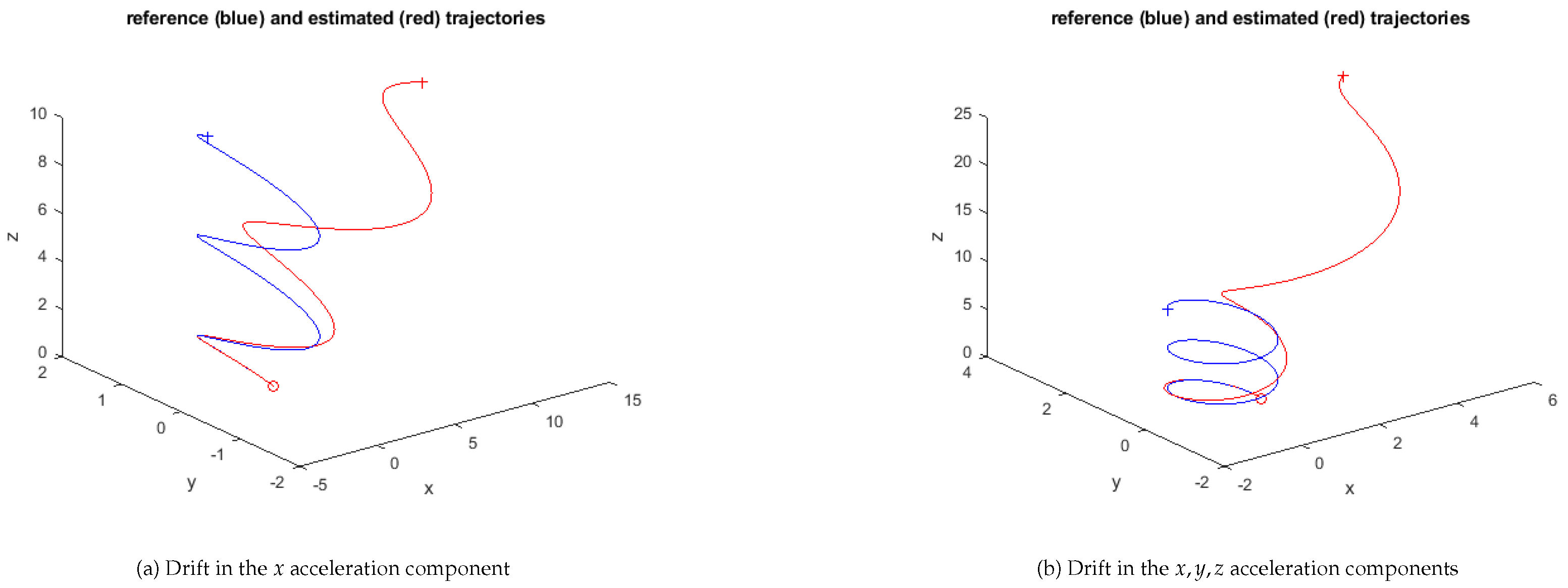
Figure 3 illustrates two experiments of the dead reckoning approach under constant drift conditions.
The disturbances considered affect only the linear acceleration. In the first sample they are given by
where
stands for the usual function returning a random value with a
distribution. In the second sample all the coordinates are similarly affected by a term,
.
Figure 3.
Dead reckoning experiment, spiral x-y-z trajectory, under drift conditions (Wiener process)
Figure 3.
Dead reckoning experiment, spiral x-y-z trajectory, under drift conditions (Wiener process)
This is an example where the estimated trajectory is too different from the original one. However, depending on specific requirements of the logistics application, drift disturbances may not be an issue, e.g., as mentioned above if the purpose is the detection of harsh handling. Clearly, drifts are highly relevant if accurate trajectory reconstruction is required, which is the focus of the remainder of the paper.
3. Background
This paper adopts the formulation from [
5], developed in the context of a multi-target tracking problem with targets and measurements assumed to have a one-to-one relation. The notation follows the usual form of the continuous-discrete (CD) extended Kalman framework (see for instance [
11] for a critical comment and implementation issues of this form), with the prediction stage for the
i-th IMU node given by (see also [
12] for a face-off between five different formulations),
where
F is the Jacobian of
f, and the modified update stage,
where
H is the Jacobian of
h, and with the networking and consensus being expressed through the measurement uncertainties,
using
measurements
(received by the
i-th IMU from the
j-th IMU, i.e., the
i-th IMU is connected to
other IMUs ) and with the weighted innovations,
where
is the weight expressing the relevance of measurement from node
j to the estimate of the measurement by node
i,
is the weight expressing the relevance of poor measurements (
amounts to reducing the norm of
, forcing the covariance to decrease even if poor measurements are being fed into the system), and
, the estimate of the measurement of the
i-th node at instant
k, that is,
, and
, the actual measurement of node
j at instant
k reaching the
i-th IMU.
The topology of the network is assumed fixed. In [
5], the
parameters were interpreted in terms of a marginal probability of association between node
j and target
i. The
is used to quantify misdetection of a target (1/0 for misdetected/detected). However, for the purpose of this paper, this interpretation is not useful as the association between nodes and measurements can be known a priori. Instead, these parameters can be seen as (i) the communications protocol (as in consensus problems), and (ii) scaling weights for the measurements. Also, as in the original problem, the number of measurements,
, can vary along time (or measurement scans)
k.
The formulation from [
5] is, essentially, an EKF with a modified update of the covariance matrix (through the
factor that scales the innovation residual covariance, (
3), and a weighted combination of the innovations from the whole network weighted by the
. Also, (6), dumps the term explicit in the noise
, and the symmetric term
affecting
in the CD formulation of the EKF.
This innovates relative to the CD-EFK procedure in that the covariance of each unit now has feedback from the innovations produced by the network. Moreover, the tuning “knob” in the CD-EKF formulation is now replaced with the and parameters. These can also be seen as the mediators/protocol/sacling factors between the nodes.
For the sake of readability, the expression for the covariance update in the CD-EKF formulation and a re-writing of (6) to highlight the differences to the CD-EKF covariance update equation, is presented below.
The renewed one, where
and
are
matrices is,
The first two terms on the righthand side of (
10) are also present in (
9). The third and fourth terms, account for the network exchanges, is the additional `tuning knob”. The fifth term dampens the second term and provides additional control.
The convergence of (
10) can be achieved by careful selection of
and
, namely ensuring that
is a contracting sequence converging to some fixed point (see [
13]). This means
or, alternatively,
or, in a more compact form to highlight the terms involved in the consensus, with
,
, and
,
At each time step a new solution must be produced so that the convergence of the covariance matrix can be controlled. This means that (i) the consensus will be adjusting over time, as the will (in general) be changing, and (ii) tradeoff values for (that can be constant over time) has to be selected. However, one must ensure that the can be made unique during the whole duration of the trajectory, despite the changes in the .
Making,
the solution of
can be obtained using the LMI form (see for instance [
14], pp. 7-8, on computing maximum singular values) as,
The complete solution for the convergence of (
10) requires an additional LMI that imposes the positive definiteness of
given that
is assumed positive definite,
or, more compactly, with
,
Therefore, if (
11) and (
12), with the
variables, are both feasible at each time step,
k, for some choice of
, then there is a consensus solution to the network, from the point of view of the
i-th node, which ensures the convergence of
.
A solution for the full network requires the feasibility of the above LMI problems for all the nodes.
LMI feasibility can be tested by multiple algorithms, from general ones, [
15,
16] on ellipsoid algorithms, to specific ones, [
17] for large and sparse LMIs or [
18] on stochastic algorithms. Several software packages to solve LMIs are available, i.e., the Scilab based LMITOOL,[
19], the Matlab based YALMIP, [
20], and the Matlab LMI toolbox.
These LMI problems are non-convex (the presence of the affine term in (
12) is enough to make it non-convex) and hence finding optimal parameters using standard LMI solvers is, in general, an issue. Relaxation techniques are commonly used to solve non-convex problems. and obtain either good solutions or pseudo-solutions from which approximations to the good ones can be derived (see, for instance, [
21,
22,
23]). The approach proposed here uses a basic form of relaxation, consisting in scaling some terms until a solution can be found.
4. Simulation Experiments
Making
and
, then
for
, recovering a set of isolated nodes and
and the convergence condition becomes,
Given that all the matrices in (
13) are norm-bounded then the 2nd condition can always be verified for large enough
and small enough
.
The noise covariance
bounds the definiteness of (
13) (in the best possible scenario
; in general this is not a free parameter as it must be chosen in connection with the sensors, though it can also act as a tuning knob to some extent). The matrix
is, by construction, always positive definite and hence the quadratic term
is also positive definite. By introducing a scale factor
in
, the LMI (
14) dominates that in (
13), i.e., the set of solutions
of (
14) contains those of (
13) (see [
24] for detailed analysis and results related to LMI dominance).
Given the scaled expression
as
the solution
converges to that of the unscaled expression. Also, as
,
, which is by construction positive definite.
Given the low complexity of the scaled expression, its feasibility relative to the
parameter can be obtained from the eigenvalues/eigenvectors of the matrix
Positiveness of all eigenvalues means
. As the
varies, the eigenvalues of the relaxed matrix are linearly related to those of
.
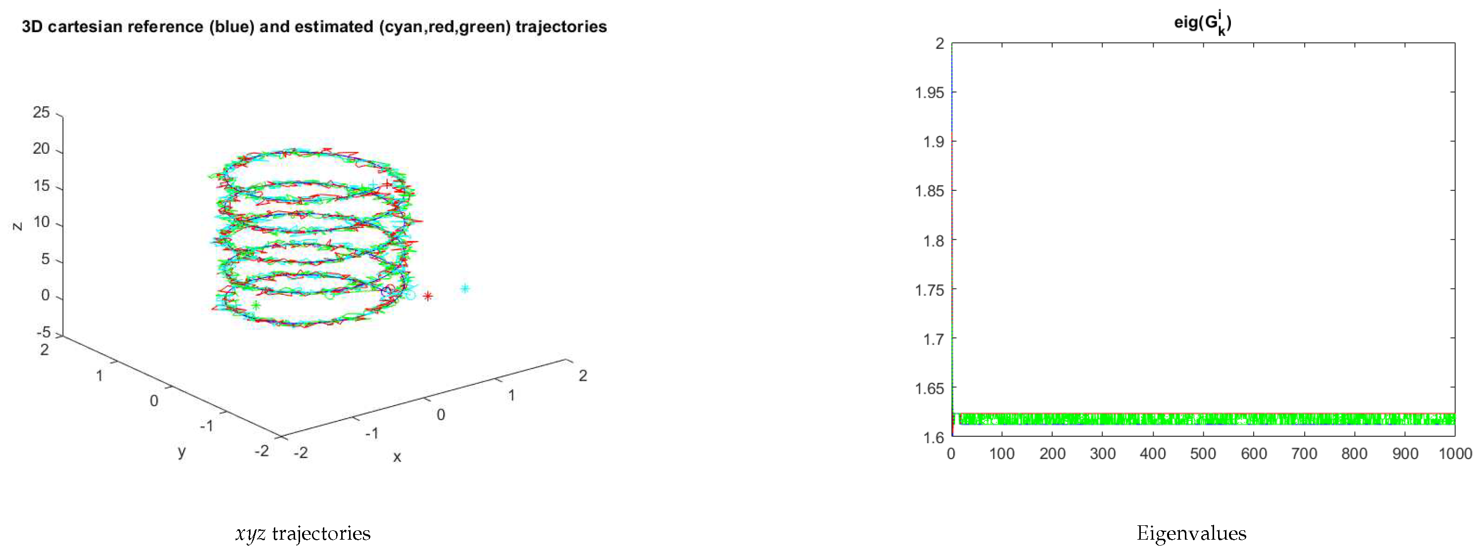
Figure 4 shows an example of the evolution of the eigenvalues using
As expected, the quality of this solution, using the EKF, is clearly superior to that in the example on dead reckoning.
Whenever the nodes are not independent and the network must reach a consensus the feasibility must be checked directly using (
11) and (
12).
5. Network Consensus Experiments
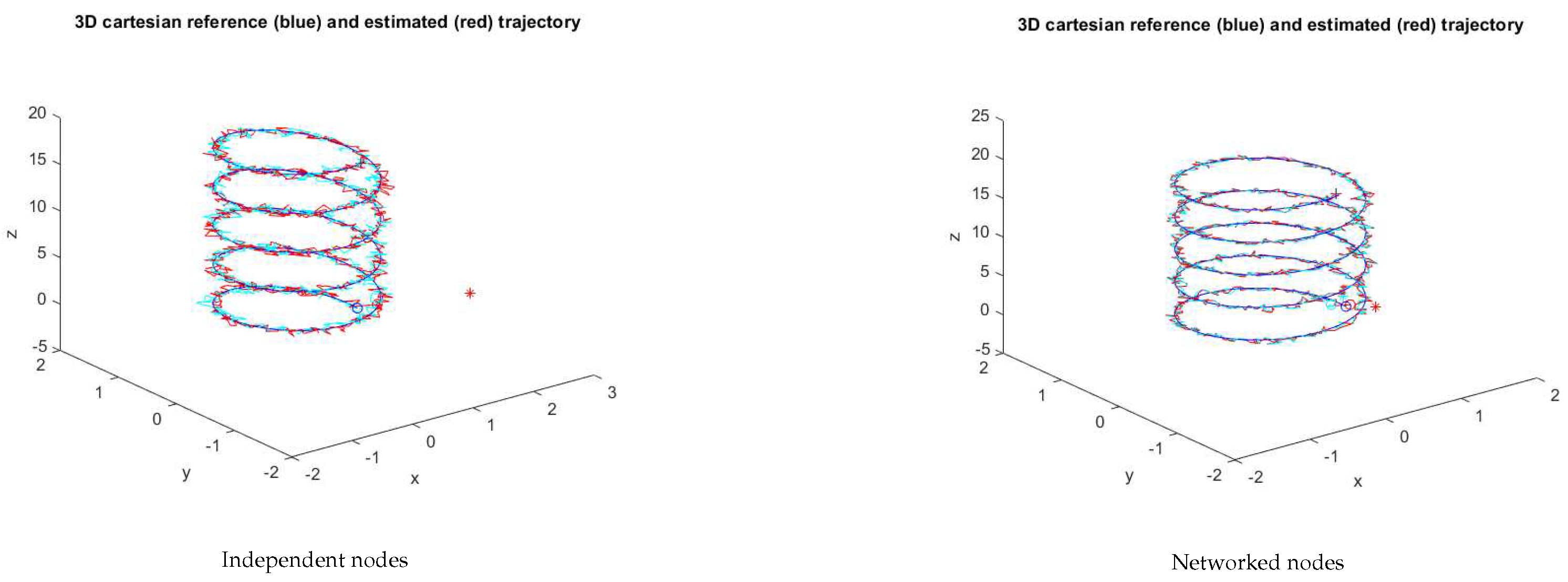
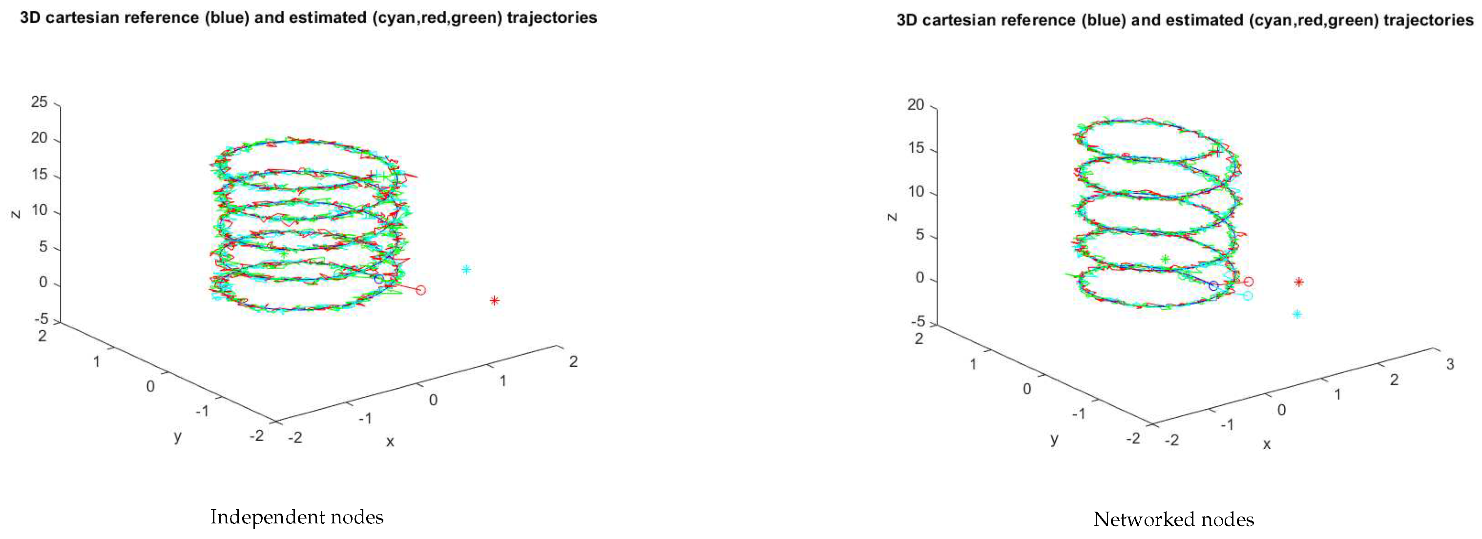
Figure 5 shows the 3D space trajectories for the 2 nodes operating independently and as a network. All IMUs assumed time-synchronized, i.e., the simulation loop time is the same for all of them. For the independent nodes test,
,
. For the networked nodes test,
,
. Any of the IMU trajectories can be used for reconstruction purposes.
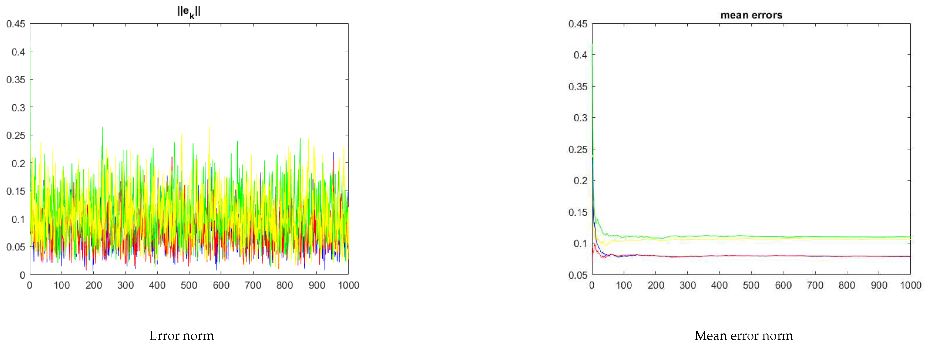
Figure 6 shows the evolution of the 2-norm of the
trajectory and of the respective mean. Clearly, the mean error when the nodes operate cooperatively is lower than when operating independently.
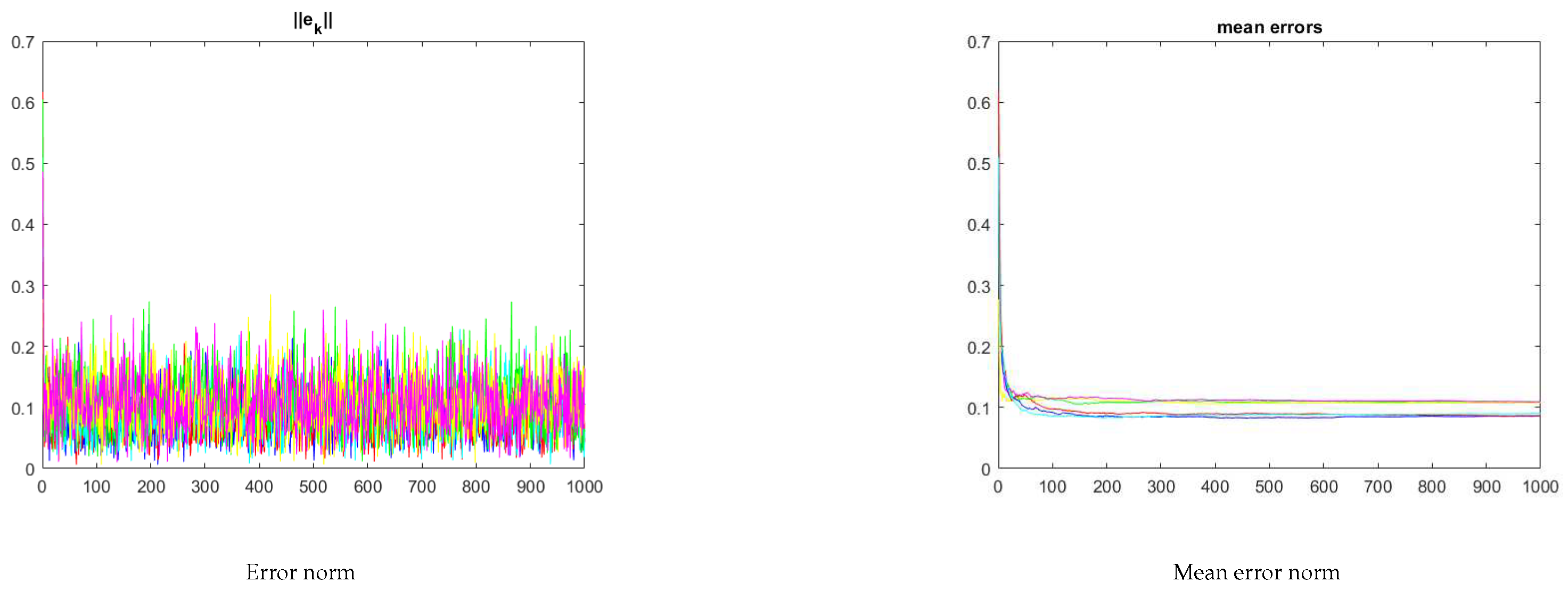
Figure 7 and
Figure 8 show a similar experiment with 3 nodes. For the independent nodes test,
,
. For the networked nodes test,
,
.
For the three-node network the mean error of the trajectory of the networked nodes is also lower than the error for the independent nodes.
Figure 8.
Three node network error evolution for the sample in
Figure 7 (the red/blue/cyan curves refer to the networked nodes; the yellow/green/magenta curves in the righthand plot refer to the independent nodes under no-consensus).
Figure 8.
Three node network error evolution for the sample in
Figure 7 (the red/blue/cyan curves refer to the networked nodes; the yellow/green/magenta curves in the righthand plot refer to the independent nodes under no-consensus).
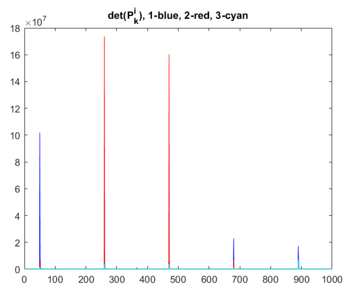
The evolution of the feasibility conditions, i.e., (
11) and (
12), is shown in
Figure 9.
Figure 9.
Feasibility evolution () for the 3 node experiment.
Figure 9.
Feasibility evolution () for the 3 node experiment.
From a practical perspective, if during a reconstruction the LMI problem returns unfeasible then simply use one of the independent units as solution.
6. Networking for Improvement over Independent Nodes
As seen before, the feasibility of a network can be tied to a LMI. Also, the experiments in the previous section empirically show that networks have and advantage over independent nodes. The purpose of this section is to demonstrate this advantage, i.e., the difference between the tracking errors obtained in the networked and independent versions,
where
r is the reference trajectory,
is the trajectory reconstructed by a network, and
is a trajectory reconstructed by one node operating independently, verifies the averaging relation
For a discrete, time varying, linear system, Lemma 3.1 in [
25] states that
is bounded above and below, i.e.,
.
is a linear operator on
and hence it is also bounded above and below.
is also bounded as depends on the bounded
and on
which is also upper and lower bounded. Therefore,
is bounded and, also, the whole rightmost term in (
15) can be written as
for some
and
a suitable identity matrix.
Applying a 2-norm on both sides of an inequality preserves the inequality, as this norm is monotone [
26], and the righthand term can thus be assumed to be a bounded function,
The leftmost term in (
15) is a function of the
parameters. Without loosing generality, one can represent this term as,
with
adequate functions. Therefore, (
15) can be written as,
Under the LMI feasibility conditions,
and
are bounded and hence by selecting small enough
constants the rightand side of (
17) approaches
The feasibility of the LMI problem ensures the asymptotic convergence of and hence it is clear that, if the networked version converges to the reference trajectory r, the are negative.
The consensus approach can also be beneficial in case of structured unmodelled disturbances, as in the case of unmodelled drift in the sensors. From
Figure 10, the consensus approach retains the good property of low mean error when compared with the nonconsensus approach.
Figure 11 illustrates the performance in the case of a piecewise linear (2 trunks) reference trajectory. As before the mean error property is verified.
7. Network Fusion Using Covariance Intersection
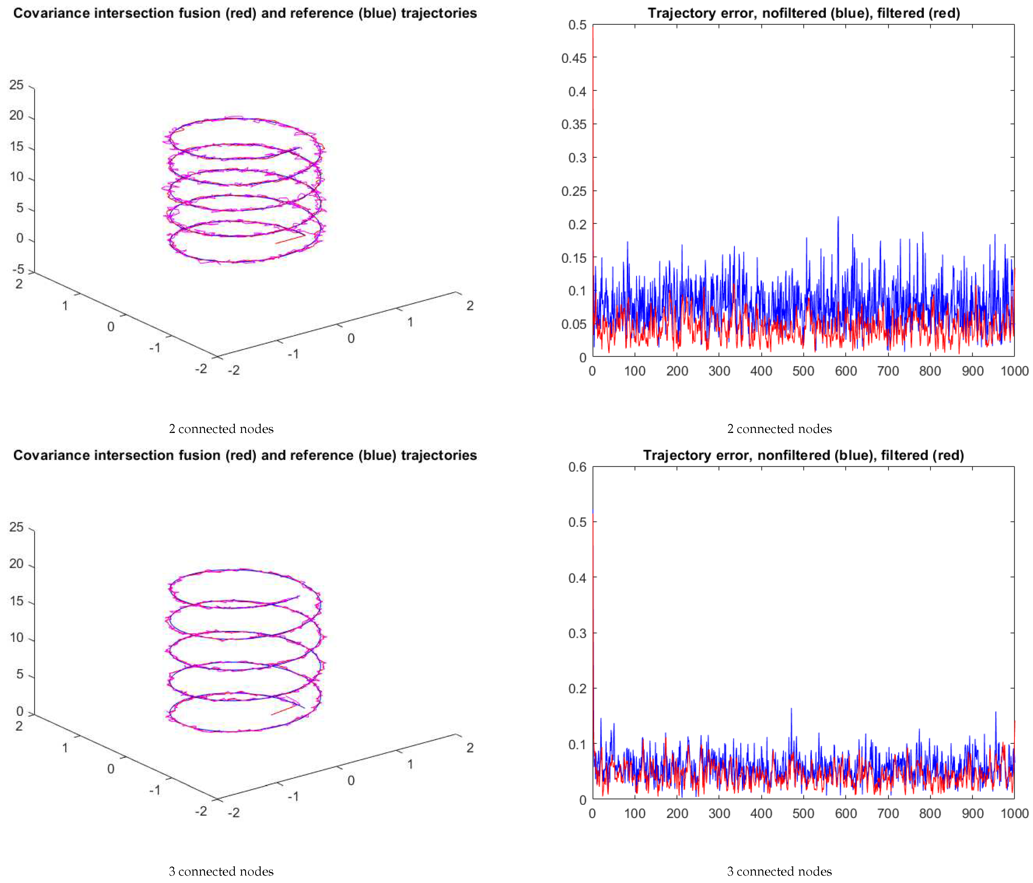
The framework above leads to each IMU producing its own estimate, each of which better than the independent estimates. A single estimate can be obtained by applying the covariance intersection procedure [
27].
Figure 12 shows the resulting trajectories for the spiral reference trajectory in the case of 2 and 3 nodes, respectively. In both cases a median filter with a 20 samples sliding window is used to smooth the output of the fusion stage. In this example, the fusion of the 3 nodes yields a smaller tracking error trend when filtered.
8. Conclusions
The paper presented a formulation for networks of IMUs, extending a representation of the multi-target problem discussed in the literature. Feasibility conditions are discussed based on the feasibility of LMIs modeling the network. Moreover, the network with consensus version (with the nodes exchanging information among them) is shown to have an edge over the non-consensus network (i.e., with independent nodes).
Future work may involves multiples research directions. A natural evolution is the testing of alternative formulations for the EKF, e.g., the discrete formulation (which, being computationally simpler may lead to numerical problems). Also, more complex protocols need to be tested and stronger connections with the consensus theory investigated. Essentially this amounts to replace the by adequate functions, able to shape the interchange of information among nodes.
As referred in the introduction, the rigidity assumption in the relative positioning of the IMUs is likely not to hold permanently. Rigidity criteria that can be used to determine performance bounds of the consensus approach will be a key research topic in this framework.
In the paper it is implicitly assumed that data is acquired, synchronously, and immediately processed for reconstruction. However, it should be emphasized that data acquisition and reconstruction can occur sequentially in time, i.e., data is acquired during the traveling, after which it can be downloaded and fed into the reconstruction stage. Moreover, this decoupled strategy allows the testing of different parameters for reconstruction. Also, synchronicity in data acquisition is likely not to hold for the whole duration of a mission (e.g., due to mishandling of packages which can damage the devices, intrinsic failures, electronics interferences, etc) and hence strategies to minimize the effect of missing data are to be investigated.
The advantage of combining covariance intersection and consensus was illustrated in the simple example above, when data is synchronized. Additional testing including asynchronous data scenarios, e.g., as in [
28,
29], is scheduled for future work.
Funding
This work was partially supported by project LARSyS-FCT Project UIDB/50009/2020.
Data Availability Statement
All software available on reasonable request to the author.
Conflicts of Interest
The author declares no conflict of interest.
Abbreviations
The following abbreviations are used in this manuscript:
| IMU |
Inertial Measurement Unit |
| LMI |
Linear Matrix Inequality |
| EKF |
Extended Kalman Filter |
| CD-EKF |
Continuous-Discrete Extended Kalman Filter |
References
- Huang, P.; Zhang, C.; Li, H.; Shi, F. Research on Real-Time Reentry Trajectory Reconstruction Base on Multiple Model. In Proceedings of the Procs of the 40th Chinese Control Conference, 2021. July 26-28, Shanghai, China.
- Karlgaard, C.; Tartabini, P.; Blanchard, R.; Kirsch, M.; Toniolo, M. Hyper-X Post-Flight-Trajectory reconstruction. Journal of Spacecraft and Rockets 2006, 43. [Google Scholar] [CrossRef]
- Liu, J.; Ren, X.; Yan, W.; Li, C.; Zhang, H.; Jia, Y.; Zeng, X.; Chen, W.; Gao, X.; Liu, D.; Tan, X.; Zhang, X.; Ni, T.; Zhang, H.; Zuo, W.; Su, Y.; Wen, W. Descent trajectory reconstruction and landing site positioning of Chang’E-4 on the lunar farside. Nature Communications 2019, 10. [Google Scholar] [CrossRef] [PubMed]
- Takahashi, Y.; Saito, M.; Oshima, N.; Yamada, K. Trajectory reconstruction for nanosatellite in very low Earth orbit using machine learning. Acta Astronautica 2022, 194, 301–308. [Google Scholar] [CrossRef]
- He, S.; Shin, H.; Tsourdos, A. Distributed Joint Probabilistic Data Association Filter with Hybrid Fusion Strategy. IEEE Transactions on Instrumentation and Measurement 2019. [Google Scholar] [CrossRef]
- Wilson, E.; Lages, C.; Mah, R. On-line, gyro-based, mass-property identification for thruster-controlled spacecraft using recursive least squares. In Proceedings of the Proc. 2002 45th Midwest Symposium on Circuits and Systems (MWSCAS-2002), 2002. 4-7 august, Tulsa, Ok, USA.
- Anthony, T.; Andersen, G. On-Orbit Modal Identification of the Hubble Space Telescope. In Proceedings of the Proc. American Control Conference, 1995. June, Seattle, Washington.
- Keim, J.; Açıkmeşe, B.; Shields, J. Spacecraft inertia estimation via constrained least squares. In Proceedings of the Proc. IEEE Aerospace Conference, 2006. 4-11 March, Big Sky, MT, USA. [CrossRef]
- Milhano, T.; Sequeira, J.; Di Sotto, E. Using S-estimators in Parameter Identification. In Proceedings of the Proc. 16th Internationl Conference on Information Fusion (Fusion 2013), 2013. 9-12 July, Istanbul, Turkey.
- Milhano, T.; Sequeira, J.; Di Sotto, E. Spacecraft Parameter Identification Using S-Estimators. In Proceedings of the Proc. 9th International Conference on Guidance, Navigation & Control Systems (GNC 2014), 2014. 2-6 June, Porto, Portugal.
- Guihal, J.; Auger, F.; Bernard, N.; Schaeffer, E. Efficient Implementation of Continuous-Discrete Extended Kalman Filters for State and Parameter Estimation of Nonlinear Dynamic Systems. IEEE Transactions on Industrial Informatics 2022, 18, 3077–3085. [Google Scholar] [CrossRef]
- Salau, N.; Secchi, A.; Trierwieler, J. Five Formulations of Extended Kalman Filter: Which is the best for D-RTO? 17th European Symposium on Computer Aided Process Engineering – ESCAPE17; Plesu, V.; Agachi, P., Eds. Elsevier B.V., 2007.
- Lohmiller, W.; Slotine, J. On Contraction Analysis for Nonlinear Systems - Analyzing stability differentially leads to a new perspective on nonlinear dynamic systems, 1997.
- Boyd, S.; El Ghaoui, L.; Feron, E.; Balakrishnan, V. Linear Matrix Inequalities in System and Control Theory; SIAM - Society for Industrial and Applied Mathematics, Philadelphia, 1994.
- Vandenberghey, L.; Balakrishnan, V. Algorithms and Software for LMI Problems in Control. In Proceedings of the Procs. IEEE International Symposium on Computer-Aided Control System Design, 1996. Dearborn, Michigan.
- Im, K.H.; Baang, D. Optimized ellipsoid algorithm for LMI feasibility problems. International Journal of Control, Automation and Systems 2014, 12, 915–917. [Google Scholar]
- Zhang, R.; Lavaei, J. Efficient Algorithm for Large-and-Sparse LMI Feasibility Problems. 2018 IEEE Conference on Decision and Control (CDC), 2018. Miami, FL, USA, 17-19 December. [CrossRef]
- Calafiore, G.; Polyak, B. Stochastic Algorithms for Exact and Approximate Feasibility of Robust LMIs. IEEE Transactions on Automatic Control 2001, 46, 1755–1759. [Google Scholar]
- Nikoukhah, R.; Delebecque, F.; El Ghaoui, L. LMITOOL: a Package for LMI Optimization in Scilab User’s Guide. Technical report, INRIA, RT-0170, ffinria-00070000, 1995.
- Löfberg, J. YALMIP : A Toolbox for Modeling and Optimization in MATLAB. Procs. of the CACSD Conference;, 2004.
- Eltved, A. Convex Relaxation Techniques for Nonlinear Optimization. PhD thesis, Technical University of Denmark, 2021.
- Bi, Y. Analysis of Convex Relaxations for Nonconvex Optimization. PhD thesis, Cornell University, 2020.
- Keller, A. Convex underestimating relaxation techniques for nonconvex polynomial programming problems: computational overview. Journal of the Mechanical Behavior of Materials 2015, 24, 129–143. [Google Scholar] [CrossRef]
- Helton, J.; Klep, I.; McCullough, S. Relaxing LMI Domination Matricially. In Proceedings of the Procs. 49th IEEE Conference on Decision and Control (CDC), 2010. 15-17 December, Atlanta, GA, USA. [CrossRef]
- Elizabeth, S.; Jothilakshmi, R. Convergence Analysis of Extended Kalman Filter in a Noisy Environment Through Difference Equations. International Journal of Pure and Applied Mathematics 2014, 91, 33–41. [Google Scholar] [CrossRef]
- Johnson, C.; Nylen, P. Monotonicity Properties of Norms. Linear Algebra and its Applications 1991, 148, 43–58. [Google Scholar] [CrossRef]
- Julier, S.; Uhlmann, J. Using covariance intersection for SLAM. Robotics and Autonomous Systems 2007, 55, 3–20. [Google Scholar] [CrossRef]
- Chu, T.; Qi, G.; Li, Y.; Sheng, A. Distributed Asynchronous Fusion Algorithm for Sensor Networks with Packet Losses. Discrete Dynamics in Nature and Society 2014, 2014. [Google Scholar] [CrossRef]
- Wu, X.; Song, S. Covariance Intersection-based Fusion Algorithm for Asynchronous Multirate Multisensor System with Cross-correlation. IET Science, Measurement & Technology 2017, 11. [Google Scholar] [CrossRef]
| 1 |
The paper refers to a network of IMUs as these devices are the key component of the nodes. |
|
Disclaimer/Publisher’s Note: The statements, opinions and data contained in all publications are solely those of the individual author(s) and contributor(s) and not of MDPI and/or the editor(s). MDPI and/or the editor(s) disclaim responsibility for any injury to people or property resulting from any ideas, methods, instructions or products referred to in the content. |
© 2023 by the authors. Licensee MDPI, Basel, Switzerland. This article is an open access article distributed under the terms and conditions of the Creative Commons Attribution (CC BY) license (http://creativecommons.org/licenses/by/4.0/).
