Submitted:
18 July 2023
Posted:
19 July 2023
You are already at the latest version
Abstract
In recent years, how to combine intelligent prospecting algorithms such as random forest with a large number of geological and mineral data for quantitative prediction of exploration geochemistry has become an important topic of concern to quantitatively improve the accuracy of target delineation. The ore-forming geological conditions in the central Kunlun area of Xinjiang are great and have good prospecting prospects. However, due to the exhaustion of shallow deposits and the lag of geological prospecting work in the past ten years, there has been no expected breakthrough in the search for large and super-large metal deposits for many years. There has been a serious shortage of reserve resources. The use of new theories, new methods and new technologies for mineral resources investigation and evaluation has become an urgent need in the current prospecting work. In view of this, based on the existing spatial database of geological and mineral resources in the central Kunlun of Xinjiang, combined with the geological characteristics, genesis and metallogenic regularity of the area, this paper carried out a series of studies on gold polymetallic minerals with the help of geographic information system and data science programming software platform. The researchers integrated geological and regional geochemical data, and constructed a random forest metallogenic discriminant model based on two different sampling methods (integrated random undersampling and selection of training samples) to predict the mineralization of gold polymetallic minerals in the central Kunlun area of Xinjiang and delineate the metallogenic target area. The quantitative prediction of gold polymetallic mineral resources in the central Kunlun area of Xinjiang by two random forest models is compared and discussed: the known ore spots, fault structures and geochemical information are extracted, and the known gold polymetallic ore spots and geochemical data are used to form a training set and a prediction set to construct a machine learning random forest model. The results of prediction evaluation and metallogenic prospect division show that for different sampling methods, the performance evaluation parameters of the training process show that the prediction accuracy of the selected training samples is higher, and the selected training samples are more reliable because they can fully learn the complex information of the original data. In the metallogenic prospect prediction and metallogenic potential division, the random forest model of selecting training samples has more reference value and further exploration research significance in the production problem considering the actual exploration cost because of its small area of high potential prediction area and high proportion of ore bearing per unit area. At the same time, this study innovatively improves the prediction accuracy, reduces the exploration risk, and expands the prospecting idea of machine learning algorithm in mathematical geology in the central Kunlun area of Xinjiang. The delineated metallogenic potential area has positive guiding significance for the actual gold polymetallic prospecting work in this area.
Keywords:
spatial multi-information fusion
; random forest
; metallogenic prediction
; Central Kunlun
; Xinjiang
1. Introduction
Mineral resources have their specific properties, such as exploration risk, output concealment, non-renewable, uncertainty of cognition and other factors [1]. Metallogenic prediction is mainly based on the study of metallogenic system and deposit model. It summarizes the metallogenic regularity, comprehensively utilizes geological, geophysical, geochemical and remote sensing techniques, and predicts the location, quantity and quality of potential mineral resources through geological similarity analogy, statistical analysis and other methods [2]. How to extract useful information from various sources of geological information for comprehensive processing and analysis to achieve the purpose of mineral prediction has always been a problem discussed in the field of geochemical exploration.
The early metallogenic prediction model is mainly a comprehensive summary of the theory and method of metallogenic prediction. Since the 1970s, many geologists have carried out a lot of research and practice in the aspects of mining area evaluation, total resource evaluation, computer program and evaluation method, and gradually formed the theory and method system of quantitative evaluation of mineral resources [3,4,5]. In 1976, the 98 projects of the International Geological Comparison Program proposed six standard methods for resource prediction: regional value estimation, volume estimation, abundance estimation, Delphi estimation method, deposit simulation method and comprehensive method. After the 1980 s, geoscientists at home and abroad have carried out extensive research on statistical prediction and comprehensive information prediction. The "Three-Part Assessment" mineral resources potential evaluation method of the United States Geological Survey integrates the research results of mineral resources evaluation, including mineral resources quantitative evaluation system, mineral model and standard grade-tonnage model, quantitative evaluation and expert system [6,7]; Chinese scholars have proposed geological anomaly metallogenic prediction methods and comprehensive information technology [8,9].
In the past 30 years, with the development of computer and GIS, combined with traditional methods, spatial information fusion models have been widely used in mineral quantitative prediction. These spatial information fusion models can be divided into three categories: data-driven model, knowledge-driven model and hybrid-driven model. The variable weight value of the data-driven model is given by counting the known spatial data. The representative models are logistic regression model [10,11], evidence weight model [12,13], neural network model [14,15], etc. The knowledge-driven model is based on the late-comer empirical model, and the variable weight value is obtained by the judgment of expert experience, which is mainly represented by fuzzy logic [16,17,18] and evidence theory model [19,20,21]. At the same time, the combination of the above two or more models is called a hybrid drive model, representative models such as fuzzy-neural network model [22], fuzzy evidence weight model [23]. Keyan Xiao et al. [24,25,26] developed a mineral resources evaluation system with many functions on MAPGIS platform, including various geological data processing and information extraction functions, as well as comprehensive prediction and analysis methods of mineral resources, and realized various algorithms such as feature analysis method, evidence weight method, BP neural network method and cluster analysis. It has a good application effect in geological, geophysical, geochemical, remote sensing and other multi-source information metallogenic prediction. It makes full use of various geological and mineral data accumulated in the past to effectively identify the existence of deposits, so as to achieve the maximum prospecting effect with less investment. In addition, these evaluation and prediction methods are also widely used in the field of agricultural geochemistry. Xie [27] and other scholars have successfully predicted the probability of producing (a) Se-rich low-Cd rice, (b) Se-rich normal-Cd rice and (c) Se-rich high-Cd rice in Hubei Province by using the fuzzy weight of evidence model, and predicted the area and area of possible production of Se-rich high-Cd rice, Se-rich normal-Cd rice and high-quality (Se-rich and low-Cd) rice, which provides a new perspective for the rational cultivation of rice in Se-rich agriculture in Hubei Province.
Since the beginning of the 21st century, with the vigorous development of artificial intelligence and machine learning technology, the numerical modeling technology of random forest metallogenic prediction has gradually emerged, and has achieved rapid development in the past ten years. The main research characteristics of random forest are to obtain new knowledge and skills based on existing information, reorganize existing knowledge structures and continuously improve performance, and simulate or realize human learning behavior by using computers. The main idea of random forest is induction and combination, which is the core problem dealt with by artificial intelligence and the basic method of making computers have artificial intelligence [28]. Geoscience is a data-intensive science [29]. Introducing big data thinking and deep learning methods into the field of geosciences, using mathematical tools for data cleaning and mining, will help mineral resources prediction. The era of big data has put forward new requirements and working methods for mineral prediction and evaluation. Geological and mineral exploration has accumulated a large amount of exploration geochemistry, geophysics, remote sensing and a series of geological and mineral data, which provides big data support for the application of machine learning, especially random forest algorithm [30]. The random forest algorithm can intelligently find the law of sample data, and this law is reproducible, so that the classification or prediction of unknown data can be realized. Compared with the traditional expert experience method, this method is more objective, accurate and efficient.
In the field of geological science, especially in the direction of metallogenic prediction, domestic and foreign scholars have adopted a variety of machine learning algorithms. Among them, decision tree algorithm (DT), random forest algorithm (RF), support vector machine (SVM) and artificial neural network (ANN) are the most widely used in geosciences [31,32,33,34]. Among them, DT-based algorithms need to estimate fewer parameters and are easy to apply. Therefore, they have a high degree of automation, but are easily overshadowed by the tendency of data overfitting [35]. For this reason, it is gradually replaced by more advanced and simpler machine learning algorithms; the support vector machine of kernel function method and the random forest of ensemble tree method have become very effective methods in metallogenic prediction. For example, Xie [36] applied BP neural network and fuzzy evidence weight model to the metallogenic prediction of lead-zinc deposits in Guangxi, China. This study points out that the classification, delineation and prediction accuracy of BP neural network algorithm in target area are higher than those of fuzzy evidence weight model, which confirms the effectiveness of BP neural network in the field of metallogenic prediction. Rodriguez et al [37] applied artificial neural network, regression tree, random forest and support vector machine algorithms in machine learning algorithms to predict mineralization in the Rodalquilar (Spain) mining area, and the prediction results were compared and evaluated comprehensively.
After comprehensively comparing the sensitivity and accuracy of the above four algorithms in the delineation of the model parameters and data scale of the selected scenic area, the researchers believe that the random forest algorithm is superior to the other three algorithms in terms of prediction accuracy and parameter sensitivity. Therefore, this paper selects the random forest algorithm to carry out metallogenic prediction and target delineation of mineral resources in the central Kunlun area of Xinjiang.
2. Regional Geology
2.1. Basic geological background
The study area is located in southern Qiemo County, Bayingolin Mongolian Autonomous Prefecture in the Xinjiang Uygur Autonomous Region, adjacent to the Tibet Autonomous Region, within the junction zone of the Kunlun block and Bayankhara Plate. This region covers an area of 15756 km2. The geotectonic units in the study area belong to two Grade tectonic units. The northern part of the study area is located in the Qin-Qi-Kun orogenic system, while the southern part is located in the Sanjiang orogenic system of Tibet [38]. There are five Grade-III tectonic units within this region. From north to south, these units are the Apar-Mengya ophiolitic mélange belt of the Arguin arc basin system, distributed in a small area in the northern part of the study area, the North Kunlun magmatic arc of the East Kunlun arc basin system, the subduction accretionary complex belt on the southern slope of the Eastern Kunlun, the Muztag–Xidashan–Buqingshan ophiolite mélange belt, and the Hoh Xil–Songpan foreland basin in the Bayankala massif [38]. In addition, two large fold and fault structural belts are located in the study area: the fold-fault zone of the Lower Carboniferous in Feiyunshan and the Triassic fault-fold belt in Yingshishan, Pingling [39]. This complex geological background allowed for the development of element enrichment and mineralization in the study area following the proto-Tethys back-arc basin extinction, the formation and extinction of the Paleo-Tethys Ocean, and the geological evolution associated with the uplift of the Qinghai–Tibet Plateau [40,41].
2.2. The tectonic background of the study area
2.2.1. Fold and fracture structure
There are two major fold and fault tectonic belts in the whole area.
- (1)
- Lower Carboniferous fold-fault zone of Feiyun Mountain
The lower Carboniferous fold-fault zone of Feiyun Mountain is generally distributed in EW direction. The fold-fault zone is composed of the Early Carboniferous Tuokuzidaban Group, which can be divided into three sub-blocks from north to south: the Sayanggou fold-fault zone in the north, the Feiyunshan basalt sheet in the middle, and the north-dipping monocline tectonic belt in the south. The NE-trending sinistral strike-slip fault divides the fold-fault zone into two parts : east and west. The study area only sees the west part. Affected by the sinistral shear, the tectonic line is slightly NEE-trending.
- (2)
- Pingling-Yinshishan Triassic fault-fold belt
The overall structural features of the Pingling-Yinshishan Triassic fault-fold belt are characterized by NE-trending or NEE-trending strike-slip faults and a large number of continuous small and medium-sized folds in the east-west direction, accompanied by a small number of east-west reverse faults. The strata in the zone are almost all the sandstones of the fourth and fifth sections of the Bayan Har Mountains group with a small amount of slate, and a small amount of the third section is developed in the southeast.
- (3)
- Other large fractures
In the northern part of the study area, there is a large Kuzida plate fault in the Carboniferous Tuokuzida plate group. There are also several faults in the Tuofengshan area, which are roughly EW-trending. There are also several NE-trending faults in the central and southern parts of the study area, and the strata are mainly composed of the second, third and fourth members of the Bayankala Mountain Group.
2.2.2. Structural ophiolitic mélange belt
The tectonic mélange belt in the study area is small in scale, mainly distributed in the central part of the area in the EW direction. It is mostly produced in the form of ophiolitic mélange fragments, mainly distributed in Guanshuigou, Feiyunshan, Qingchunshan, Kunminggou and other places.
- (1)
- Hengdiliang complex belt
The Hengdiliang complex belt is located in the northern part of the Hengdiliang granite body, with an exposed area of about 460 km2. The rock mass is mainly composed of meta-gabbro diabase, diorite, quartz diorite and plagioclase granite. Each rock type is layered with different thickness. The gabbro-diabase is mainly distributed in the middle and lower part of the rock belt, and the plagioclase granite is mainly distributed in the middle and upper part of the rock belt. Most of the boundaries between are clear, some show a gradual change relationship, and condensation edges and baking edges are rare. The rock mass is in fault contact with the surrounding rock.
- (2)
- Feiyunshan ophiolitic mélange belt
In the Feiyunshan area of the study area, the Carboniferous ophiolite melange is distributed along the Feiyunshan Lower Carboniferous fold-fault zone, with an exposed area of about 448 km2. The ophiolitic mélange belt is relatively continuous, in which the rock serpentinization is strong, the rock is relatively broken, and it is obviously controlled by the fault structure.
The deep and large faults of different natures in each period are very developed. The multi-stage and multi-stage magmatic hydrothermal activities and the distribution of related ophiolitic mélange belts provide favorable geological conditions for the enrichment / depletion of elements.
2.2.3. Metallogenic belt
The study area spans three metallogenic belts from north to south, namely the Karamiran (compound gully arc belt) Au–Cu–Ag ore belt, Huangyangling (fold belt) Sb–Hg–Au–Cu ore belt, and Yunwuling (fold belt) Cu–Au ore belt [41].
- (1)
- Karamiran (compound gully arc belt) Au–Cu–Ag ore belt.
The Karamiran belt is approximately east–west-trending. The middle part of this belt is mainly Silurian in origin, while Carboniferous minerals are distributed in the northern and southern margins. The Silurian and Devonian systems within this belt were built from deep–semideep-sea terrestrial source clastic rocks sandwiched with basalt, carbonate and siliceous rocks. This belt mainly contains gold and silver ore. The main types of mineralization associated with this belt include ophiolite-type chromium, asbestos ore, tough shear-zone crushing and altering rocktype gold mines, continental sedimentary coal mines, copper-bearing sandstone and rock salt mines [38]. However, the Cr, Cu and Ag deposits are distributed outside the study area, and only Au deposits and a large number of rock salt deposits are found within the study area[41].
- (2)
- Huangyangling (fold belt) Sb–Hg–Au–Cu ore belt.
The Huangyangling belt is located in the eastern section of the Muzi mineralization belt and is structurally a continental marginal active zone. In this belt, mineralization mainly involves antimony and mercury, while copper and gold mineralization has also been recorded. After a preliminary exploration, a Wollongong–Huangyangling– Changshangou antimony mercury ore belt was demarcated, and the Huangyangling antimony deposit, Wollongong antimony deposit and Changshangou mercury deposit were discovered along with several antimony and mercury ore sites. This belt has great prospects and is one of the major antimony ore prospect areas in Xinjiang. Although Sb and Hg deposits are present in this mineralization belt, they are distributed outside the study area, and only Au ore points and placer gold points are located within the study area [38,39,40,41].
- (3)
- Yunwuling (fold belt) Cu–Au ore belt.
The Yunwuling belt is located in the eastern section of the Muzi mineralization belt and is structurally a continental marginal active zone. The area around the Yunwuling belt exhibits porphyry-type copper mineralization associated with Tertiary granite and gold mineralization associated with the construction of Triassic volcanic rocks. The former mineralization region is centred on the subshallow potassium long granite mass of Yunwuling, with some small oblique long granite porphyry bodies distributed on the periphery, while the latter is associated with copper mineralization. Although Cu and Au mineralization regions have been found in this mineralization belt, these regions are distributed outside the study area, and only some Au ore points and placer Au points are found within the study area [38,39,40,41].
2.3. Characteristics of mineral resources
In the study area, through the previous geochemical evaluation methods, some anomalies were determined, some ore spots and mineralization points were found, and the objectivity and reliability of the existence of anomalies were confirmed. However, the correlation between elements and the relationship between deposits, a large number of element anomalies due to the lack of geochemical data analysis methods, failed to discover the deposits of the corresponding elements and other issues have not been studied in depth.
The study shows that the central part of the study area is significantly enriched with gold, lead and zinc, which are also the most important ore-forming elements in the area. The gold element is significantly enriched in the southern part of the study area. These characteristics provide detailed basic data for further exploring the relationship between element anomalies and minerals, and the relationship between the correlation between elements and minerals. At present, the metal mineralization points found in the study area are mainly gold, lead and zinc. According to the genetic types, they can be divided into the following three types.
2.3.1. Sedimentary type
The placer gold occurs in the gravel layer (frozen soil layer) with strong gypsum salinization, and the thickness of this layer is generally 20~30 cm. The gold grade of the mineralized body is 0.5~0.8 g/m3, generally 3×3×1 mm3 melon seed gold and a small amount of granular gold with different thickness.
There are many 1~2 mm wide quartz veins in Hanzhugou placer gold deposit.
2.3.2. Volcanic type
The lead ore body is lenticular and cystic in the east of Yesanggang, which is produced along the cracks of silicified limestone, with a thickness of about 20-50 m. The main minerals are Galena and Sphalerite. Symbiotic minerals include pyrite, chalcopyrite and secondary malachite.
2.3.3. Skarn type
Guanshuigou rock gold mineralization point, the mineralized body is mostly layered, lenticular output, the surface sees four gold-bearing mineralization belt, a single length of 200 ~ 500 m, several meters to dozens of meters wide.
3. Data sources and main research methods
3.1. Data sources and introduction
The research area is located in a high, cold mountainous region in the Eastern Kunlun Mountains, with elevations ranging from 4500 to 6400 m. A total of 3076 stream sediment samples with grain sizes of −10–+80 mesh were collected at a density of 1.28 samples/4 km2 according to the Regional Geochemical ExplorationWork Progress standards (DZ/T 0167-2006). We identified 12 kinds of elements. The quality analyses of the samples and test data representing 12 elements, namely Au, Ba, Bi, Co, Cu, Fe2O3, MgO, Pb, Sn, Ti, V and Zn, were conducted following the Geological and Mineral Laboratory Test Quality Management Work Progress standards (DZ/T 0130-2006 established in China (Ministry of Natural Resources, People’s Republic of China 2006). The analysis method, detection limit, reporting rate, qualified internal rate, number of sample repetitions and qualified abnormal rate of each element met the requirements outlined by the above specifications [41].
3.2. Random forest algorithm ( RF )
Random forest is an ensemble learning algorithm based on decision tree. It is a very popular and efficient algorithm at present. It can not only realize Bayesian classification mapping to minimize classification error, but also realize the construction strategy model evaluator of the regression model [42].
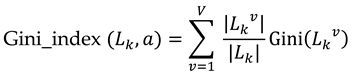
The given training data set is composed of observed random vectors (X,Y) with n instances. where the vector is a predictor or an explanatory variable with p attributes; is the class label or digital response. The principle of random forest is to randomly select k independent and identically distributed sample sets (each sample set contains n instances) from the learning sample L by using the Bagging method, and randomly select m ( m ≤ p ) attributes from the p sample attributes in each sample set to construct a decision tree, which is composed of k decision trees [43] (Figure 1). Using Bagging method has the following advantages. When random attributes are needed, Bagging method can improve performance. Moreover, Bagging can be used to continuously estimate the generalization error of the combined tree set, as well as to estimate the strength and correlation, which are performed by the Out-of-bag data [44].
In this paper, the decision tree is constructed by using the Gini index to select the partition attributes. The purity of the dataset can be defined by the Gini value:
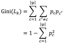 where is the proportion of c−class samples in the dataset . reflects the probability that two samples are randomly selected from the data set , and their category labels are inconsistent, that is, the smaller the , the higher the purity of the data set . The Gini index of attribute a is defined as:
 where V is the value of discrete attribute a. In the candidate attribute set m, the attribute with the smallest Gini index is selected as the optimal partition attribute, that is, .
3.2.1. Undersampling method
UnderSampling method is to eliminate the harm of skewed distribution by discarding the intrinsic samples of most classes. The simplest but most effective method is Random UnderSampling. That is, randomly selecting samples matching the number of minority classes from most classes for training, but it will involve randomly eliminating the examples of most classes, resulting in the loss of important information. Liu et al [45] proposed Easy Ensemble 's under-sampling method in 2009, that is, multiple subsets are independently extracted from most cases, and a classifier is established for each subset. Then Adaboost is used to combine all the generated classifiers to make the final decision, and the experimental results show that the method has strong generalization ability. Based on this idea, this paper proposes Ensemble Random Undersampling based on random sampling method, that is, a training data set is established by random sampling from the majority class samples many times without putting back, and the machine learning algorithm is used as the base learner for training. Finally, the prediction results are integrated. The advantage is that when the number of cycles is enough, all samples have the opportunity to participate in the training, and the integrated model will contain more information than a single subset.
The pseudo-code of the binary classification problem is as follows:
| Algorithm: Ensemble under-sampling |
| Input: The training sample is the majority class sample, is the minority class sample; |
| Base learner |
| Training rounds T. |
| Output : Integrated model N. |
| Process : |
| 1: for t=1,2,…,T do |
| 2: The subset is randomly selected from , and the size of the subset is consistent with |
| 3: We use the base learner to train a single model on the dataset : |
| 4: end for |
| 5: Integration of results |
3.2.2. Performance evaluation parameters
The results of the metallogenic prediction model based on the random forest algorithm can be represented by the Confusion Matrix (Table 1) [46]. Among them, TP and FP are the number of true/false positive samples, TN and FN are the number of true/false negative samples, respectively. In the mineral prediction, the prospective area is positive, and the non-prospective area is negative. When there is a grade imbalance or cost inequality, the error rate is not a suitable evaluation criterion. Therefore, this paper uses G-mean [47] and the area under the ROC curve AUC [48] as performance evaluation indicators, defined in equation (3)-(6).
AUC has been shown to be a reliable performance indicator for measuring imbalance and cost-sensitive problems. For a given binary classification problem, the ROC curve describes the performance using false positive ratio ( FPR ) and true positive ratio ( TPR ), where TPR is plotted on the Y axis and FPR is plotted on the X axis. The ROC curve describes the relative trade-off between gains (true positive) and losses (false positive). AUC is the area under the line, which combines the performance of the classification method of all possible values of FPR.
3.2.3. Hold-out test
A model is very important to its predictive ability in the new sample, so it is often not enough to evaluate its fitting ability only on the original data set. It is also necessary to evaluate the generalization ability of the model, that is, to evaluate the predictive ability of the model to the new sample (test set). In this paper, the data is divided into training set and test set by using the method of leaving out. 80 % of the data is used to train the model, and the obtained model is predicted on the test set of 20% data. The accuracy of the model is evaluated, and the corresponding ROC curve and AUC value are obtained.
4. Metallogenic prediction and target area delineation of Au polymetallic deposits
4.1. Geochemical characteristics of different geological units
When using stream sediments to express the geochemical characteristics of the strata, in order to understand the distribution and distribution characteristics of the elements in this area, the average values of the whole region and each geological unit are counted to reflect the content variation characteristics of the elements in this area. The coefficient of variation is used to reflect the relative dispersion degree between different elements, and the regional concentration coefficient (the average value of the elements in the geological unit / the average value of the elements in the whole area) is used to reflect the enrichment and dilution degree of the elements in the geological unit. This parameter is also called contrast, greater than 1.2 is considered to be enriched, less than 0.8 is considered to be depleted. The average value, standard deviation and coefficient of variation of stream sediment samples in each geological unit are listed in the following table, and the Great Wall system, Permian system, Triassic system, Paleogene system and Neogene system which may be related to mineralization are discussed.
4.1.1. Great Wall System (Ch)
It can be seen from Table 2 that compared with the whole area, the relatively enriched elements (including oxides) are Au (1.9) and Sn (1.3), which are a set of elements closely associated with Au and some elements related to granite. The relatively depleted elements are elements (including oxides) : Ba (0.7), Co (0.7), Mn (0.7), Fe2O3 (0.7), and the iron group elements are depleted, indicating that the basic ultrabasic rocks in the strata are not developed.

Table 2.
Geochemical characteristic parameter table of stream sediment elements in geological units.
Table 2.
Geochemical characteristic parameter table of stream sediment elements in geological units.
| Geological | N | E | K | J | T | P | C | Ch | Whole Area | |
|---|---|---|---|---|---|---|---|---|---|---|
| Unit Parameter |
||||||||||
| Au | Mean Value | 1.0 | 1.1 | 0.6 | 0.7 | 0.8 | 1.1 | 1.6 | 2.1 | 1.1 |
| Standard Deviation | 0.8 | 1.2 | 0.4 | 0.7 | 0.6 | 2.2 | 1.6 | 2.8 | 1.5 | |
| Coefficient of Cariation | 0.8 | 1.1 | 0.7 | 0.9 | 0.8 | 2.0 | 1.0 | 1.2 | 1.4 | |
| ConcentrationCoefficient | 0.9 | 1.0 | 0.5 | 0.7 | 0.7 | 1.0 | 1.4 | 1.9 | 1.0 | |
| Ba | Mean Value | 639.6 | 756.5 | 677.9 | 1598.3 | 793.9 | 580.1 | 526.3 | 513.9 | 766.7 |
| Standard Deviation | 502.1 | 531.1 | 130.1 | 6135.3 | 1776.1 | 326.5 | 219.6 | 95.3 | 2307.8 | |
| Coefficient of Cariation | 0.8 | 0.7 | 0.2 | 3.8 | 2.2 | 0.5 | 0.4 | 0.1 | 3.0 | |
| ConcentrationCoefficient | 0.8 | 1.0 | 0.9 | 2.0 | 1.0 | 0.7 | 0.6 | 0.6 | 1.0 | |
| Bi | Mean Value | 0.3 | 0.2 | 0.2 | 0.2 | 0.2 | 0.2 | 0.2 | 0.2 | 0.2 |
| Standard Deviation | 0.4 | 0.1 | 0.1 | 0.1 | 0.1 | 0.1 | 0.1 | 0.1 | 0.2 | |
| Coefficient of Cariation | 1.1 | 0.5 | 0.2 | 0.5 | 0.3 | 0.7 | 0.5 | 0.4 | 1.0 | |
| ConcentrationCoefficient | 1.5 | 1.0 | 0.5 | 1.0 | 1.0 | 1.0 | 1.0 | 1.0 | 1.0 | |
| Co | Mean Value | 11.6 | 9.7 | 7.6 | 8.9 | 12.1 | 10.7 | 10.1 | 7.8 | 10.7 |
| Standard Deviation | 3.0 | 4.5 | 2.2 | 3.9 | 3.1 | 3.6 | 3.6 | 3.3 | 4.3 | |
| Coefficient of Cariation | 0.3 | 0.5 | 0.3 | 0.4 | 0.2 | 0.3 | 0.3 | 0.4 | 0.4 | |
| ConcentrationCoefficient | 1.1 | 0.9 | 0.7 | 0.8 | 1.1 | 0.9 | 0.9 | 0.7 | 1.0 | |
| Cu | Mean Value | 21.5 | 21.5 | 18.7 | 25.2 | 26.6 | 20.7 | 27.6 | 28.2 | 24.4 |
| Standard Deviation | 4.9 | 9.8 | 3.8 | 9.9 | 8.9 | 7.4 | 16.6 | 22.7 | 11.1 | |
| Coefficient of Cariation | 0.2 | 0.5 | 0.2 | 0.3 | 0.3 | 0.3 | 0.6 | 0.7 | 0.4 | |
| ConcentrationCoefficient | 0.9 | 0.9 | 0.8 | 1.0 | 1.1 | 0.8 | 1.1 | 1.1 | 1.0 | |
| Fe | Mean Value | 4.7 | 3.7 | 3.1 | 4.3 | 5.2 | 4.4 | 4.0 | 3.1 | 4.4 |
| Standard Deviation | 1.2 | 1.7 | 0.7 | 1.8 | 1.4 | 1.4 | 1.3 | 1.0 | 1.7 | |
| Coefficient of Cariation | 0.3 | 0.5 | 0.2 | 0.4 | 0.2 | 0.3 | 0.3 | 0.3 | 0.4 | |
| ConcentrationCoefficient | 1.1 | 0.8 | 0.7 | 0.9 | 1.1 | 1.0 | 0.9 | 0.7 | 1.0 | |
| Mg | Mean Value | 1.3 | 1.6 | 1.2 | 1.4 | 1.7 | 1.6 | 2.0 | 1.6 | 1.7 |
| Standard Deviation | 0.4 | 0.8 | 0.4 | 0.6 | 0.3 | 0.4 | 0.7 | 1.0 | 0.8 | |
| Coefficient of Cariation | 0.3 | 0.5 | 0.3 | 0.4 | 0.2 | 0.3 | 0.3 | 0.6 | 0.5 | |
| ConcentrationCoefficient | 0.8 | 0.9 | 0.7 | 0.8 | 1.0 | 0.9 | 1.1 | 0.9 | 1.0 | |
| Sn | Mean Value | 2.7 | 1.8 | 1.4 | 1.7 | 2.1 | 2.1 | 2.1 | 2.9 | 2.3 |
| Standard Deviation | 1.3 | 0.8 | 0.2 | 0.5 | 0.8 | 1.0 | 0.7 | 1.0 | 2.0 | |
| Coefficient of Cariation | 0.5 | 0.4 | 0.1 | 0.3 | 0.4 | 0.4 | 0.3 | 0.3 | 0.9 | |
| ConcentrationCoefficient | 1.2 | 0.8 | 0.6 | 0.7 | 0.9 | 0.9 | 0.9 | 1.2 | 1.0 | |
| Ti | Mean Value | 3160.2 | 2395.3 | 1861.3 | 1880.9 | 2805.9 | 2515.4 | 2509.1 | 2244.3 | 2574.3 |
| Standard Deviation | 1840.7 | 979.1 | 676.5 | 875.1 | 939.3 | 967.3 | 795.5 | 631.9 | 1162.0 | |
| Coefficient of Cariation | 0.5 | 0.4 | 0.3 | 0.4 | 0.3 | 0.4 | 0.3 | 0.3 | 0.4 | |
| ConcentrationCoefficient | 1.2 | 0.9 | 0.7 | 0.7 | 1.0 | 1.0 | 1.0 | 0.9 | 1.0 |
Note: Content unit : Fe is Fe2O3, Mg is Mgo, oxide is %, other elements is ×10−6; Ch is Great Wall System;. C is Carboniferous; P is Permian; T is Triassic; J is Jurassic; K is Cretaceous; E is Paleogene; N is Neogene.
Table 2.
Geochemical characteristic parameter table of stream sediment elements in geological units.
Table 2.
Geochemical characteristic parameter table of stream sediment elements in geological units.
| Geological | N | E | K | J | T | P | C | Ch | Whole Area | |
|---|---|---|---|---|---|---|---|---|---|---|
| Unit Parameter |
||||||||||
| V | Mean Value | 65.4 | 60.8 | 53.4 | 49.5 | 64.0 | 59.3 | 71.1 | 55.0 | 63.1 |
| Standard Deviation | 19.8 | 25.4 | 22.1 | 18.2 | 17.5 | 22.7 | 26.2 | 32.9 | 25.8 | |
| Coefficient of Cariation | 0.3 | 0.4 | 0.4 | 0.3 | 0.2 | 0.4 | 0.3 | 0.6 | 0.4 | |
| ConcentrationCoefficient | 1.0 | 0.9 | 0.8 | 0.7 | 1.0 | 0.9 | 1.1 | 0.9 | 1.0 | |
| Pb | Mean Value | 20.5 | 15.2 | 14.8 | 17.6 | 21.8 | 19.2 | 15.3 | 15.6 | 18.4 |
| Standard Deviation | 5.6 | 21.3 | 3.4 | 13.5 | 21.9 | 7.6 | 5.4 | 3.2 | 15.1 | |
| Coefficient of Cariation | 0.3 | 1.4 | 0.2 | 0.7 | 1.0 | 0.4 | 0.3 | 0.2 | 0.8 | |
| ConcentrationCoefficient | 1.1 | 0.8 | 0.8 | 0.9 | 1.1 | 1.0 | 0.8 | 0.8 | 1.0 | |
| Zn | Mean Value | 68.9 | 50.1 | 46.1 | 64.6 | 78.3 | 65.5 | 64.8 | 60.0 | 66.0 |
| Standard Deviation | 18.2 | 22.7 | 11.9 | 79.3 | 65.0 | 25.6 | 21.5 | 24.1 | 48.6 | |
| Coefficient of Cariation | 0.3 | 0.4 | 0.2 | 1.2 | 0.8 | 0.4 | 0.3 | 0.4 | 0.7 | |
| ConcentrationCoefficient | 1.0 | 0.7 | 0.7 | 0.9 | 1.1 | 1.0 | 0.9 | 0.9 | 1.0 |
Note : Content unit : Fe is Fe2O3, Mg is Mgo, oxide is %, other elements is ×10−6; Ch is Great Wall System; C is Carboniferous; P is Permian; T is Triassic; J is Jurassic; K is Cretaceous; E is Paleogene; N is Neogene.
From the coefficient of variation, Au (1.3) and Cu (0.8) are extremely uneven and strongly differentiated elements, which are likely to be locally mineralized. Ba (0.2) and Pb (0.2) are evenly distributed in the strata, and there is no metallogenic basis.
4.1.2. Permian System (P)
There are no relatively depleted elements (including oxides). It is almost consistent with the level of element content in the whole region. From the coefficient of variation, Au (2.0) is a strongly differentiated element, which may be locally mineralized, and other elements are evenly distributed.
4.1.3. Triassic System (T)
The relatively depleted element is only Au (0.7), and other elements are evenly distributed. It shows that the element content in the stratum is close to the average level of the whole area.
From the coefficient of variation, Au (0.8), Ba (2.2), Pb (1.0) and Zn (0.8) are strongly differentiated elements, which have the possibility of mineralization. MgO (0.2) is an undivided element.
4.1.4. Paleogene System (E)
There is no relatively enriched element (including oxides), and the relatively depleted element is Zn (0.8).
From the coefficient of variation, Au (1.08) and Pb (1.40) are strongly differentiated elements, which may be partially mineralized.
4.1.5. Neogene System (N)
The relatively enriched elements (including oxides) are Ti (1.2). The relatively depleted element is MgO (0.8).
From the coefficient of variation, Au (0.8) and Ba (0.8) are strongly differentiated elements, which have great metallogenic possibility. Cu (0.2) belongs to the undivided elements.
4.2. Data preprocessing and data set establishment
4.2.1. Evidence layer information extraction
The data used in this paper include 1:200000 regional geological map (strata, faults, mineral distribution) and 1:200000 stream sediment geochemical data. The data analysis, processing and extraction are as follows.
(1) Stratum
According to the geochemical characteristics of the geological units in 4.1, it is concluded that the Great Wall system, Permian system, Triassic system, Paleogene system and Neogene system are the strata closely related to mineralization in the study area. The known ore spots also correspond well with these strata, so these five strata are selected respectively, and a multi-ring buffer zone with a distance of 500 meters and 10 rings is established (Figure 2).
(2) Regional fracture structure
The deep faults of different natures in different periods in the study area are very developed. The multi-stage and multi-stage magmatic hydrothermal activities and the distribution of related ophiolitic mélange belts provide favorable geological conditions for the enrichment/depletion of elements. As an important basis for regional prospecting, this paper selects the main ore-controlling fault structure as the evidence layer, and establishes a multi-ring buffer zone with a spacing of 500 meters and 10 rings (Figure 2).
(3) Regional geochemistry
The results of factor analysis showed that 4 factors with eigenvalues ≥ 1 were extracted, and the cumulative variance contribution rate was 75.58% (Table 3). The factor loading matrix was rotated using the Kaiser normalized maximum variance method, and each factor score for each sample was calculated. The eigenvalue represents the variance of the factor, which highlights the importance of the factor.
For factor 1, the variance explanation rate of the Co-V-Ti-Fe2O3-MgO-Cu group was 38.75%; this element group is linked to the suture movement of the Carboniferous-Permian plate in the Central Kunlun area and is associated with the outcropping of ultramafic and mafic rocks, mafic intrusive rocks, mafic volcanic rocks and ophiolite belts; the observed anomalies correspond well to the Carboniferous–Permian ophiolite belt [49,50,51].
For factor 2, the variance explanation rate of the Pb–Zn group was 15.44%; this result may have been related to medium–moderate and medium–high temperature hydrothermal mineralization [52], reflecting the mineralization of these elements in the Central Kunlun area. Yesanggang east lead ore, and Hongyu lead and zinc ore deposits have been found in the study area.
For factor 3, the variance explanation rate of the Bi-Sn-Au group was 13.01%, reflecting the contribution of the gold element mineralization group in the study area [53,54]. Liuzonggou and Hanzhugou placer gold deposits have been found in the area. Sn and Bi are mainly related to high-temperature volcanic hydrothermal activity, and as Bi is associated with a combination of the characteristic indicator elements of the tailing halo of gold deposits, it is often closely associated with Au.
For factor 4, the variance explanation rate of Ba was 8.39%. In addition, barite has been found in the sedimentary rocks in the eastern part of the study area, a result of Ba mineralization [55].
In order to express the results of factor analysis more intuitively, factors 2, 3 and 4 are combined into one factor, and these two main factors are extracted manually. The twelve target elements are divided into two main factors. Factor one, Co, V, Ti, Fe2O3, MgO and Cu are a group of background elements closely related to regional geological background. Pb, Zn, Bi, Sn, Au, Ba are potential ore-forming element combinations with metallogenic prospects. Among them, Pb-Zn element combination is related to medium-temperature and medium-high temperature hydrothermal mineralization. Bi-Sn-Au is related to gold mineralization in the area; Ba is closely related to the common barite mineralization in the area. Therefore, the extraction factor two is reclassified by the classification number of 10, and the Kriging interpolation method is used as one of the evidence layers of this training prediction (Figure 3).
Combined with the existing geological and regional geochemical data, and based on the above analysis and processing, seven evidence layers were finally selected for the prediction and evaluation of mineral resources prospect of gold polymetallic deposits in the central Kunlun area of Xinjiang: (1) Great Wall strata, (2) Permian strata, (3) Triassic strata, (4) Paleogene strata, (5) Neogene strata, (6) regional fault structure, (7) factor score of regional geochemical data PCA2.
4.2.2. Establishment of data sets
There are a series of practical difficulties in the application of machine learning in mineral prediction, such as the imbalance of label data (mineralization exists or not) [31]. At present, more than 20 large and small deposits have been found in the central Kunlun area of Xinjiang, and few specific locations of non-deposit areas containing different information have been marked, and there is a problem of obvious imbalance of label data. Therefore, the researchers selected 27 gold polymetallic ore deposits and 10 non-prospective ore locations from the region, extracted the input evidence layer values, and created a training data set. Each training data consists of a set of input feature vectors and a binary classification value, where 1 is a metallogenic prospect and 0 is a non-metallogenic prospect. The prediction data set is stream sediment grid data points. Due to the obvious data imbalance problem in the training data set, this paper uses two undersampling methods for comparative study. One is to use the integrated random undersampling method mentioned above for sampling. Second, by fully considering the geological factors, the typical representative known ore points are selected. The two are verified and evaluated by the leave-out method and the model performance evaluation parameters. Finally, the metallogenic prediction results of these two different undersampling methods are evaluated.
4.3. Random forest algorithm implementation
4.3.1. Parameter optimization
The parameterization of random forest has a great influence on its robustness and generalization ability, which affects the accuracy of mineral prediction. The size and depth of the random forest tree are crucial to the performance of machine learning. Too large or too small may lead to unsatisfactory results.
Unlike most machine learning methods, the random forest generation prediction model only needs to set two important parameters : the number of decision trees (Trees) and the number of evidence features that each node uses to make the decision tree grow (m). Breiman [42] proved that with the increase of Trees, the generalization error is always convergent, and there is no overfitting problem in overtraining. On the other hand, reducing the number of m will lead to a decrease in the correlation between trees, thereby improving the accuracy of the model. In order to optimize these parameters, a large number of experiments were carried out using different numbers of trees and feature numbers. The value range of Trees was set to 2 to 6, and the interval was 1. The number of feature variables m was 2, 3, and 4, respectively. The results show (Figure 4, Table 4), the average RF accuracy is 0.85, the standard deviation is 0.16, and it has high accuracy and stability. It can be seen that RF is less sensitive to parameter changes. The stable performance of RF is mainly attributed to the combination of multiple classifiers trained under certain conditions. On the one hand, the evidence features used for tree induction are randomly selected, which reduces the correlation between individual models, reduces the generalization error, and provides a very stable prediction. In addition, the feature selection method adds a re-sampling (Bagging) of the training data for each tree, which helps to increase the diversity of the models that make up the whole and prevents the decision tree from overfitting the data.
4.3.2. Prediction performance assessment
Random undersampling is used to sample the unbalanced data (27 ore spots, 10 non-ore spots) of the training data set to ensure that the data ratio of 0 and 1 in the new data set is approximately 1:1. Then the newly generated data set is trained and predicted by the hold-out method (80% training, 20% test), and the final prediction results are integrated. For the divided training data set and prediction data set, 15 parallel experiments were carried out by Tree taking 2-6, m taking 2,3,4, and the best results were taken. Figure 5 lists the confusion matrix of the test set prediction of the random forest model under different sampling methods. It can be seen that the number of positive and negative samples of correct classification is far more than the number of samples of wrong classification, and the model application is feasible. Based on this confusion matrix, the calculated evaluation parameters are shown in Table 5 (see Equation 3-6 for the calculation method). The random forest model shows different performance in different sampling methods.
As far as different sampling methods are concerned, the evaluation parameters of selecting representative training samples for training are higher than the results of integrated random undersampling. This is because the sampling method of selecting representative samples is to eliminate some known ore points, so as to make the training model fit better and the prediction results of the test set more accurate.
The ROC curve can evaluate the prediction performance of the high probability region, and the predicted classification results are judged by different discriminant thresholds. The area under the curve AUC value is used to evaluate the overall performance of different prediction models [56]. The RF curve under the selected training samples has a relatively high AUC value (Figure 6a), while the ROC curve under the integrated random undersampling (Figure 6b) is slightly inferior, but the overall gap is not large. This may be related to RF as an integrated model [42]. As an integrated algorithm based on decision tree as the base learner, RF ensures the independence of individual models by random sampling of training variables and samples, thereby improving the generalization ability. In the face of data changes in the random sampling process, its fitting effect is also more stable.
In short, from the above results, it can be concluded that the prediction performance parameters in the training process show that the prediction results of selecting representative training samples are better than the results of ensemble random undersampling.
4.3.3. Metallogenic prediction results
Figure 7 and Figure 8 show the prospect map of random forest metallogenic prediction under the training of integrated random undersampling and representative sample selection respectively. The predicted value of each point is expressed by 0-1 floating point value, which indicates the metallogenic probability value at this point. The areas with probabilities greater than 0.5 and 0.8 are extracted as delineated metallogenic potential areas and high potential areas, and areas below 0.5 are considered as low potential areas.
Table 6 is the statistical information of each metallogenic potential area under different sampling methods. It can be observed that the metallogenic prediction results predicted by selecting training samples have the following advantages compared with the integrated random undersampling method: (1) The number of ore spots misjudged in the low potential area is small and the proportion of ore deposits is low; (2) The number of ore spots correctly predicted in the metallogenic potential area is large and the ore-bearing ratio is high; (3) The number of ore-bearing points and the proportion of ore-bearing points in the high potential area are higher; the above results show that the machine learning training model under the method of selecting training samples has learned the complex information of the original data to a greater extent, and has been successfully applied to the metallogenic prediction results and prospect division.
From the above metallogenic prospect prediction and metallogenic potential division results, it can be concluded that the selection of training sample method is more reliable than the integrated random undersampling method in the metallogenic potential area due to the large number of accurately predicted ore spots and the high proportion of ore content per unit area.
5. Conclusion
Based on the previous research results, the researchers applied the random forest algorithm under different sampling methods for the first time to predict and delineate the 12 target elements of 3076 stream sediments collected by the medium-small scale regional geochemical exploration in the central Kunlun area of Xinjiang. It provides a basis for the future medium-small scale metallogenic elements from qualitative identification to quantitative prediction, and discusses the prediction effect of random forest algorithm on gold polymetallic minerals in the central Kunlun area of Xinjiang under different sampling methods. The main conclusions are as follows:
(1) In this study, the strata, fault structure and geochemical information are extracted, and the known ore spots and geochemical data are used to form a training set and a prediction set to construct a random forest model. The difference between the integrated random undersampling method and the selection of training sample method is compared, which expands the prospecting idea of machine learning algorithm in mathematical geology in the central Kunlun area of Xinjiang.
(2) For different sampling methods, the performance evaluation parameters of the training process show that the prediction accuracy of the selected training samples is higher, indicating that the fitting effect and generalization ability are stronger. Ensemble random undersampling can weaken the difference between the base learners and achieve the consistency of the overall results. The results of metallogenic prospect prediction and potential area division better explain this.
(3) The sampling method of selecting training samples is more reliable because it can fully learn the complex information of the original data, the number of ore spots accurately predicted by the prediction results is more, and the proportion of ore is higher. For the random forest model of different sampling methods, the random forest algorithm under the selected training samples has more reference value and further exploration significance in the actual exploration problems considering the cost because of its small area of high potential prediction area and high proportion of ore per unit area.
Author Contributions
Conceptualization, Y.Z. and S.X.; methodology, Y.Z. and S.X.; software, Y.Z; J.D. and X.Z.; validation, Y.Z. and S.X.; formal analysis, Y.Z.; data curation, Y.Z. and X.Y.; writing—original draft preparation, Y.Z.; writing—review and editing, Y.Z. and S.X.; visualization, Y.Z; X.Z. and X.Y.; supervision, Y.Z; S.X. and X.Z.; project administration, Y.Z.; funding acquisition, S.X. All authors have read and agreed to the published version of the manuscript.
Funding
This research was financially supported by funds from the National Natural Science Key Fund Project (71132008), Northwestern Basic Geological Survey and Data Update Project of China Geological Survey (1212010911051), Natural Science Key Project of Inner Mongolia Education Department (NJZZ11067) and Inner Mongolia Natural Science Foundation (2015BS0702).
Data Availability Statement
Not applicable.
Acknowledgments
We are very thankful for all the editors and reviewers who have helped us improve the manuscript.
Conflicts of Interest
The authors declare no conflict of interest.
References
- Kong, W.H.; Xiao, K.Y.; Chen, J.P.; Sun, L.; Li, N. A combined prediction method for reducing prediction uncertainty in the quantitative mineral resources prediction. Earth Science Frontiers. 2021, 28, 128–138, (In Chinese with English abstract). [Google Scholar] [CrossRef]
- Liu, G.; Wang, Y.Z.; Xue, T.; Wu, C.Y.; Xue, B.; Tang, T.T.; Liu, S.M. Mineral Resource Spatial Association Analysis and Prediction: A Case Study in Western China. Geoscience 2019, 33, 751–758, (In Chinese with English abstract). [Google Scholar] [CrossRef]
- Agterberg, F.; Kelly, A. Geomathematical methods for use in prospecting. Canadian Mining Journal. 1971, 5, 61–72. [Google Scholar]
- Griffiths, J.; Menzie, D.; Labovitz, M. Exploration for and evaluation of natural resources. AAPG Research Symposium, Probability Methods in Oil Exploration, Aug. 1975, 20-22.
- Singer, D.A. RESIN, a FORTRAN IV program for determining the area of influence of samples or drill holes in resource target search. Computers & Geosciences. 1976, 2, 249–260. [Google Scholar] [CrossRef]
- Singer, D.A. Basic concepts in three-part quantitative assessments of undiscovered mineral resources. Nonrenewable Resources. 1993, 2, 69–81. [Google Scholar] [CrossRef]
- Singer, D.A. Progress in integrated quantitative mineral resource assessments. Ore Geology Reviews. 2010, 3, 242–250. [Google Scholar] [CrossRef]
- Wu, D.C.; Lu, W.Q.; Wang, G.P. 3D geological modeling and metallogenic prediction of Yimaquan M14 magnetic anomaly area in Geermu City of Qinghai. Mineral Resources and Geology 2023, 37, 55–61+71, (In Chinese with English abstract). [Google Scholar] [CrossRef]
- Song, W.; Zheng, L.; Liu, J.; Cao, S.; Xie, Z. Genesis, metallogenic model, and prospecting prediction of the Nibao gold deposit in the Guizhou Province, China. Acta Geochimica. 2023, 42, 136–152. [Google Scholar] [CrossRef]
- Carranza, E.J.M.; Hale, M. Logistic Regression for Geologically Constrained Mapping of Gold Potential, Baguio District, Philippines. Exploration and Mining Geology. 2001, 3, 165–175. [Google Scholar] [CrossRef]
- Li, W.; Neubauer, F.; Liu, Y.J.; Genser, J.; Ren, S.M.; Han, G.Q.; Liang, C.Y. Paleozoic Evolution of the Qimantage Magmatic Arcs, Eastern Kunlun Mountains : Constraints from Zircon Dating of Granitoids and Modern River Sands. Journal of Asian Earth Sciences. 2013, 77, 183–202. [Google Scholar] [CrossRef]
- Seraj, R.R.R. A hybrid GIS-assisted framework to integrate Dempster-Shafer theory of evidence and fuzzy sets in risk analysis: An application in hydrocarbon exploration. Geocarto international. 2021, 36, 5a8. [Google Scholar] [CrossRef]
- Behera, S.; Panigrahi, M.K. Mineral prospectivity modelling using singularity mapping and multifractal analysis of stream sediment geochemical data from the auriferous Hutti-Maski schist belt, S. India. Ore Geology Reviews. 2021, 131, 104029. [Google Scholar] [CrossRef]
- Koike, K.; Matsuda, S.; Suzuki, T.; Ohmi, M. Neural Network-Based Estimation of Principal Metal Contents in the Hokuroku District, Northern Japan, for Exploring Kuroko-Type Deposits. Natural Resources Research. 2002, 2, 135–156. [Google Scholar] [CrossRef]
- Porwal, A.; Carranza, E.J.M.; Hale, M. Artificial Neural Networks for Mineral-Potential Mapping: A Case Study from Aravalli Province, Western India. Natural Resources Research. 2003, 3, 155–171. [Google Scholar] [CrossRef]
- Choi, S.; Moon, W.M.; Choi, S-G. Fuzzy logic fusion of W-Mo exploration data from Seobyeog-ri, Korea. Geosciences Journal. 2000, 2, 43–52. [Google Scholar] [CrossRef]
- Luo, X.; Dimitrakopoulos, R. Data-driven fuzzy analysis in quantitative mineral resource assessment. Computers & Geosciences. 2003, 1, 3–13. [Google Scholar] [CrossRef]
- Liu, Y.; Cheng, Q.M.; Xia, Q.L.; Wang, X.Q. Mineral potential mapping for tungsten polymetallic deposits in the Nanling metallogenic belt, South China. Journal of Earth Science. 2014, 4, 689–700. [Google Scholar] [CrossRef]
- Wang, W.L.; Xie, S.Y.; Carranza, E.J.M. Introduction to the thematic collection: Applications of innovations in geochemical data analysis. Geochemistry Exploration Environment Analysis. 2022, 23. [Google Scholar] [CrossRef]
- Carranza, E.J.M. Weights of Evidence Modeling of Mineral Potential: A Case Study Using Small Number of Prospects, Abra, Philippines. Natural Resources Research. 2004, 3, 173–187. [Google Scholar] [CrossRef]
- Yang, F.; Xie, S.Y.; Hao, Z.; Carranza, E.J.M.; Song, Y.; Liu, Q.; Xu, R.; Nie, L.; Han, W.; Wang, C. Geochemical Quantitative Assessment of Mineral Resource Potential in the Da Hinggan Mountains in Inner Mongolia, China. Minerals. 2022, 12, 434. [Google Scholar] [CrossRef]
- Brown, W.; Groves, D.; Gedeon, T. Use of Fuzzy Membership Input Layers to Combine Subjective Geological Knowledge and Empirical Data in a Neural Network Method for Mineral-Potential Mapping. Natural Resources Research. 2003, 3, 183–200. [Google Scholar] [CrossRef]
- Kim, Y.H.; Choe, K.U.; Ri, R.K. Application of fuzzy logic and geometric average: A Cu sulfide deposits potential mapping case study from Kapsan Basin, DPR Korea. Ore Geology Reviews 2019, 107, 239–247. [Google Scholar] [CrossRef]
- Xiao, K.Y.; Zhang, X.H.; Song, G.Y.; Chen, Z.H.; Liu, D.L.; Wang, S.L. Development of GIS-Based Mineral Resources Assessment System. Earth Science. 1999, 5, 525–528, (In Chinese with English abstract). [Google Scholar] [CrossRef]
- Cui, C.Q.; Wang, B.; Zhao, Y.X.; Wang, Q.; Sun, Z.M. China's regional sustainability assessment on mineral resources: Results from an improved analytic hierarchy process-based normal cloud model. Journal of Cleaner Production. 2019, 210, 105–120. [Google Scholar] [CrossRef]
- Karapurkar, D.D. RS and GIS based studies on Sediment yield from a tropical watershed: A case study of the Gangolli Catchment, Karnataka. Sedimentation, Tectonics, Mineral Resources and Sustainable Development.
- Xie, S.Y.; Wan, X.; Dong, J.B.; Wan, N.; Jiang, X.N.; Carranza, E.J.M.; Wang, X.Q.; Chang, L.H.; Tian, Y. Quantitative Prediction of Potential Areas Likely to Yield Se-rich and Cd-low Rice using Fuzzy Weights-of-Evidence Method. Science of the Total Environment 2023, 889, 164015. [Google Scholar] [CrossRef]
- Greff, K.; Srivastava, R.K.; Koutnik, J.; Steunebrink, B.R.; Schmidhuber, J. LSTM: A Search Space Odyssey. IEEE Transactions on Neural Networks and Learning Systems 2017, 10, 2222–2232. [Google Scholar] [CrossRef]
- Agterberg, F. Geomathematics: Theoretical Foundations, Applications and Future Developments; Springer: Canada, 2014; 552. [Google Scholar]
- Zhou, Y.Z.; Chen, S.; Zhang, Q.; Xiao, F.; Wang, S.G. Advances and Prospects of Big Data and Mathematical Geoscience. Acta Petrologica Sinica. 2018, 2, 255–263. [Google Scholar]
- Rodriguez-Galiano, V.; Sanchez-Castillo, M.; Chica-Olmo, M.; Chica-Rivas, M. Machine Learning Predictive Models for Mineral Prospectivity: An Evaluation of Neural Networks, Random Forest, Regression Trees and Support Vector Machines. Ore Geology Reviews. 2015, 71, 804–818. [Google Scholar] [CrossRef]
- Sun, T.; Chen, F.; Zhong, L.X.; Liu, W.M.; Wang, Y. GIS-based mineral prospectivity mapping using machine learning methods: A case study from Tongling ore district, eastern China. Ore Geology Reviews. 2019, 109, 26–49. [Google Scholar] [CrossRef]
- Abedi, M.; Norouzi, G.H.; Bahroudi, A. Support vector machine for multi-classification of mineral prospectivity areas. Computers & Geosciences. 2012, 46, 272–283. [Google Scholar] [CrossRef]
- Beucher, A.; Siemssen, R.; Fröjdö, S.; Österholm, P.; Martinkauppi, A.; Edén, P. Artificial Neural Network for Mapping and Characterization of Acid Sulfate Soils: Application to Sirppujoki River Catchment, Southwestern Finland. Geoderma 2015, 247-248, 38–50. [Google Scholar] [CrossRef]
- Herrera, M.; Torgo, L.; Izquierdo, J.; Pérez-García, R. Predictive models for forecasting hourly urban water demand. Journal of Hydrology 2010, 1-2, 141–150. [Google Scholar] [CrossRef]
- Xie, S.Y.; Huang, N.; Deng, J.; Wu, S.L.; Zhan, M.G.; Carranza, E.J.M.; Zhang, Y.P.; Meng, F.X. Quantitative Prediction of Prospectivity for Pb–Zn Deposits in Guangxi (China) by Back-propagation Neural Network and Fuzzy Weights-of-Evidence Modeling. Geochemistry: Exploration, Environment, Analysis 2022, 22. [Google Scholar] [CrossRef]
- Rodriguez-Galiano, V.F.; Ghimire, B.; Rogan, J.; Chica-Olmo, M.; Rigol-Sanchez, J.P. An assessment of the effectiveness of a random forest classifier for land-cover classification. ISPRS Journal of Photogrammetry and Remote Sensing. 2012, 67, 93–104. [Google Scholar] [CrossRef]
- Dong, L.H.; Zhang, L.C.; Li, W.D. Division and characteristics of geotectonic units in Xinjiang. The 6th Tianshan Geological and Mineral Resources Symposium, Urumqi, Xinjiang, China, 2008; pp. 25–32. (In Chinese). [Google Scholar]
- Pan, Y.S. Formation and Uplifting of the QingHai- Tibet Plateau. Earth Science Frontiers. 1999, 3, 153–163, (In Chinese with English abstract). [Google Scholar] [CrossRef]
- Liu, C.Y.; Liu, T. Discovery and Significance of Porphyritic Copper Mineralization in YunwuNing of XinJiang. Xinjiang Geology. 1998, 2, 185–187, (In Chinese with English abstract). [Google Scholar]
- Zhang, Y.P.; Ye, X.F.; Xie, S.Y.; Zhou, X.y.; Awadelseid, S.F.; Yaisamut, O.; Meng, F.X. Implication of multifractal analysis for quantitative evaluation of mineral resources in the Central Kunlun area, Xinjiang, China. Geochemistry: Exploration, Environment, Analysis 2022, 22, geochem2021-083. [Google Scholar] [CrossRef]
- Breiman, L. Random forests. Machine learning. 2001, 1, 5–32. [Google Scholar] [CrossRef]
- Genuer, R.; Poggi, J.-M.; Tuleau-Malot, C. Variable selection using random forests. Pattern Recognition Letters 2010, 14, 2225–2236. [Google Scholar] [CrossRef]
- Oshiro, T.M.; Perez, P.S.; Baranauskas, J.A. How Many Trees in a Random Forest? In PERNER P. Machine Learning and Data Mining in Pattern Recognition; Springer: Berlin, Heidelberg, 2012; pp. 154–168. [Google Scholar]
- Liu, T.Y. EasyEnsemble and Feature Selection for Imbalance Data Sets. 2009 International Joint Conference on Bioinformatics, Systems Biology and Intelligent Computing, Shanghai, China, 2009; IEEE; pp. 517–520. [Google Scholar]
- Xiong, Y.; Zuo, R. Effects of misclassification costs on mapping mineral prospectivity. Ore Geology Reviews 2017, 82, 1–9. [Google Scholar] [CrossRef]
- Fawcett, T. ROC Graphs: Notes and Practical Considerations for Researchers. Machine Learning 2004, 31, 1–38. https://www.researchgate.net/publication/215992134.
- Kim, E.; Kim, W.; Lee, Y. Combination of multiple classifiers for the customer’s purchase behavior prediction. Decision Support Systems. 2003, 2, 167–175. [Google Scholar] [CrossRef]
- Cui, X.L.; Liu, T.T.; Wang, W.H.; Jing, M.; Bai, Y. Characteristics of geochemistry and prospecting direction of stream sediments in Buqingshan area, East Kunlun Mountains. Geophysical and Geochemical Exploration. 2011, 35, 573–578, (in Chinese with English abstract). [Google Scholar]
- Guo, Y.; Gong, F.Z.; Ning, J.S.; Liu, Y.C.; Liu, Z. Comparative study of the content area fractal method and the traditional statistical method for determining the anomaly lower limit:a case study of Au element of stream sediment survey in Awengcuo area of Tibet. Mineral Resources and Geology. 2018, 4, 736–741, (in Chinese with English abstract). [Google Scholar]
- Thanh, T.N.; Tuyen, D.V. Identification of Multivariate Geochemical Anomalies Using Spatial Autocorrelation Analysis and Robust Statistics. Ore Geology Reviews. 2019, 111, 102985. [Google Scholar] [CrossRef]
- Feng, C.Y.; Wang, S.; Li, G.C.; Ma, S.C.; Li, D.S. Middle to Late Triassic granitoids in the Qimantage area, Qinghai Province, China: Chronology, geochemistry and metallogenic significances. Acta Petrologica Sinica. 2012, 28, 665–678, (in Chinese with English abstract). [Google Scholar]
- Guo, Z.F.; Deng, J.F.; Xu, Z.Q.; Mo, X.X.; Luo, Z.H. Late Palaeozoic-Mesozoic Intracontinental, Orogenic Process and Inter Medate-Acidic Igneous Rocks from the Eastern KunLun Mountains of North Western China. Geoscience 1998, 3, 51–59, (in Chinese with English abstract). [Google Scholar]
- Li, W.; Neubauer, F.; Liu, Y.J.; Genser, J.; Liang, C.Y. Paleozoic Evolution of the Qimantage Magmatic Arcs, Eastern Kunlun Mountains: Constraints from Zircon Dating of Granitoids and Modern River Sands. Journal of Asian Earth Sciences, 2013, 77, 183–202. [Google Scholar] [CrossRef]
- Zheng, M.T.; Zhang, L.C.; Zhu, M.T.; Li, Z.Q.; He, L.D.; Shi, Y.J.; Dong, L.H.; Feng, J. Geological characteristics, formation age and genesis of the Kalaizi Ba-Fe deposit in West Kunlun. Earth Science Frontiers. 2016, 5, 252–265, (in Chinese with English abstract). [Google Scholar] [CrossRef]
- Gribskov, M.; Robinson, N.L. Use of receiver operating characteristic (ROC) analysis to evaluate sequence matching. Computers & Chemistry, 1996, 1, 25–33. [Google Scholar] [CrossRef]
Figure 1.
Random forest algorithm flow [43].
Figure 1.
Random forest algorithm flow [43].
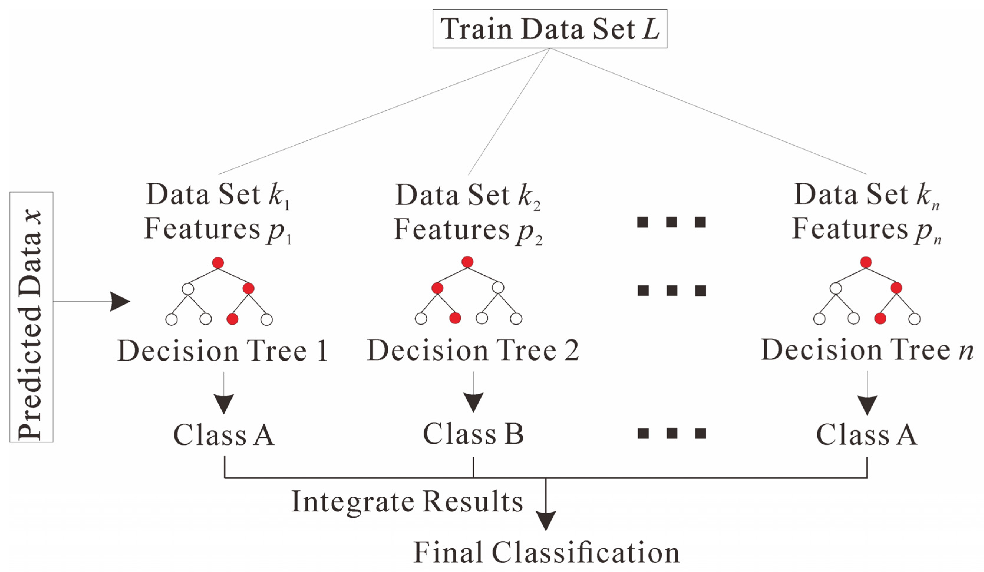
Figure 2.
Multi-ring buffer zone, (a) the Great Wall system; (b) Permian; (c) Triassic;.(d) Paleogene; (e) Neogene; (f) Faults.
Figure 2.
Multi-ring buffer zone, (a) the Great Wall system; (b) Permian; (c) Triassic;.(d) Paleogene; (e) Neogene; (f) Faults.
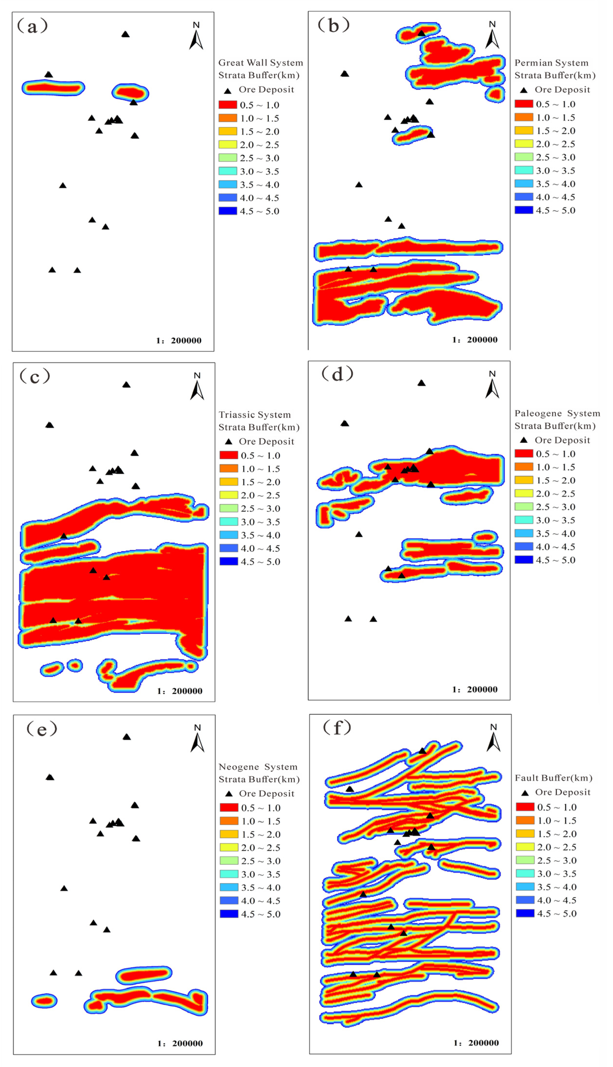
Figure 3.
PCA2 factor score plot after reclassification.
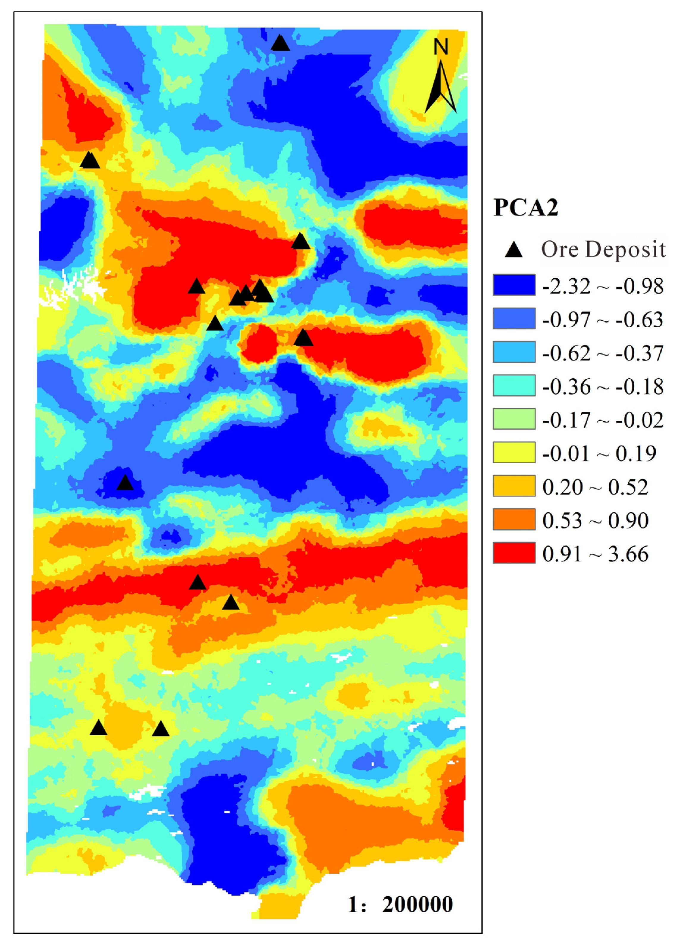
Figure 4.
Accuracy of random forest model under hyperparameters.
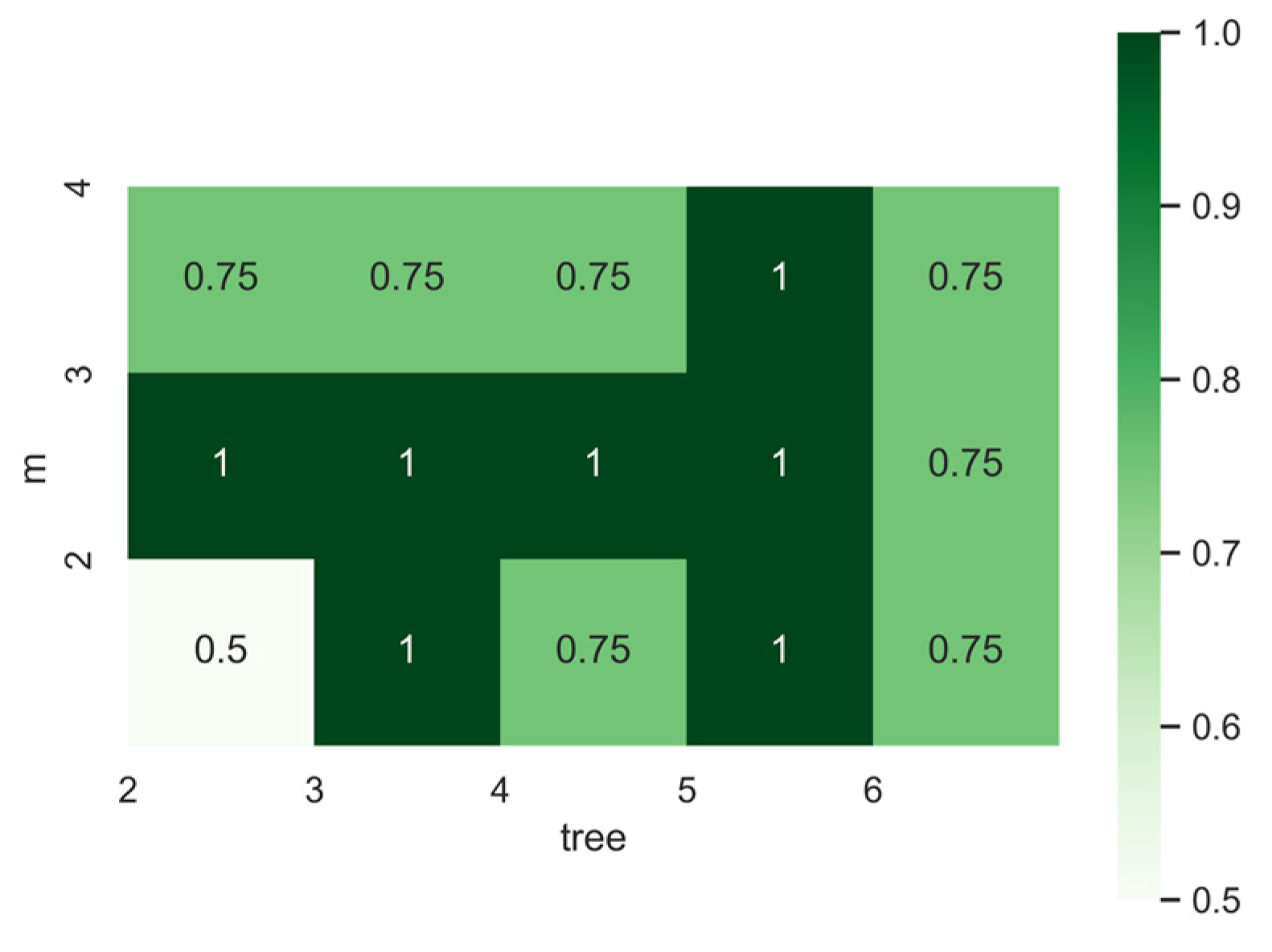
Figure 5.
The confusion matrix of random forest model under different sampling methods.
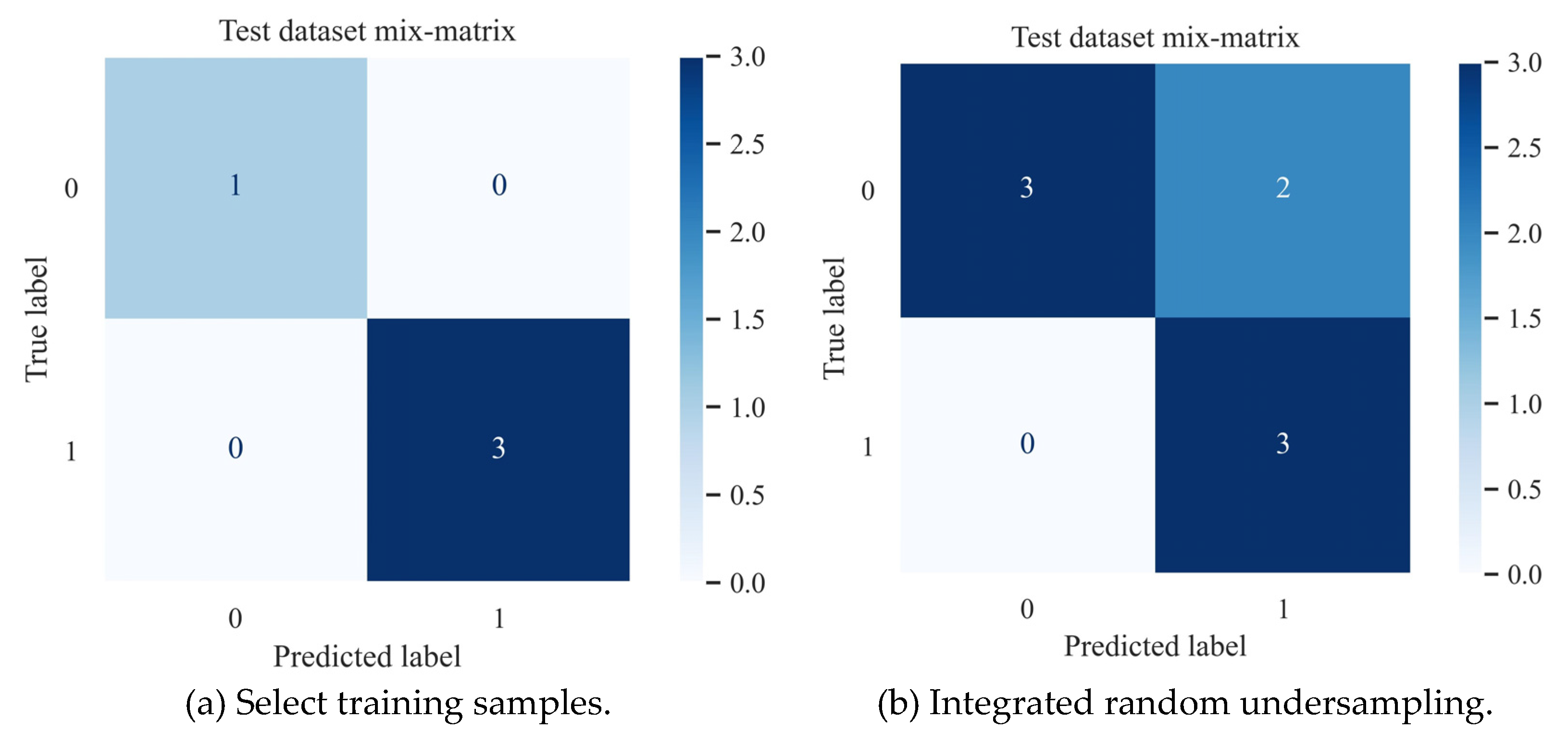
Figure 6.
ROC curve and AUC value of random forest model under different sampling methods.
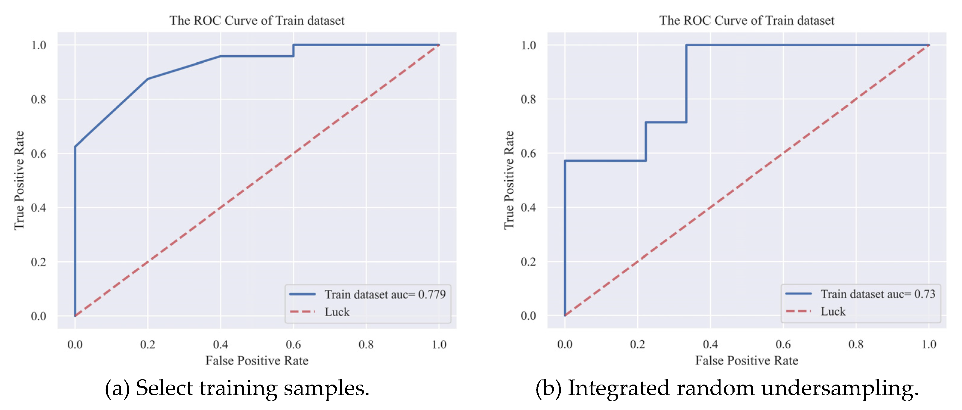
Figure 7.
Random forest metallogenic probability and metallogenic potential division.under integrated random undersampling.
Figure 7.
Random forest metallogenic probability and metallogenic potential division.under integrated random undersampling.

Figure 8.
Random forest metallogenic probability and metallogenic potential division trained by selecting representative samples.
Figure 8.
Random forest metallogenic probability and metallogenic potential division trained by selecting representative samples.
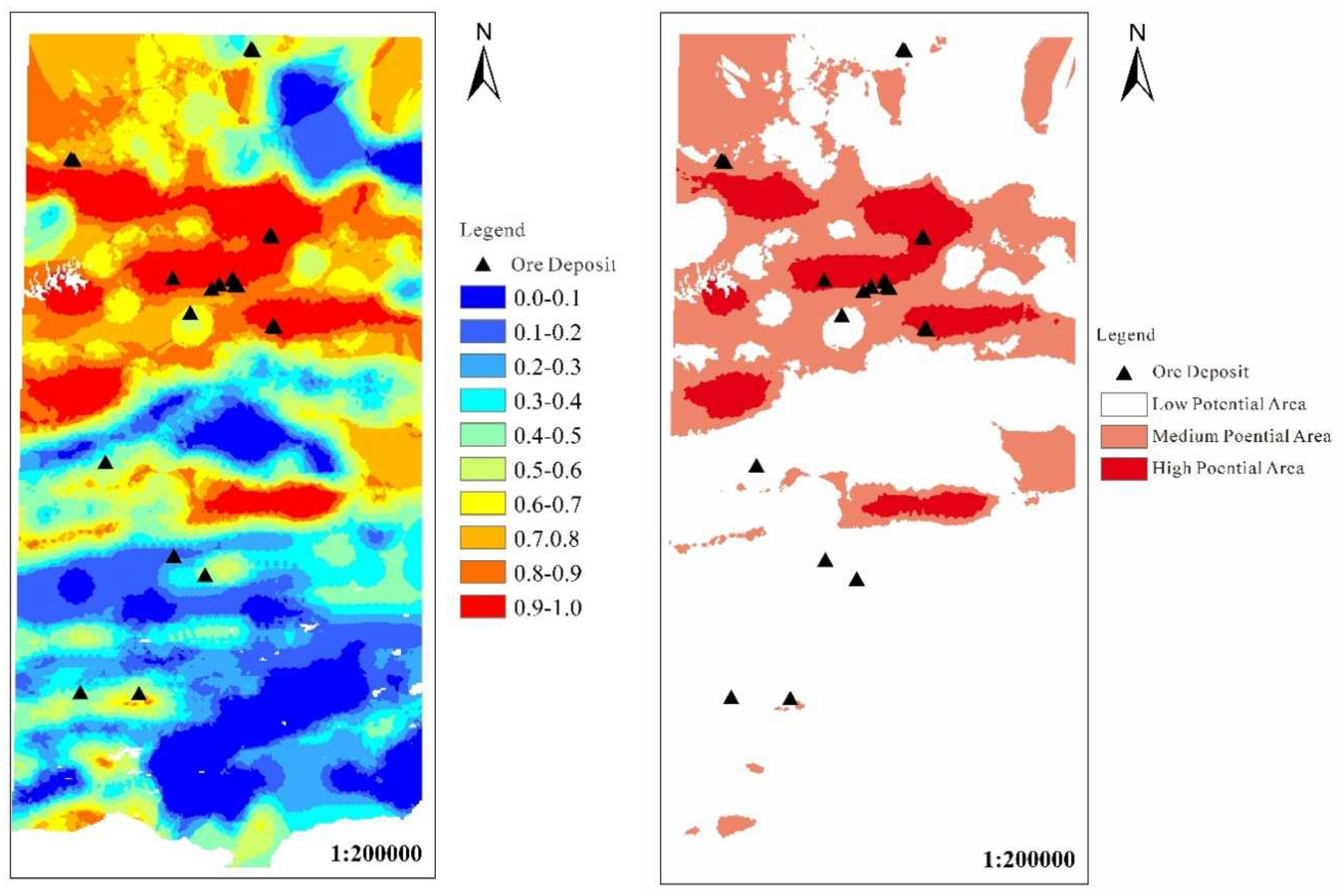
Table 1.
Confusion Matrix.
| Predicted Positive(PP) | Predicted Negative(PN) | |
|---|---|---|
| Actual Positive(AP) | TP (True Positive) | FN (False Negative) |
| Actual Negative(AN) | FP (False Positive) | TN (True Negative) |
Table 3.
Principal factor variance explanation rates derived based on the factor analysis.
| Component | Initial Eigenvalues | Rotation Sums of Squared loadings | |||||
|---|---|---|---|---|---|---|---|
| Total | % of Variance | Cumulative % | Total | % of Variance | Cumulative % | ||
| 1 | 4.65 | 38.75 | 38.75 | 4.31 | 35.91 | 35.91 | |
| 2 | 1.85 | 15.44 | 54.19 | 1.95 | 16.23 | 52.14 | |
| 3 | 1.56 | 13.01 | 67.19 | 1.80 | 15.00 | 67.14 | |
| 4 | 1.01 | 8.39 | 75.58 | 1.01 | 8.44 | 75.58 | |
| 5 | 0.92 | 7.67 | 83.25 | ||||
| 6 | 0.64 | 5.35 | 88.60 | ||||
| 7 | 0.43 | 3.61 | 92.21 | ||||
| 8 | 0.33 | 2.76 | 94.96 | ||||
| 9 | 0.27 | 2.21 | 97.18 | ||||
| 10 | 0.19 | 1.58 | 98.75 | ||||
| 11 | 0.10 | 0.81 | 99.56 | ||||
| 12 | 0.05 | 0.44 | 100.00 | ||||
Note: Factors with an eigenvalue ≥1 are selected, and Cumulative indicates the frequency at which each factor explains the total variance.
Table 4.
Hyperparameter accuracy statistics under random forest model.
| RF | |
|---|---|
| Min | 0.50 |
| Max | 1.00 |
| Mean | 0.85 |
| Std | 0.16 |
Table 5.
Prediction performance of random forest model under different sampling methods.
| Select training samples | Integrated random undersampling | |
|---|---|---|
| RF | RF | |
| Acc | 1.00 | 0.75 |
| Acc+ | 1.00 | 1.00 |
| Acc- | 1.00 | 0.60 |
| G-mean | 1.00 | 0.87 |
Table 6.
Statistical information of different metallogenic potential areas.
| Integrated random undersampling | Select training samples | ||
|---|---|---|---|
| RF | RF | ||
| Low potential areas | Known number of ore points | 7 | 5 |
| Area (km2) | 11240 | 13768 | |
| Ore-bearing ratio (%) | 0.062 | 0.036 | |
| Mineralization potential area | Known number of ore points | 9 | 10 |
| Area (km2) | 3447 | 1702 | |
| Ore-bearing ratio (%) | 0.261 | 0.588 | |
| High potential areas | Known number of ore points | 11 | 12 |
| Area (km2) | 1068 | 286 | |
| Ore-bearing ratio (%) | 1.030 | 4.196 | |
Disclaimer/Publisher’s Note: The statements, opinions and data contained in all publications are solely those of the individual author(s) and contributor(s) and not of MDPI and/or the editor(s). MDPI and/or the editor(s) disclaim responsibility for any injury to people or property resulting from any ideas, methods, instructions or products referred to in the content. |
© 2023 by the authors. Licensee MDPI, Basel, Switzerland. This article is an open access article distributed under the terms and conditions of the Creative Commons Attribution (CC BY) license (http://creativecommons.org/licenses/by/4.0/).
Copyright: This open access article is published under a Creative Commons CC BY 4.0 license, which permit the free download, distribution, and reuse, provided that the author and preprint are cited in any reuse.


