Achievable Minimally Contrastive Counterfactual Explanations

Hosein Barzekar; Susan McRoy

doi:10.20944/preprints202307.0786.v1

Preprint

Article

Achievable Minimally Contrastive Counterfactual Explanations

This version is not peer-reviewed.

This version is not peer-reviewed.

Altmetrics

Downloads

130

Views

151

Comments

Submitted:

10 July 2023

Posted:

12 July 2023

You are already at the latest version

A peer-reviewed article of this preprint also exists.

Abstract

Decision support systems based on machine learning models should be able to help users identify opportunities and threats. Popular model-agnostic explanation models can identify factors that support various predictions, answering questions like “What factors affect sales?” or “Why did sales decline?”, but do not highlight what a person should or could do to get a more desirable outcome. Counterfactual explanation approaches address intervention, and some even consider feasibility, but there has been no evaluation of their suitability for real-time applications, such as question answering. Here we address this gap by introducing a novel model-agnostic method that provides specific, feasible changes that would impact the outcomes of a complex black-box AI model for a given instance and assess its real-world utility by measuring its real-time performance and ability to find achievable changes. The method uses the instance of concern to generate high-precision explanations and then applies a secondary method to find minimally contrastive and maximally probable high-precision counterfactual explanations, while limiting contrasted features to changes that are achievable. We demonstrate that using this method, it is possible to find such explanations quickly enough for use in real-time systems. High-precision achievable minimally contrastive explanations would be useful in applications where people seek remedial actions or question how effective a proposed remedy is likely to be.

Keywords:

Machine Learning; Interpretability; Feasibility; Counterfactual and Contrastive Explanation

Subject:

Computer Science and Mathematics - Artificial Intelligence and Machine Learning

1. Introduction

Explainable AI (XAI) can serve many different aims, including increasing users’ trust in blackbox models [1] or increasing users’ understanding of how the model would behave on unseen examples [2]. One function that people would like XAI to achieve, but has yet to be adequately accomplished, is to address questions about what they can do to change the predicted outcome. This type of XAI would be useful for applications that require behavior change such as counselling, advising, or coaching, e.g., for health, education, or personal finance, where the perceived benefits of an action and the likelihood of success contribute to both initiation and ongoing maintenance of behavior change [3,4,5]. We are particularly interested in applications where people establish so-called SMART goals. SMART goals are specific, measureable, achievable, relevant, and time-bound [6]. Such goal setting would benefit from having a high-precision explanation, which is one that includes the enabling specific value for a variable, not just its name. (See Table 1 for some examples of high precision explanations.) We also prefer explanations that could be generated in real time, as part of an ongoing interaction, as this type of interaction has been shown to result in greater trust in decision support systems as compared to traditional web-based graphical user interfaces [7].

Explanations specifying instances that result in a different outcome than a given one are known as counterfactuals. Counterfactuals are the type of explanation that many people find most natural and intuitive. Indeed, research across cognitive science, philosophy and social science has found that people expect `why’ questions to be answered by explanations that are contrastive, selective, and socially interactive [8] - that is, they want answers that are solution-focused. The need for explanations that support remediation of a poor outcome has also been supported by recent user studies of XAI, which found that queries to maximize a prediction were among the top ten types of questions that people would ask of an AI model - along with more general `why’ type questions [9]. Wachter et al [10] has proposed that counterfactual and contrastive explanations (CCE) would be an effective approach to XAI and recent systematic reviews show growing interest in CCE among XAI researchers [11].

For intervention purposes, it is also important to consider the feasibility or achievability of a counterfactual [12], which means that the change would be possible through something that a person could choose to do. Finding a set of such actions is a special case of counterfactual explanation known as algorithmic recourse, which is also related to causal machine learning [13,14]. Achievability requires that there be a domain-specific action that includes the desired change as one of its effects, either directly, such as walking to change a physical activity variable, or through a change to a state of knowledge. For example, a clinician could order a diagnostic test to rule-in or rule-out the presence of a disease. Here we will presume that there is a knowledge model that provides this information, which distinguishes our approach from those that try to infer feasibility from a set of observations. Because options for recourse are often quite limited, providing such a model would not be difficult, but does raise some practical concerns. For example, when only a few changes are achievable, it is not clear how often recourse is possible, how hard it will be to find suitable recourse, or how often effective recourse can be found quickly enough for use in real-time interaction. Research on human-computer interaction has shown that the ideal latency for communicating recourse, as a form of keyboard based interaction, should be no more 200 milliseconds [15].

We propose a two step process for finding achievable counterfactuals satisfactory for real-time interaction: first find high-precision explanations of the current prediction and then find achievable changes that the AI model predicts would result in the desired outcome. If successful, this approach would allow a system to address both `why’ and `what can be done’ queries for the same scenario. From a technical standpoint, this process provides explanations that are local, model-agnostic, high precision, achievable minimally contrastive counterfactuals, concepts we shall define in detail below.

Model-agnostic explanations: address how a model performs under various conditions or inputs rather than attempting to explain the inner workings of a model. In practice, this means that the approach can be used for a variety of machine learning models, including those that do not generate rules or otherwise support interpretability [1].
Local explanations: provide justification for the behavior of a model for a particular instance, rather than all possible instances. In tabular data, as we consider here, an instance comprises a set of features, each associated with a value from a designated set of possible values, and an outcome is a discrete class, which is a feature with a known set of possible values that has been designated as the ’target’. Local, model-agnostic explanations can be found by perturbing the values of features of the given test case to identify which changes do or do not affect the target prediction [1,16].
High-precision explanations: are local explanations indicating both the features and the value or range of values for the feature sufficient to support a prediction. Anchors [2] are high-precision local explanations that include features that justify an outcome independent of the values that the other features might have.
Contrastive counterfactual explanations: are local explanations that achieve a target outcome $T_{2}$ complementary to the original outcome $T_{1}$ , by changing the value of a set of input features for an instance [17]. These features might be causally related to the outcome - but one does not need to have explicit causal information to find counterfactuals; one can achieve a good approximation using the trained AI model to formulate a prediction, given a contrastive instance [18].
Achievable contrastive counterfactual explanations: are local explanations that achieve a target outcome $T_{2}$ complementary to the original outcome $T_{1}$ , using only features whose values would be feasible for the subject of the decision system to change. This information is domain and task-specific. We assume that all features that would be feasible to change and any constraints on possible changes are provided to the system and that the system only perturbs values respecting these constraints. (For a socially interactive system, such as a conversational agent, the system should also have access to non-technical descriptions of the actions for achieving the desired value for a feature.)
Minimally contrastive counterfactual explanations: are local explanations that achieve a target outcome $T_{2}$ complementary to the original outcome $T_{1}$ , using only minimal subsets of features, such that if $M C C_{j}$ is a minimally contrastive explanation, and $M C C_{j} \equiv {m_{1}, m_{2}, \dots, m_{j}}$ then for any $m_{i} \in M C C_{j}$ , $M C C_{j} ∖ {m_{i}}$ would not be sufficient to achieve $T_{2}$ . We shall take it as obvious that people would favor making fewer changes, but preferences among changes involving different features depend on individual preferences.

2. Related Work

The most closely related work is that of Poyiadzi et al [19] who provide an algorithm for Feasible and Actionable Counterfactual Explanations (FACE). The FACE algorithm is a variant of Dijkstra’s algorithm for finding shortest paths. The FACE approach creates a graph of instances similar to a given test case. In the graph, nodes correspond to instances and edges exist between pairs of instances that differ in the value of exactly one feature if and only if it would be feasible and actionable for the anticipated user to make the corresponding change to the value of a feature, as given by a pre-specified condition function. FACE also allows one to provide a ’weight’ function to establish preferences over different types of changes. This approach provides local model-agnostic counterfactuals, but like most approaches other than anchors, this method would only return a single data point, rather than a high-precision explanation. Also, the authors do not reveal how long it might take to create or use the graph of instances for a specific dataset, given a limited set of actionable features.

Making sure that individuals have a say in how their personal lives are affected by machine learning is the main concern of "Actionable Recourse in Linear Classification" [20]. In this paper, the authors introduce the notion of `recourse’, referring to a person’s ability to influence a model’s outcome by changing `actionable’ inputs. The authors suggest using integer programming-based techniques that are optimized for redress in linear classification issues as a means of achieving this goal, but do not consider real-time performance.

Other related work is that of Mothila et al [21], which provides an approach to finding a diverse set of feasible counterfactual actions by generating a set of contrasting feasible counterexamples. Their algorithm generates new contrasting examples, while assessing a diversity metric over the generated examples. Feasibility itself is determined by the proximity approach first suggested by Wachter et al [10], which is based on proximity, rather than a domain model. Similarly, Karimi et al [12] suggest an optimization approach to find a minimal cost set of actions (in the form of structural interventions) that results in a counterfactual instance yielding the favourable output; that is, it associates costs with actions (edges) rather than features, acknowledging that not all modifications of a feature may be equally acceptable. They do not provide an explicit algorithm or implementation, but suggest using the Abduction-Action-Prediction steps proposed by Pearl [18]. Thus it is not clear under what conditions this approach might be suitable for real-time interaction.

3. Materials and Methods

The primary objective of this research is to provide a real-time, high-precision, model-agnostic method for recourse. The approach is to modify and extend the functionality of the local, model-agnostic explanation algorithm proposed in "Anchors: High-Precision Model-Agnostic Explanations" and assess its suitability for use in an interactive system. The key adaptation is to use it find minimally contrastive counterfactuals, using only achievable modifiable factors that are also anchors.

We focus on two main research questions: 1) When the set of features is reduced to include only plausibly actionable ones, how often can the anchors approach find at least one explanation that would be an effective intervention using a dataset suitable for algorithmic recourse? and 2) Under these circumstances, how quickly can we find such recourse? Secondarily, we also assess the impacts of varying the value of an internal parameter of the anchors algorithm controlling how many alternatives it keeps under consideration when trying to maximize coverage (beam size).

3.1. Algorithm for Generating Achievable Counterfactuals

In the pursuit of finding counterfactuals, our approach explores alternatives to the original instances by modifying one feature at a time and then assessing the outcome using the trained model. The primary objective of this methodology is to pinpoint a variant of a given instance that prompts a shift in the classifier’s original suboptimal prediction to a more optimal one, given the context of the domain and user preferences.

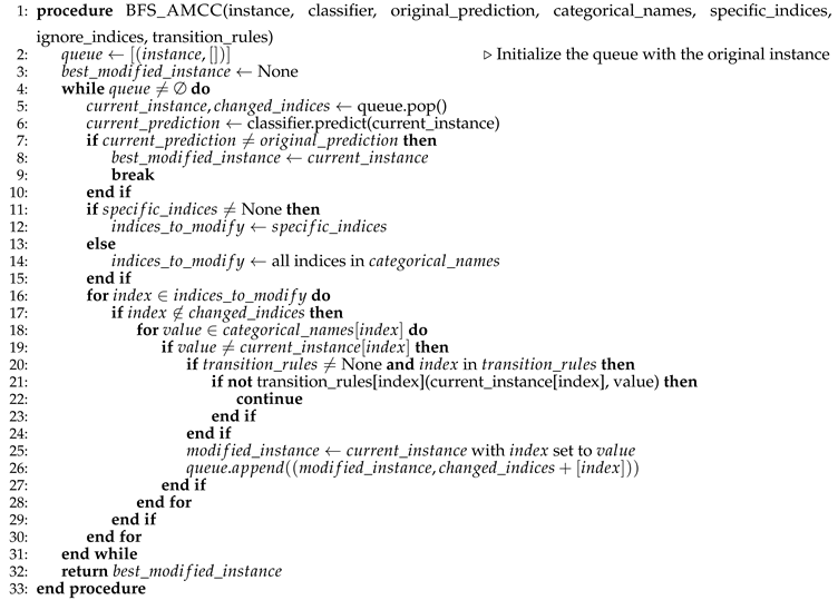
Our focus on achievable minimally contrastive counterfactuals (AMCC) led us to adopt Breadth-First Search (BFS), a graph search algorithm that explores all nodes at the current depth level before proceeding to the next. We tailored BFS to suit our objective, creating a variant termed "BFS_AMCC", as detailed in Algorithm 1.

BFS_AMCC initiates its operation by populating a queue with the original instance. During the algorithm’s core loop, an instance is dequeued for prediction. If the modified instance’s prediction deviates from the original, it is deemed a successful modification and the algorithm halts. If not, the algorithm proceeds to identify features for potential modification. In the absence of any specifically provided indices, the algorithm treats all categorical indices as modifiable.

BFS_AMCC also accommodates a set of `transition_rules` for the features. These are optional and can be used to define valid transitions between feature states, ensuring that the algorithm only considers achievable and realistic modifications to the instances. If a `transition_rule` is specified for a feature, the algorithm only considers the new feature value if the transition rule returns true when applied to the current and new feature values. These transition rules would be domain specific, ideally derived from an ontology, but for simple data can be specified directly.

In its iterative process, BFS_AMCC sifts through each index, creating a modified instance for each valid feature value perturbation and queuing it. This iteration continues until a modified instance prompts a shift in the original prediction to the desired outcome, or until the queue is exhausted.

Ultimately, BFS_AMCC returns the successfully modified instance— an achievable, minimally contrastive counterfactual that influences the classifier’s original prediction towards a preferred outcome. If no successful modification is found, the algorithm returns ’None’. This methodology guarantees the discovery of a locally minimal counterfactual, offering advanced interpretability due to its minimal feature divergence from the original instance.

Algorithm 1: BFS for achievable minimally contrastive counterfactuals to change the predicted value

3.2. Procedure for Evaluating Counterfactuals

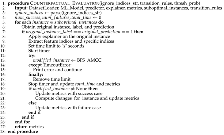
Our empirical evaluation strategy, presented as Algorithm 2, is designed to assess the performance of our approach to counterfactual generation—specifically, BFS_AMCC. The main objectives are to calculate the proportion of successful counterfactual instances and to measure the computational time required for each successful instance. These metrics are stored in a Python dictionary for analysis.

To increase the efficiency and practicality of our approach, we introduce a 10-second time limit for each instance using Python’s `signal` module. This time limit excludes extreme outliers and maintains a reasonable balance between exhaustive search and computation time. It is also very conservative, given the target for real-time interaction should be 200 milliseconds or less [15]. In practice, this time limit is rarely ever reached, usually when there is no possible recourse.

The algorithm begins by parsing the `ignore indices’ parameter, which identifies the features not to be altered during the BFS_AMCC process. It also initializes counters for successful and failed instances, along with a timer to track the computation time for each instance.

The main loop of the algorithm processes each instance in the `suboptimal_instances’ list, where instances are those classified as suboptimal by the machine learning model. For each such instance, the algorithm retrieves the true label and the classifier’s prediction.

If the classifier’s prediction matches the true value, the algorithm uses the `AnchorTabularExplainer’ to identify high-precision features. These features are then used in the BFS_AMCC process to guide the generation of modified instances.

Next, the algorithm applies the BFS_AMCC function (Algorithm 1) to generate a modified instance within the provided time limit. If a modified instance is found within this limit, the algorithm updates the success counter, records the time taken, and logs the changes. Otherwise, if a suitable counterfactual cannot be found within the time limit, a `TimeoutError’ is raised, and the algorithm moves to the next instance, increasing the failure counter.

Upon processing all instances in the `suboptimal_instances’ list, the algorithm returns the `metrics’ dictionary. This dictionary provides a comprehensive summary of the performance of our strategy, containing the number of successful and failed instances, total computation time, and a detailed log of changes for each successful counterfactual instance.

Algorithm 2: Evaluation of Counterfactual Generation

4. Experiments and Results

This section describes each of the steps in our evaluation along with their results. The evaluation assesses the difficulty in finding AMCC explanation, as both success rate and time taken, for a representative data set. We also perform preliminary experiments to create an optimal classifier and experiments where we vary a key parameter within the Anchors algorithm, `beam size’. Lastly we provide examples of the AMCC explanations that would be provided for a sample of test cases, along with their computation time.

4.1. Dataset Selection and Preparation

We selected a widely available tabular dataset, HMEQ, that appears to include several actionable features. HMEQ is from the domain of lending, where the predicted outcomes are

{G O O D, B A D}

, where a bad loan is one that resulted in a default and serious delay in repayment and a good loan was repaid on time. This dataset can be found on Kaggle.

This dataset has a total of 5,960 instances corresponding to individual home equity loans, where the adverse outcome,

f = 1

(BAD) occurs in about 20% of cases (

n =

1,189) For each applicant, 12 input variables were recorded; we determined that seven of them were actionable, as shown in Table 2, along with recourse actions for those variables. We noted several cases where transitions would likely only be desireable or achievable in one direction, and thus will treat MORTDUE, DELINQ, NINCQ, DEBTINC, as feasible to decrease, but not to increase.

Note that most of the features in HMEQ have continuous numeric values (e.g., sizes of loans, years on the job, etc.). To improve the performance for the linear models we tested, we first discretized the continuous variables into four broad categories using sklearn’s KBinDiscretizer. The exact ranges for the four categories are shown in Table 3.

After preparing the data, we assessed the difficulty of the core classification task by using the dataset to train two widely used classifiers and assessing them using standard measures (Precision, Recall, and F1).

4.2. Assessment of Classifier Performance

For this part of the evaluation, we compared RandomForest and XGBoost classifiers. RandomForest forms multiple decision trees during training, using randomly diversified input variables and data instances to enhance the model’s generalization ability. XGBoost employs a sequential gradient-boosting approach, successively building models that fix the errors of previous ones, reducing the model’s bias and improving its accuracy [22].

Implementation of these algorithms, as well as the process of generating different feature combinations, was achieved using Python and the NumPy library for efficient mathematical computations. We further harnessed Python’s native functionalities in the post-processing stage to generate contrastive anchors, evaluate changes in predictions, and prune redundant supersets.

4.3. Setup for Machine Learning Models

We initiated our empirical analysis with two machine learning models: Random Forest and XGBoost. These models were evaluated using accuracy, precision, recall, and F1-score, across train-validation-test splits of 80%-10%-10%, 70%-15%-15%, and 60%-20%-20%, as presented in Table 4.

The F1-score of the XGBoost model remained relatively steady across all splits, with a decline at a 70%-15%-15% split. In contrast, the Random Forest model improved its F1-score as the training data proportion increased, achieving the peak score of 0.75 with an 80%-10%-10% split.

Given the best F1-score was achieved by the Random Forest model, configured with an 80%-10%-10% split, this model and split were used for subsequent counterfactual evaluations.

Table 5 delineates the specific parameters used for the Random Forest and XGBoost models in these experiments. The parameter values were selected empirically to optimize the models’ performance on the training data, based on our preliminary experiments with the dataset. For the Random Forest model, we used a ’log_loss’ criterion and log2 max features with 100 estimators and 5 jobs. Similarly, the XGBoost model was configured with a ’logloss’ evaluation metric and a specific setting for tree depth, subsample by the tree, and the number of estimators.

4.4. Evaluation of the BFS_AMCC Approach

After selecting the blackbox AI model, the BFS_AMCC algorithm was systematically applied to instances initially categorized as ’BAD’ by the model. For this analysis, we treated as immutable the indices 4, 5, 6, 7, and 9 (corresponding to REASON, JOB, YOJ, DEROG, and CLAGE) and specified transition rules to prevent an increase in four variables (DEBTINC, NINQ, DELINQ, and MORTDUE). This resulted in 81 instances from the test set.

Our findings for the success rate of BFS_AMCC showed that, despite the constraints limiting actionability, the algorithm successfully found viable modifications for 38 out of 81 instances, yielding a success rate of 47%. On the other hand, the algorithm failed to find a feasible counterfactual for 43 instances within the set time limit. We excluded the top two outliers from this count, which took an unusually long processing time of 2.75 seconds (about ten times the average). These results, visualized in Figure 1, underscore the efficacy of the BFS_AMCC algorithm in finding potent, achievable modifications, even under the limitations imposed by immutable variables and transition rules.

To assess suitability for real-time use, we calculated the time taken for modifications and created a histogram. Figure 2 shows the percentage distribution of the time taken for each modification, showing that more than 90% of modifications were completed in 400 milliseconds or less, regardless of success.

We also compared the time taken for successful and unsuccessful modifications and constructed a boxplot, as shown in Figure 3. The plot shows that for both successful and unsuccessful modifications, the median times for obtaining an answer were well below 200 milliseconds, which has been found to be acceptable for conversational tasks [15]. This comparison confirms the suitable efficiency of the BFS_AMCC algorithm for use in real-time interactive systems.

4.5. Evaluation of Impact of Beam Size

Use of the anchors algorithm requires specifying `beam size,’ which is the maximum number of candidates that it will store while searching, where candidates are ordered by how well they cover the data. For the purposes of speed, a smaller beam might seem better, however, using too small a beam can lead to discarding successful candidates, causing a longer search. Since what beam size to use depends on the data and how many features are mutable, we tested a range of values for the beam, under two conditions: restrict BFS_AMCC to use only actionable features and any transition rules (Ignore indices is TRUE) or let BFS_AMCC use any anchor (Ignore indices is False).

Table 6 shows the performance of the BFS_AMCC algorithm under three different beam sizes and conditions of ignored indices with transition rules (the typical use case) versus full flexibility. The total time is the aggregate for the test set. (We consider the average for an individual case below.) Not surprisingly, the findings show that granting the algorithm complete freedom in feature manipulation, by setting both ignored indices and transition rules to FALSE, bolstered success rates across all examined beam sizes. However, this unconstrained exploration came with a high computational overhead, evidenced by a substantial increase in execution time. On the other hand, enforcing constraints via ignored indices and transition rules (the TRUE condition) resulted in a lower success rate, but yielded a significant reduction in computation time. These observations underscore the importance of careful parameter tuning (for beam size) and placing realistic constraints on feature perturbation in the optimization of BFS_AMCC. There is a delicate trade-off between success rate, computational efficiency, and the extent of allowable feature manipulations that will need to be assessed for each domain.

Table 7, shows the results when calculating the mean time for both successful and unsuccessful modifications. The results indicate that the average time taken for a successful modification is only 80 milliseconds and much shorter compared to unsuccessful ones, 190 milliseconds on average.

4.6. Examples of BFS_AMCC Modifications that Improve Predicted Outcomes

As a final assessment of the practical utility of the BFS_AMCC approach, we considered what recommendations might be provided, and how long it took to find these explanations, for a sample of test cases. Table 8 shows a collection of representative instances reflecting variable modifications and their corresponding computational times. All these changes in variable values were performed by the BFS_AMCC algorithm on instances initially classified as ’BAD’. Each row represents a unique instance with modified variable(s) and the time taken. For example, the first row illustrates a change in the ’DELINQ’ variable from 4.0 to 2.0, corresponding to a reduction of delinquent credit lines from 11–15 to the range 4–7. Finding this result took 63 milliseconds. We observed that the computational time typically remained under one second even when multiple variables were altered simultaneously, as shown in the second, fifth and seventh rows, which took 650, 150, and 210 milliseconds respectively. These findings exemplify the efficiency of the BFS_AMCC algorithm in transforming data instances while minimizing computational burden.

5. Discussion

Overall, the findings indicate that one can use BFS_AMCC to provide high precision explanations that respect the information provided, including which features are actionable and which transitions are achievable. Success rates for finding achievable minimally contrastive counterfactual explanations were comparable to finding unconstrained high precision predictions, and were found much more quickly. Across all tested beam sizes, the AMCC results took about one tenth the time for an unconstrained search, and nearly always less than 200 milliseconds. Thus our primary research questions were addressed.

We also note that careful consideration of the HMEQ dataset confirms that achievability must be specific to individual actions and transitions, in a domain specific manner. For example, while it might be achievable to reduce one’s mortgage by paying it down, one cannot feasibly increase it. (When a dataset suggests that such a change would lead to a better outcome, it is more likely an indicator that it would have been better to have been wealthy in the first place.) We address this issue by allowing one to specify transition rules. In this case, we added one so that any change with an increase to `MORTDUE’ would not be considered. Also, looking at examples shown in Table 8, some changes that our specified rules allowed might still require interaction with the user; for example, the modification CLNO (2 → 3) corresponds to increasing one’s open credit lines from 18–35 up to 36–53. The acceptability and achievability of such a change would depend on individual circumstances and possible interactions among variables that we did not consider.

We acknowledge that the specific changes reveal explanations that correspond to the information provided, and could be mentioned it a recommendation, but still might not be feasible for a particular individual in the context of the domain. For example, DELINQ: (4.0 → 2.0), corresponds to reduce the number of delinquent credit lines from as many as 15 to under 7, which might depend on the size of these debts. In a dialogue, the user could reject this suggestion and a new AMCC result created with DELINQ treated as immutable. Similarly one could address `what-about-X’ type questions by treating only X as mutable. One could also explore creating a variation of the AMCC approach that used a beam search instead of breadth-first, to return multiple candidates, ordering the candidates either by some person-specific utility or by probability of success.

Applying the algorithm to a real-world lending dataset and observing its success in altering numerous ’BAD’ instances shows its practical relevance. For example, both decision-makers and loan applicants might benefit from help identifying requisite changes for improved outcomes or discerning when no feasible recourse exists. These insights could also support educational initiatives aimed at enhancing financial literacy.

As highlighted by the distribution of successful and unsuccessful modifications shown in Figure 1, the BFS_AMCC algorithm effectively modifies a majority of instances, affirming our initial research question. Furthermore, these modifications are executed rapidly, typically within 200 milliseconds, responding to our second research query regarding the speed of recourse identification. By integrating a stringent time constraint within the BFS_AMCC, the real-time efficiency of the algorithm can be further enhanced.

Insights from Table 6 illustrate how the performance of the BFS_AMCC algorithm is influenced by variations in beam size and ignore indices conditions. It appears that an equilibrium between computational resources and algorithm performance needs to be maintained, and evaluated empirically. With ignore indices set to TRUE, consistent success rates across various beam sizes were observed, with smaller beam sizes offering enhanced efficiency. Conversely, when ignore indices was FALSE, a larger beam size led to a minor success rate increase but a significant rise in computational time. This finding underscores the importance of judiciously choosing the beam size and setting ignore indices, a conclusion further substantiated by the exclusion of top outliers under ignore indices set to FALSE.

The contrast in time taken for successful versus unsuccessful modifications (Figure 3 and Table 7) elucidates another key aspect. Despite initially seeming paradoxical, the faster completion of successful modifications can be explained by the breadth-first search nature of the BFS_AMCC algorithm, which finds achievable modifications early in the traversal. In contrast, unsuccessful modifications necessitate a more exhaustive search before concluding no successful modification exists. This suggests that in real-time use it is safe to set a time-bound and respond with the negative outcome if it is reached.

Table 8 showcases the efficiency of the BFS_AMCC algorithm in adjusting data instances. The ability to modify multiple variables simultaneously while maintaining low computational times exemplifies the optimized search and transformation capabilities of the algorithm. This highlights the algorithm’s potential for scalability and suitability in complex scenarios. Furthermore, the successful execution of transformations within certain constraints, such as immutable variables, illustrates its adaptability and versatility, broadening its potential application across diverse problem-solving domains.

Finally, the superior performance of the RandomForest classifier in our experiments emphasizes the significance of model selection in such analyses. The classifier’s ability to navigate high-dimensional feature spaces and intricate decision boundaries in the dataset may account for its success. This study offers insights into the interaction between different models and the BFS_AMCC procedure, providing a foundation for future research. For example, for datasets with large numbers of features, one might also want to consider automated feature selection.

Despite the positive findings in our evaluation of the BFS_AMCC algorithm, we recognize important limitations inherent in our study. While BFS_AMCC allows for the inclusion of immutable features via the ignore indices parameter, the process of deciding which features are mutable and to what extent, may pose challenges in real-world applications, as it requires knowledge of the domain. Additionally, establishing a suitable time-bound for instances where no feasible recourse exists, remains an interesting area for future exploration. As with many aspects of machine learning, one should conduct a systematic evaluation of alternative parameter settings.

Future research can delve more exhaustively into how different predictive models impact the BFS_AMCC procedure’s performance, how the process might be adapted to handle data with variable degrees of feature mutability, and whether there are alternative strategies for generating counterfactuals that could be as effective or potentially superior.

Even with these complexities, the findings discussed here represent a significant advance in our understanding of how to identify and utilize counterfactuals for more interpretable machine learning prediction and intervention, paving the path for further developments.

6. Conclusions

In this paper, we introduce the BFS_AMCC algorithm, a robust tool for identifying achievable, minimally contrastive counterfactuals for any machine learning framework suitable for tabular data. The ability to provide such high-precision, model-agnostic achievable counterfactuals is critical for decision support systems that use machine learning models, as it allows them to support intervention, not just prediction. In interactive settings, users who receive a negative outcome will want to ask why and what they can do to get a better outcome. A system should be able to answer them with achievable recommendations and ideally within 200 to 500 milliseconds. The findings presented here illustrate that our BFS_AMCC algorithm usually generates at least one actionable explanation that permits meaningful intervention, and it does so in an accceptable timeframe. This study therefore provides compelling evidence for the efficacy of BFS_AMCC. Moreover, the BFS_AMCC approach aligns with key requirements for real-world applications and end-user interpretability, underscoring its practical potential.

Author Contributions

Conceptualization, H.B. and S.M.; methodology, H.B. and S.M.; software, H.B.; validation, H.B. and S.M.; formal analysis, H.B.; investigation, H.B.; resources, H.B. and S.M.; data curation, H.B.; writing—original draft preparation, H.B., and S.M.; writing—review and editing, S.M; visualization, H.B.; supervision, S.M.; project administration, S.M.; funding acquisition, N/A All authors have read and agreed to the published version of the manuscript.

Funding

This research received no external funding. The authors acknowledge the support of the Office of Dean of the College of Engineering & Applied Science at the University of Wisconsin-Milwaukee.

Data Availability Statement

The data from this study is derived from the widely available Home Equity Loan Default dataset. The original dataset can be found on Kaggle at: https://www.kaggle.com/datasets/lchipham/home-equity-loan-default. https://www.kaggle.com/datasets/ajay1735/hmeq-data. For requests to used our modified data, please contact the corresponding author.

Acknowledgments

The authors thank their families for their continued patience and support.

Conflicts of Interest

The authors declare no conflict of interest. The funders had no role in the design of the study; in the collection, analyses, or interpretation of data; in the writing of the manuscript; or in the decision to publish the results.

Abbreviations

AMCC	Achievable Minimally Contrastive Counterfactual Explanation
AI	Artificial Intelligence
BFS	Breadth First Search
CCE	Contrastive Counterfactual Explanation
RF	Random Forest
XAI	Explainable Artificial Intelligence

References

Ribeiro, M.T.; Singh, S.; Guestrin, C. "Why Should I Trust You?": Explaining the Predictions of Any Classifier. In Proceedings of the 22nd ACM SIGKDD International Conference on Knowledge Discovery and Data Mining; KDD ’16; Association for Computing Machinery: New York, NY, USA, 2016; pp. 1135–1144. [Google Scholar] [CrossRef]
Ribeiro, M.T.; Singh, S.; Guestrin, C. Anchors: High-Precision Model-Agnostic Explanations. In Proceedings of the AAAI Conference on Artificial Intelligence (AAAI); 2018. [Google Scholar]
Deci, E.L.; Ryan, R.M. The" what" and" why" of goal pursuits: Human needs and the self-determination of behavior. Psychological Inquiry 2000, 11, 227–268. [Google Scholar] [CrossRef]
Ryan, R.M.; Deci, E.L. Self-determination theory and the facilitation of intrinsic motivation, social development, and well-being. American Psychologist 2000, 55, 68. [Google Scholar] [CrossRef] [PubMed]
Kwasnicka, D.; Dombrowski, S.U.; White, M.; Sniehotta, F. Theoretical explanations for maintenance of behaviour change: a systematic review of behaviour theories. Health Psychology Review 2016, 10, 277–296. [Google Scholar] [CrossRef] [PubMed]
Doran, G.T.; et al. There’sa SMART way to write management’s goals and objectives. Management Review 1981, 70, 35–36. [Google Scholar]
Gupta, A.; Basu, D.; Ghantasala, R.; Qiu, S.; Gadiraju, U. To trust or not to trust: How a conversational interface affects trust in a decision support system. In Proceedings of the ACM Web Conference 2022, 2022, pp. 3531–3540. [Google Scholar]
Mittelstadt, B.; Russell, C.; Wachter, S. Explaining explanations in AI. In Proceedings of the Conference on Fairness, Accountability, and Transparency; 2019; pp. 279–288. [Google Scholar]
Kuźba, M.; Biecek, P. What would you ask the machine learning model? Identification of user needs for model explanations based on human-model conversations. In Proceedings of the ECML PKDD 2020 Workshops: Workshops of the European Conference on Machine Learning and Knowledge Discovery in Databases (ECML PKDD 2020): SoGood 2020, PDFL 2020, MLCS 2020, NFMCP 2020, DINA 2020, EDML 2020, XKDD 2020 and INRA 2020; Springer: Ghent, Belgium, 2020; pp. 447–459. [Google Scholar]
Wachter, S.; Mittelstadt, B.; Russell, C. Counterfactual explanations without opening the black box: Automated decisions and the GDPR. Harv. JL & Tech. 2017, 31, 841. [Google Scholar]
Stepin, I.; Alonso, J.M.; Catala, A.; Pereira-Fariña, M. A survey of contrastive and counterfactual explanation generation methods for explainable artificial intelligence. IEEE Access 2021, 9, 11974–12001. [Google Scholar] [CrossRef]
Karimi, A.H.; Schölkopf, B.; Valera, I. Algorithmic recourse: from counterfactual explanations to interventions. In Proceedings of the 2021 ACM Conference on Fairness, Accountability, and Transparency; 2021; pp. 353–362. [Google Scholar]
Karimi, A.H.; Von Kügelgen, J.; Schölkopf, B.; Valera, I. Algorithmic recourse under imperfect causal knowledge: a probabilistic approach. Advances in Neural Information Processing Systems 2020, 33, 265–277. [Google Scholar]
Kaddour, J.; Lynch, A.; Liu, Q.; Kusner, M.J.; Silva, R. Causal Machine Learning: A Survey and Open Problems. arXiv, 2022; arXiv:cs.LG/2206.15475]. [Google Scholar]
Dabrowski, J.; Munson, E.V. 40 years of searching for the best computer system response time. Interacting with Computers 2011, 23, 555–564. [Google Scholar] [CrossRef]
Lundberg, S.M.; Lee, S.I. A unified approach to interpreting model predictions. Advances in Neural Information Processing Systems 2017, 30. [Google Scholar]
Rathi, S. Generating counterfactual and contrastive explanations using SHAP. arXiv, 2019; arXiv:1906.09293 2019. [Google Scholar]
Pearl, J. Structural counterfactuals: A brief introduction. Cognitive Science 2013, 37, 977–985. [Google Scholar] [CrossRef] [PubMed]
Poyiadzi, R.; Sokol, K.; Santos-Rodriguez, R.; De Bie, T.; Flach, P. FACE: feasible and actionable counterfactual explanations. In Proceedings of the AAAI/ACM Conference on AI, Ethics, and Society; 2020; pp. 344–350. [Google Scholar]
Ustun, B.; Spangher, A.; Liu, Y. Actionable recourse in linear classification. In Proceedings of the Conference on Fairness, Accountability, and Transparency; 2019; pp. 10–19. [Google Scholar]
Mothilal, R.K.; Sharma, A.; Tan, C. Explaining machine learning classifiers through diverse counterfactual explanations. In Proceedings of the 2020 Conference on Fairness, Accountability, and Transparency; 2020; pp. 607–617. [Google Scholar]
Murphy, K.P. Probabilistic machine learning: an introduction; MIT press, 2022. [Google Scholar]

Figure 1. Distribution of Success (1) and Failure (0) of Modifications

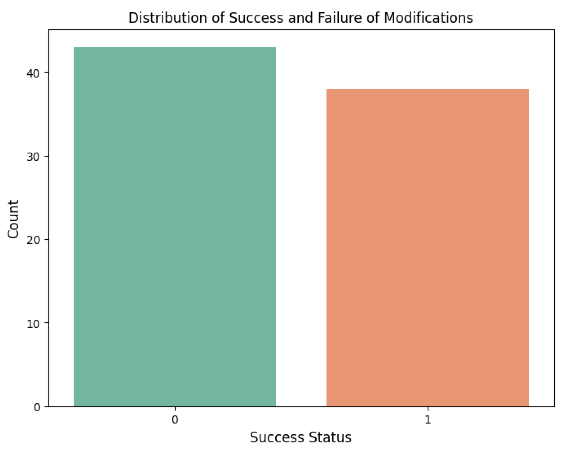
Figure 2. Distribution of Time Taken (in seconds) for Modification

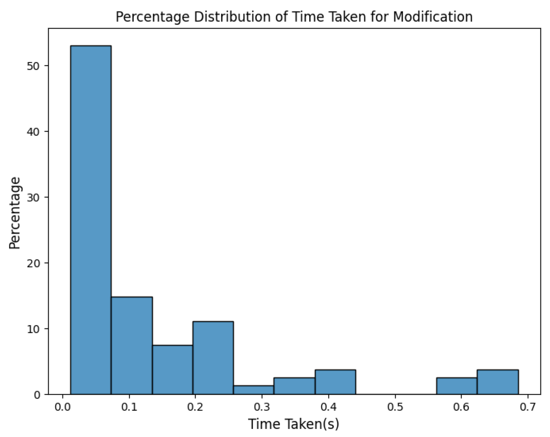
Figure 3. Comparison of Time Taken for Successful (1) vs Unsuccessful (0) Modifications

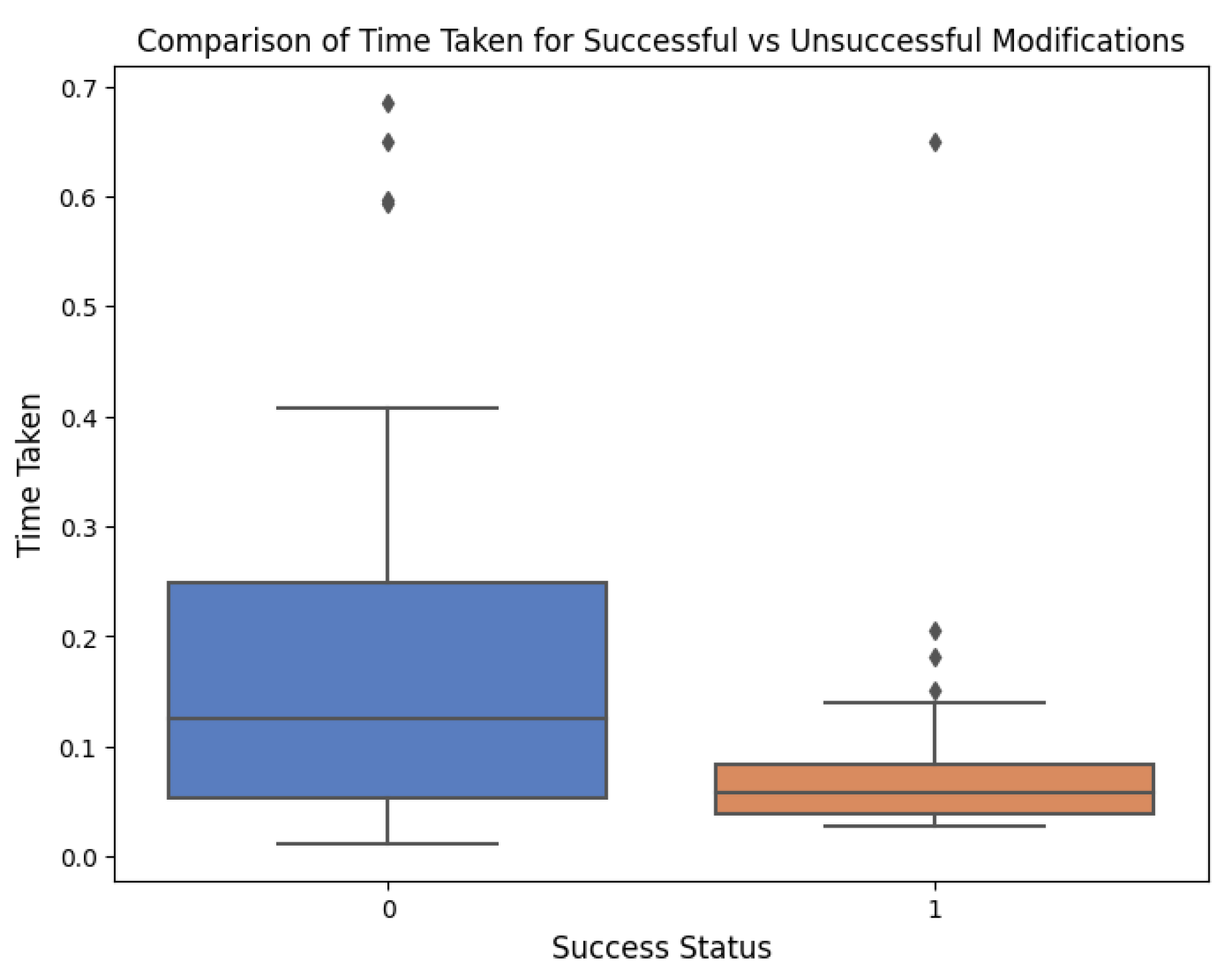
Table 1. Examples of high-precision explanations generated for tabular data from [2]

Adult Income
If	Predict
No capital gain or loss, never married	$\leq 50 K$
Country is US, married, work hours $> 45$	$> 50 K$
Lending a Loan
If	Predict
FICO score $\leq 649$	Bad Loan
$649 \leq$ FICO score $\leq 699$ and $$ 5, 400 \leq$ loan amount $\leq $ 10, 000$	Good Loan

Table 2. Actionable features in the HMEQ dataset including recourse actions

Feature	Description	Example recourse actions
LOAN	the amount of the loan request	increase (or reduce) loan request
MORTDUE	the amount due on the existing mortgage	pay down existing mortgage
VALUE	the current value of property	get updated property appraisal
DELINQ	the number of delinquent credit lines	pay off delinquent credit
NINQ	the number of recent credit inquiries	reduce credit applications
CLNO	the total number of credit lines	increase (or reduce) open credit lines
DEBTINC	the client’s current debt-to-income ratio	pay off some debt

Table 3. Ranges used for mapping continuous features into four discrete categories

Variable	Q1	Q2	Q3	Q4
LOAN	(1100.0, 23300.0)	(23300.0, 45500.0)	(45500.0, 67700.0)	(67700.0, 89900.0)
MORTDUE	(2063.0, 101434.75)	(101434.75, 200806.5)	(200806.5, 300178.25)	(300178.25, 399550.0)
VALUE	(8000.0, 219977.25)	(219977.25, 431954.5)	(431954.5, 643931.75)	(643931.75, 855909.0)
DELINQ	(0.0, 3.75)	(3.75, 7.5)	(7.5, 11.25)	(11.25, 15.0)
NINQ	(0.0, 4.25)	(4.25, 8.5)	(8.5, 12.75)	(12.75, 17.0)
CLNO	(0.0, 17.75)	(17.75, 35.5)	(35.5, 53.25)	(53.25, 71.0)
DEBTINC	(0.52, 51.22)	(51.22, 101.92)	(101.92, 152.62)	(152.62, 203.31)

Table 4. Performance metrics of Random Forest and XGBoost under different data split ratios

Model	Data Split Ratio	Accuracy	Precision	Recall	F1-score
Random Forest	80%-10%-10%	0.90	0.92	0.63	0.75
	70%-15%-15%	0.90	0.92	0.58	0.71
	60%-20%-20%	0.91	0.88	0.61	0.72
XGBoost	80%-10%-10%	0.90	0.90	0.61	0.73
	70%-15%-15%	0.89	0.88	0.57	0.69
	60%-20%-20%	0.91	0.85	0.62	0.72

Table 5. Parameters for Random Forest and XGBoost models

Model	Parameters
Random Forest	n_estimators=100, n_jobs=5, criterion=’log_loss’, max_features=’log2’
XGBoost	eval_metric=’logloss’, max_depth=6, subsample=0.8, colsample_bytree=0.8, n_estimators=100

Table 6. Performance metrics for different beam sizes and ignore indices conditions

Ignore indices	Beam Size	Success	Failure	Total Time (s)
TRUE	3	35	46	13.99
	5	37	44	10.87
	10	38	43	11.39
FALSE	3	55	26	213.78
	5	59	22	110.81
	10	59	22	151.1

Table 7. Mean time for Successful and Unsuccessful Modifications

Success Status	Mean Time (s)
Successful	0.08
Unsuccessful	0.19

Table 8. Variable changes and time taken for modification and evaluation

Changes (Variable: Original → Modified)	Time Taken (s)
DELINQ: (4.0 → 2.0)	0.063
LOAN: (1.0 → 2.0), NINQ: (4.0 → 2.0)	0.65
CLNO: (2.0 → 3.0)	0.06
MORTDUE: (1.0 → 0.0)	0.04
LOAN: (1.0 → 2.0), VALUE: (1.0 → 0.0)	0.15
NINQ: (4.0 → 0.0)	0.03
DELINQ: (3.0 → 0.0) , CLNO: (2.0 → 0.0)	0.21

Disclaimer/Publisher’s Note: The statements, opinions and data contained in all publications are solely those of the individual author(s) and contributor(s) and not of MDPI and/or the editor(s). MDPI and/or the editor(s) disclaim responsibility for any injury to people or property resulting from any ideas, methods, instructions or products referred to in the content.

© 2023 by the authors. Licensee MDPI, Basel, Switzerland. This article is an open access article distributed under the terms and conditions of the Creative Commons Attribution (CC BY) license (http://creativecommons.org/licenses/by/4.0/).

Copyright: This open access article is published under a Creative Commons CC BY 4.0 license, which permit the free download, distribution, and reuse, provided that the author and preprint are cited in any reuse.

Altmetrics

Downloads

130

Views

151

Comments

Subscription

Notify me about updates to this article or when a peer-reviewed version is published.

MDPI Initiatives

Important Links

Choose an area of interest and we will send you notifications of new preprints at your preferred frequency.

Disclaimer

Achievable Minimally Contrastive Counterfactual Explanations

Abstract

Keywords:

Subject:

1. Introduction

2. Related Work

3. Materials and Methods

3.1. Algorithm for Generating Achievable Counterfactuals

3.2. Procedure for Evaluating Counterfactuals

4. Experiments and Results

4.1. Dataset Selection and Preparation

4.2. Assessment of Classifier Performance

4.3. Setup for Machine Learning Models

4.4. Evaluation of the BFS_AMCC Approach

4.5. Evaluation of Impact of Beam Size

4.6. Examples of BFS_AMCC Modifications that Improve Predicted Outcomes

5. Discussion

6. Conclusions

Author Contributions

Funding

Data Availability Statement

Acknowledgments

Conflicts of Interest

Abbreviations

References

MDPI Initiatives

Important Links

Subscribe