A Richness Estimator Based on Integrated Data

Chun-Huo Chiu

doi:10.20944/preprints202307.0579.v1

Preprint

Article

A Richness Estimator Based on Integrated Data

This version is not peer-reviewed.

Chun-Huo Chiu^*

This version is not peer-reviewed.

Altmetrics

Downloads

Views

Comments

Submitted:

09 July 2023

Posted:

10 July 2023

You are already at the latest version

A peer-reviewed article of this preprint also exists.

Abstract

Species richness is a widely used measure for assessing the diversity of a particular area. However, observed richness often underestimates the true richness due to resource limitations, particularly in the small-sized sample or highly heterogeneous assemblage. Estimating species richness in a large-scale region typically involves an integrated data set consisting of subsamples collected independently from different subregions. However, the pooled sample of integrated data is no longer a random sample from the entire region, and the use of different sampling schemes results in variations in data formats. Consequently, employing a single sampling distribution to model the pooled sample becomes impractical, rendering existing richness estimators inadequate. This study theoretically explains the applicability of Chao's lower bound estimators in estimating species richness for large-scale areas using the pooled sample. Additionally, a new nonparametric estimator is introduced, which adjusts the bias of Chao's lower bound estimator by leveraging the Good-Turing frequency formula. This proposed estimator only utilizes the pooled sample's singleton, doubleton, and tripleton richness. Simulated data sets across various models are employed to demonstrate the statistical performance of the estimator, showcasing its ability to reduce bias and provide accurate 95% confidence intervals. Real data sets are also utilized to illustrate the practical application of the proposed approach.

Keywords:

Chao’s lower bound estimator; Good-Turing frequency formula; Integrated data; singleton; doubleton; tripleton

Subject:

Environmental and Earth Sciences - Ecology

1. Introduction

Species richness is the most commonly used quantitative diversity metric and is easily understood. The term "species" can be broadly defined to include biological species, software bugs, words in a book, genes, alleles, or other discrete entities, as reviewed in [1,2,3]. This article focuses on biological applications, specifically the number of detectable species within a given area. Ecological studies use two primary data formats to assess species diversity: individual-based abundance data and sample-based incidence data. Individual-based abundance data involve randomly sampling and identifying individual organisms to species. Sample-based incidence data involve randomly sampling a plot, quadrat, trap, transect, or net from the target region and recording the incidence of species appearing in the sampled unit.

However, producing an inventory species list in a target area is impossible due to resource or sampling limitations. In practice, a random sample from the target community, i.e., a small proportion of area size or community size in the target area, is typically used to assess species diversity; as such, the observed richness in the sampled sample always underestimates true richness. To address the negative bias of observed richness, dozens of estimators have been proposed for these two types of data and have led to considerable progress in various disciplines[1,2,4,5]. In ecological studies, the most widely used estimators are Chao’s lower bound estimators [6,7] and Jackknife-based estimators[8,9]. These estimators were derived without making assumptions about species detection rates. They are classified as nonparametric approaches and, as such, provide more robust estimates. In addition, these nonparametric estimators do not require all the information on observed species; only rare species (singletons and doubletons) are used in the sample to estimate undetected richness. These estimators could show expected robust statistical behavior only when the sampling unit (i.e. a individual in abundance data and a plot in incidence data) is indpendently or randomly sampled. However, due to resource constraints, a random sample is often only feasible in a limited area of a local region and not in a large-scale region.

In recent decades, monitoring species richness to reveal the impact of human activities on a large or global scale is an increasingly urgent task [10,11,12,13]. However, richness estimation of a large-scale region (or multiple communities) is still a statistical challenge for which no reliable estimator has been developed until now. In general, the collected data sets used to estimate the richness of a large-scale region usually consist of many samples that are separately sampled from the subregions by implementing different sampling schemes. Therefore, this integrated data set is composed of different kinds of data formats including individual-based abundance data and sample-based incidence data. However, the widely-used rigorous estimators in the literature have their limitations due to their underlying theoretical assumptions and are not equipped to analyze this type of integrated data.

In this article, I provide a theoretical interpretation of the applicability of Chao's lower bound estimator for estimating species richness based on a pooled sample of integrated data. Additionally, utilizing the Good-Turing frequency formula[14], I address the negative bias inherent in Chao's lower bound estimator and propose a bias-corrected alternative. The variance of the new estimator can be calculated through the asymptotic approach and its 95% confidence interval can be obtained through logarithmic transformation. To evaluate the efficacy of this proposed estimator, three commonly used ecological models and two real datasets are utilized in simulation studies and illustrative examples.

2. Materials and Methods

2.1. Sampling distribution model

Assume there are a total of

S

distinct species in the assemblage of interest. In ecological studies, individual-based abundance data and sample-based incidence data are the most commonly collected data types to assess richness diversity [15]. The sampling unit of individual-based abundance data is an individual randomly sampled and identified to species, and the sampling unit of sample-based incidence data is a plot, quadrat, trap, transect or net randomly sampled from the target subregion and only the incidence (presnece or absence) of species appearing in the selected plot is recorded.

For individual-based abundance data, assume

n

(a small fraction of assemblage size) individuals are randomly sampled and identified to species from the target region by sampling with replacement or sampling without replacement. Let

X_{i}

be the number of individuals of species i counted in the sample. The species frequency or species abundance

(X_{1}, X_{2}, \dots, X_{S})

could be assumed to follow a multinomial distribution with size n and probabilities

(p_{1}, p_{2}, \dots, p_{S})

and the species frequency

X_{i}

follows a binomial distribution with parameters

n

and

p_{i}

X_{i} ~ B i n o m i a l (n, p_{i}), i = 1, 2, \dots, S,

where

p_{i}

is the relative detection probability of species i. Let

f_{k} = \sum_{i = 1}^{S} I (X_{i} = k)

be the number of species that are observed exactly k times in the sample,

k = 1, 2, \dots, n

. Therefore,

f_{0}, f_{1}, f_{2}, f_{3}

are respectively the unseen richness, singleton richness, doubleton richness and tripleton richness in abundance sample.

For sample-based incidence data, assume

t

sampling units are randomly sampled from the target region and only the incidence (presence or absence) of species in the sampled unit is recorded. Let

Y_{i}

be the number of units in which species i is detected in the t sampled units. Then,

Y_{i}

could be assumed to follow a binomial distribution with size t and probability

π_{i}, i = 1, 2, \dots, S

Y_{i} ~ B i n o m i a l (t, π_{i}), i = 1, 2, \dots, S,

where

π_{i}

is the detection probability of species i, which depends on the abundance, body size and color of species i as well as the investigator’s capability. Let

Q_{k} = \sum_{i = 1}^{S} I (Y_{i} = k)

be the number of species that are detected in exactly k out of t sampling units,

k = 1, 2, \dots t .

Therefore,

Q_{0}, Q_{1}, Q_{2}, Q_{3}

are respectively the unseen richness, singleton richness, doubleton richness and tripleton richness in the incidence sample.

2.2. Richness estimation for one assemblage based on integrated data

Assuming that N samples are randomly collected from the assemblage through various sampling schemes, including individual-unit-based and sample-unit-based sampling methods, the integrated data comprises two formats (i.e., abundance data and incidence data), as commonly seen in ecological studies. To determine the richness of the assemblage, Chao1 and Chao2[6,7] derived without model assumption on species detection rates are the most commonly used estimators, which are briefly outlined below.

2.2.1. Chao’s lower bound estimators

Based on the Cauchy-Schwarz inequality and without making any assumptions on species detection rates, Chao proposed lower bound estimators for richness in 1984 and 1987. These estimators were designed for individual-based abundance data and sample-based incidence data, and are referred to as the Chao1 and Chao2 estimators, respectively. The Chao1 and Chao2 estimators are separately expressed as

C h a o 1 = S_{o b s} + \{\begin{matrix} \frac{f_{1}^{2}}{2 f_{2}} & i f f_{2} > 0 \\ \frac{f_{1}^{} (f_{1} - 1)}{2} & i f f_{2} = 0 \end{matrix},

(1)

C h a o 2 = S_{o b s} + \{\begin{matrix} \frac{t - 1}{t} \frac{Q_{1}^{2}}{2 Q_{2}} & i f Q_{2} > 0 \\ \frac{t - 1}{t} \frac{Q_{1}^{} (Q_{1} - 1)}{2} & i f Q_{2} = 0 \end{matrix},

(2)

Chao’s lower bound estimators only use the frequency counts of the two rarest species (i.e. the numbers of singleton and doubleton species) in the sample to estimate undetected richness.

On the basis of the Cauchy-Schwarz inequality theory, Chao’s lower bound estimators are unbiased when the detection rates of species are homogeneous (i.e.

p_{i} = \frac{1}{S}

in Eq.1 or

π_{i} = c

in Eq.2, for

i = 1, 2, \dots, S

). In addition, according to the concept of the Good-Turing frequency formula[14], Chao et al.[16,17] shew that Chao’s lower bound estimators are nearly unbiased estimators only when rare species have approximately homogenous detection probabilities (or rates). Therefore, the degree of heterogeneity of abundant species in the assemblage contains no information about the unbiasedness of Chao’s lower bound estimators. When the detection rate of rare species is highly heterogeneous or the sample size is not large enough, in contrast to other parametric estimators, Chao1 or Chao2 can provide a lower bound and robust richness estimate [2,18]. However, Chao1 and Chao2 were separately derived based on different sampling models for abundance data and incidence data. Importantly, it still has no theoretical evidence or proof that the existing estimators can be used to estimate species richness using a pooled sample of integrated data.

2.2.2. Extension of Chao’s lower bound estimators for integrated data

Many richness estimators proposed in the literature, whether they are parametric or non-parametric, are designed for randomly sampled data. This means that the detection rate of a species for each random trial, such as a selected individual or plot, is assumed to be identical. These estimators assume that the underlying assumptions of the binomial distribution are met

However, if N samples are collected using different sampling methods (e.g. sampling schemes, sampling efforts, plot sizes, or investigators) from the target region, the observed species count in the pooled sample no longer follows a binomial distribution. This violates the theoretical assumption of a random sample. This type of integrated data is often encountered in ecological studies where individual-based abundance data and sample-based incidence data are collected from the same target region. Although integrated data is widely used to estimate the richness of a large-scale or global region, no richness estimator has been rigorously designed to handle integrated data. In this section, I demonstrate theoretically that Chao's lower bound estimator can be modified to handle integrated data.

For individual-based abundance data, according to probability theory, when sample size

n

is sufficiently large and relative abundance (or detection probability)

p_{}

is sufficiently small, the species frequency (

X_{}

) follows a binomial distribution that converges to a Poisson distribution. It implies that the frequency (

X

) of rare species (i.e.

p_{}

is sufficiently small) in the sample could approximate a Poisson distribution with mean

n_{} p_{}

( i.e.

X_{} ~ p o i (n p_{})

) for species with low detection rate. This convergence feature also applies to sample-based incidence data. When the number of plots

t

is large and the detection rate

π_{}

tends to zero, the incidence count (

Y_{}

) of rare species in the sample could approximate a poison distribution with mean

t_{} π_{}

( i.e.

Y_{} ~ p o i (t π)

) for species with low detection rate.

Without loss of generality, two random samples are collected from the target region through different sampling schemes, namely individual-based sampling and plot-based sampling methods. These samples correspond to individual-based abundance data and sample-based incidence data, respectively. When the two sampled samples are pooled, the pooled species frequency

Z_{i} = X_{i} + Y_{i}

represents the count of species i in the pooled sample. Here,

Z_{i}

is no longer a random variable following a binomial distribution.

Based on the convergence principle between the binomial and Poisson distributions discussed earlier, we have, for species with low detection rates in the combined sampling scheme (i.e. small

p_{i}

and small

π_{i}

), the abundance (

Z_{i}

) in the pooled sample approximately follows a Poisson distribution with mean parameter

λ_{i} = n p_{i} + t π_{i}

. For simplicity, let denote this mean parameter as

{λ_{i} = m d}_{i}

, where

m

represents the unknown size of the pooled sample and

d_{i}

represents the detection rate of species i. Next, let

G_{k} = \sum_{i = 1}^{S} I (Z_{i} = k)

be the species frequency count, representing the number of species that are present exactly k times in the pooled sample. When k is small (e.g. k = 0, 1, 2 or 3) and the size of the pooled sample is sufficiently large,

G_{k}

is primarily contributed by the rare species, which approximately follow a Poisson distribution. Given a specific sampling scheme, all species in the region can be divided into a set of rare species denoted as

{s_{r a r e}}

and a set of abundant species denoted as

{s_{a b u n}}

. Based on the existing convergence theory between the binomial distribution and the Poisson distribution, we have the approximation of the expectation of

G_{k}

for small k,

E [G_{k}] = E [\sum_{i = 1}^{S} I (Z_{i} = k)] = \sum_{i \in \{S_{r a r e}\}} P (Z_{i} = k) + \sum_{i \in \{S_{a b u n}\}} P (Z_{i} = k)

Since when k is small, the probability that abundant species have a count of k tends to zero. Therefore,

\sum_{i \in \{S_{a b u n}\}} P (Z_{i} = k)

is roughly equal to 0. We have

E [G_{k}] \approx \sum_{i \in \{S_{r a r e}\}} P (Z_{i} = k) + 0 .

According to the convergence property between binomial and Poisson distribution for rare species, the following approximation is held:

E [G_{k}] \approx \sum_{i \in \{S_{r a r e}\}} P (Z_{i} = k) \approx \sum_{i \in \{S_{r a r e}\}} \frac{λ_{i}^{k}}{k!} e^{- λ_{i}} \approx \sum_{i = 1}^{S} \frac{λ_{i}^{k}}{k!} e^{- λ_{i}} .

Therefore, we can derive the following four approximation equations for the expectation of undetected richness, singleton richness, doubleton richness, and tripleton richness, which represent the number of rare species in the pooled sample.

E [G_{0}] = E [\sum_{i = 1}^{S} I (Z_{i} = 0)] = \sum_{i = 1}^{S} P (Z_{i} = 0) \approx \sum_{i = 1}^{S} e^{- λ_{i}}

(3.1)

E [G_{1}] = E [\sum_{i = 1}^{S} I (Z_{i} = 1)] = \sum_{i = 1}^{S} P (Z_{i} = 1) \approx \sum_{i = 1}^{S} {{λ_{i}}^{} e}^{- λ_{i}}

(3.2)

E [G_{2}] = E [\sum_{i = 1}^{S} I (Z_{i} = 2)] = \sum_{i = 1}^{S} P (Z_{i} = 2) \approx \sum_{i = 1}^{S} \frac{{λ_{i}}^{2}}{2} e^{- λ_{i}}

(3.3)

E [G_{3}] = E [\sum_{i = 1}^{S} I (Z_{i} = 3)] = \sum_{i = 1}^{S} P (Z_{i} = 3) \approx \sum_{i = 1}^{S} {\frac{{λ_{i}}^{3}}{6} e}^{- λ_{i}}

(3.4)

It is worth emphasizing once again that these approximations are valid only for lower species frequency counts in the sample, under the condition that sample sizes (

n

and

t

) are sufficiently large. In Appendix A, I provide evidence that the aforementioned approximate equations hold by demonstrating their validity through numerical simulations.

Based on the Cauchy-Schwarz inequality, we have the inequality

\sum_{i = 1}^{S} e^{- λ_{i}} \sum_{i = 1}^{S} {λ_{i}}^{2} e^{- λ_{i}} \geq {(\sum_{i = 1}^{S} {λ_{i}}^{} e^{- λ_{i}})}^{2},

(4)

According to Eqs. 3.1-3.2, Eq. 4 is equivalent to

E [G_{0}] E [2 G_{2}] \geq E {[G_{1}]}^{2}

. This inequality is also held when species detected mean abundance

λ_{i}

is assumed to be a random variable with probability density function

f (λ)

, expressed as

(S \int e^{- λ_{}} f (λ) d λ) (S \int λ^{2} e^{- λ_{}} f (λ) d λ) \geq {(S \int λ^{} e^{- λ_{}} f (λ) d λ)}^{2} .

Therefore, we have the lower bound estimator of undetected richness

{\hat{G}}_{0} = \frac{G_{1}^{2}}{2 G_{2}},

which uses the number of singletons and doubletons in the pooled sample to estimate undetected richness. Therefore, the proposed richness estimator could be interpreted as an extension of Chao1 or Chao2. It is denoted as Chao3, and the modified formula can be expressed as

C h a o 3 = S_{o b s} + \{\begin{matrix} \frac{G_{1}^{2}}{2 G_{2}} & i f G_{2} > 0 \\ \frac{G_{1} (G_{1} - 1)}{2} & i f G_{2} = 0 \end{matrix}

(5)

2.2.3. Adjusted Lower bound estimator of species richness for integrated data

According to the Cauchy-Schwarz inequality, we know Chao3 is a lower bound estimator. Based on the concept of the Good-Turing frequency formula, Chao3 will be severely negatively biased when the rare species have a high degree of heterogeneity. In this section, the negative bias of Chao3 can be corrected based on the concept of Good-Turing frequency formula[14]. The bias of Chao3 is approximately equal to

E [\frac{G_{1}^{2}}{2 G_{2}}] - E [G_{0}] \approx \frac{{(\sum_{i = 1}^{S} {m d_{i}}^{} e^{- m d_{i}})}^{2}}{2 \sum_{i = 1}^{S} \frac{{(m d_{i})}^{2}}{2} e^{- m d_{i}}} - \sum_{i = 1}^{S} e^{- m d_{i}} .

Let

d_{(r)} = \sum_{i = 1}^{S} d_{i} I (Z_{i} = r) / G_{r}

be the mean detection rate of species which are present r times in the pooled sample; it can be estimated using the modified Good-Turing frequency formula as

{\hat{d}}_{(r)} = \frac{(r + 1) G_{r + 1}}{{m G}_{r}} .

Using the modified Good-Turing frequency formula, we have the following approximate equations

E [G_{1}] \approx \sum_{i = 1}^{S} {m d_{i}}^{} e^{- m d_{i}} = \sum_{i = 1}^{S} \frac{2}{m d_{i}} E [I (Z_{i} = 2)] \approx \frac{2}{{m d}_{(2)}} E [G_{2}]

(6.1)

E [G_{0}] \approx \sum_{i = 1}^{S} {e^{- m d_{i}}}^{} = \sum_{i = 1}^{S} \frac{1}{m d_{i}} E [I (Z_{i} = 1)] \approx \frac{1}{{m d}_{(1)}} E [G_{1}]

(6.2)

According to Eqs. 6.1-6.2, the bias of

\frac{G_{1}^{2}}{2 G_{2}}

can be approximately derived as

B i a s_{C h a o 3} = E [\frac{G_{1}^{2}}{2 G_{2}}] - E [G_{0}] \approx (\frac{1}{{m d}_{(2)}} - \frac{1}{{m d}_{(1)}}) E [G_{1}]

Therefore, the bias of Chao3 can be estimated by replacing

d_{(1)}

and

d_{(2)}

with

{\hat{d}}_{(1)}

and

{\hat{d}}_{(2)}

, respectively. It is given as

{\hat{B i a s}}_{C h a o 3} = \frac{G_{1}^{2}}{2 G_{2}} (\frac{2 G_{2}^{2}}{3 G_{1} G_{3}} - 1)

Then, we have the bias-corrected estimator of Chao3, expressed as

C h a o 3_{A d j} = S_{o b s} + {\frac{G_{1}^{2}}{2 G_{2}} (2 - \frac{2 G_{2}^{2}}{3 G_{1} G_{3}})}^{-},

(7)

where

{(A)}^{-}

equals

A

A < 1

and 1 if

A \geq 1

. Here,

G_{3}

(or

G_{1})

is replaced by 1 as

G_{3} = 0

(or

G_{1} = 0

) to make Eq. 7 always well-defined. The mathematic form of the estimator shown in Eq. 7 is identical to the parametric estimator proposed by Chiu[18, 19] which was derived based on the Beta-Binomial mixture model for sample-based incidence data or based on the Gamma-Poisson mixture model for individual-based abundance data. The new estimator can also be proved to be a lower bound of richness under the incidence-based Beta-Binomial mixture model or the abundance-based Gamma-Poisson mixture model [19,20].

Since the Chao3_Adj estimator utilizes the first three rarest species in the sample to estimate undetected richness, it can be applied to integrated data consisting of multiple samples randomly collected from the target region without adhering to a specific sampling model or scheme. In order to aid readers, a table has been created in Appendix B, which outlines the equations and symbols used in the proposed estimators, along with their meanings, origins (with references), as well as their advantages and disadvantages.

2.3. Regional richness estimation based on integrated data

When the target region is divided into N subregions, species sampling data are collected independently and separately from each subregion. The sampling data can be collected by either an individual-unit-based sampling method or a sample-unit-based sampling method. Let

X_{i j}

represent the number of sampling units (such as the number of individuals in individual-based abundance data or the number of plots in sample-based incidence data) of species

i

in the sample

j

, which is collected from the

j t h

subregion. Here, i ranges from 1 to

S

for the

S

species, and j ranges from 1 to

N

for the

N

subregions

.

If the sample size (i.e. the total number of individuals in abundance data or the total number of plots in incidence data) is sufficiently large in each sample, the counts (

X_{i j}

) of species with low detection rates will approximate a Poisson distribution. Then, the total count of species i in the pooled sample, denoetd as

X_{i +} = \sum_{j = 1}^{N} X_{i j}

, will approximate a Poisson distribution when the detection rate of species i in each subregion is uniformly low.

Letting

G_{k} = \sum_{i = 1}^{S} I (X_{i +} = k)

be the number of species with a count of exactly k in the pooled sample. The approximate equations shown in Eqs. 3.1-3.4 are also applicable to the pooled sample of integrated data. Additionally, formulas for Chao3 and Chao3_Adj can be derived to estimate regional species richness based on the Good-Turing frequency formula, without making any specific model assumptions. Similarly, their variance estimators can be obtained using the asymptotic approach, and the 95% confidence interval (CI) of species richness can be derived by referring to the discussion surrounding Eq. 9.

According to the derivation, the proposed richness estimator possesses the following properties: (i) When the samples are individually and randomly collected from each subregion, the sampled samples can be directly combined to estimate undetected richness, regardless of whether the data format in each sample is identical or not. (ii) The estimation of undetected richness is solely based on the frequency counts of the rarest species in the pooled sample. (iii) When the detection rates of rare species are homogeneous (including the homogeneous model as a special case) or the sample size is sufficiently large, the proposed estimators are nearly unbiased.

2.4. Variance estimation

To derive the variance estimators for the discussed richness estimators, an asymptotic approach is employed. By defining

G_{2 +}

as the total frequency count of species with a count of at least 3 in the sample (i.e.,

G_{2 +} = \sum_{k \geq 3}^{} G_{k}

), the estimator

{\hat{S}}_{C h a o 3}

can be expressed as a function of

(G_{1}, G_{2}, G_{2 +})

. The estimator of

{\hat{S}}_{C h a o 3}

’s variance could be obtained by the asymptotic approach in which

(G_{0}, G_{1}, G_{2}, G_{2 +})

approximate a multinomial distribution with parameters

(S, \frac{E [G_{0}]}{S}, \frac{E [G_{1}]}{S}, \frac{E [G_{2}]}{S}, \frac{E [G_{2 +}]}{S})

. Additionally, let

G_{4 +}

be the total frequency count of species with a count of at least 4 in the sample (i.e.,

G_{4 +} = \sum_{k \geq 4}^{} G_{k}

), then Chao3_Adj becomes a function of

(G_{1}, G_{2}, G_{3}, G_{4 +})

. The estimator of

S_{A d j . C h a o 3}

's variance can also be obtained using the asymptotic approach, where

(G_{0}, G_{1}, G_{2}, G_{3}, G_{4 +})

approximately follow a multinomial distribution with parameters

(S, \frac{E [G_{0}]}{S}, \frac{E [G_{1}]}{S}, \frac{E [G_{2}]}{S}, \frac{E [G_{3}]}{S}, \frac{E [G_{4 +}]}{S})

The variance estimator of the Chao3 or Chao3_Adj can be derived by the delta method and is expressed as

{\hat{v a r} ({\hat{S}}_{}}_{}) \approx \sum_{i}^{} \sum_{j}^{} \frac{\partial {\hat{S}}_{}_{}}{\partial G_{i}} \frac{\partial {\hat{S}}_{}_{}_{}}{\partial G_{j}} \hat{c o v} (G_{i}, G_{j}),

(8)

where

\hat{c o v} (G, G_{j}) = \{\begin{matrix} G_{i} (1 - G_{i} / {\hat{S}}_{}_{}) & i f i = j \\ - G_{i} G_{j} / {\hat{S}}_{} & i f i \neq j \end{matrix}

To derive the 95% confidence interval (CI) of species richness and to ensure the lower bound of the 95% CI of species richness is larger than the observed richness, assume

{\hat{S}}_{} - S_{o b s}

follows a log-normal distribution [18,21]. Then the two-sided 95% CI of species richness is obtained as

[S_{o b s} + \frac{{\hat{S}}_{} - S_{o b s}}{R}, S_{o b s} + (\hat{S} - S_{o b s}) R],

(9)

where

R = e x p \{1.96 {[\log (1 + \frac{V a r ({\hat{S}}_{})}{{({\hat{S}}_{} - S_{o b s})}^{2}})]}^{\frac{1}{2}}\}

When samples are randomly collected, Chao3 consistently provides a lower bound estimate of species richness. Similarly, the Chao3_Adj also provides a lower bound estimate of species richness under the Gamma-Poisson model or the Beta-Binomial model [19,20]. Therefore, in cases where the community exhibits high heterogeneity or the sample size is small, these two estimators can offer lower bound estimates and more informative one-sided 95% confidence intervals (CIs) of species richness, shown as

[S_{o b s} + \frac{{\hat{S}}_{} - S_{o b s}}{R}, \infty],

where

R = e x p \{1.65 {[\log (1 + \frac{V a r ({\hat{S}}_{})}{{({\hat{S}}_{} - S_{o b s})}^{2}})]}^{\frac{1}{2}}\}

3. Results

3.1. Simulation study

A simulation study was conducted to examine the statistical behaviors of the new estimators. The study involved the use of three species abundance models to generate individual-based abundance data and three species detection models to generate sample-based incidence data. The number of species was kept constant at S = 600, and the simulated datasets were generated separately and independently using the following models.

3.1.1. For individual-based abundance sampling models:

The species detection probabilities (or species relative abundance)

(p_{1}, p_{2}, \dots, p_{S}) = ({c a}_{1}, {c a}_{2}, \dots, {c a}_{S})

in each model are provided below, where c is a normalizing constant such that

\sum_{i = 1}^{S} p_{i} = 1

. The coefficient of variation (CV) of

(p_{1}, p_{2}, \dots, p_{S})

is also presented to indicate the degree of heterogeneity of

(p_{1}, p_{2}, \dots, p_{S})

a.: Abundance model 1, random uniform model (CV = 0.53): with $p_{i} = c a_{i}, i = 1, 2, \dots, S$ , where $(a_{1}, a_{2}, \dots, a_{S})$ is a random sample from a uniform distribution.
b.: Abundance model 2, broken-stick model (CV = 0.97): with $p_{i} = c a_{i}, i = 1, 2, \dots, S$ , where $(a_{1}, a_{2}, \dots, a_{S})$ is a random sample from an exponential distribution with parameter 1. This model is commonly used in the literature and is equivalent to the Dirichlet distribution.
c.: Abundance model 3, log-normal model (CV = 1.56): with $p_{i} = c a_{i}, i = 1, 2, \dots, S$ , where $(a_{1}, a_{2}, \dots, a_{S})$ is a random sample from a log-normal distribution with parameters 0 and 1.

3.1.2. For sample-based incidence sampling models

The species detection probabilities

(π_{1}, π_{2}, \dots, π_{S}) = ({c a}_{1}, {c a}_{2}, \dots, {c a}_{S})

in each model were determined, where c is a rescaling constant such that the maximum detection probability is a fixed at a constant value. The coefficient of variation (CV) of

(π_{1}, π_{2}, \dots, π_{S})

is also calculated to indicate the degree of heterogeneity of

(π_{1}, π_{2}, \dots, π_{S}) .

d: Incidence model 1: the random uniform model (CV = 0.57): where $π_{i} = c a_{i}, i = 1, 2, \dots, S$ , and $(a_{1}, a_{2}, \dots, a_{S})$ is a random sample from a uniform distribution

with parameters (0, 1), and scale c is used to control the maximum of $π_{i}$ .
e: Incidence model 2: the broken stick model (CV = 0.99): where $π_{i} = c a_{i}, i = 1, 2, \dots, S$ , and $(a_{1}, a_{2}, \dots, a_{S})$ is a random sample from an exponential distribution with parameter 1, and scale c is used to control the maximum of $π_{i}$ . This model is commonly used in the literature and equivalent to the Dirichlet distribution.
f: Incidence model 3: the log-normal model (CV = 1.23): where $π_{i} = c a_{i}, i = 1,2, \dots, S$ , and $(a_{1}, a_{2}, \dots, a_{S})$ is a random sample from a log-normal distribution, and scale c is used to control the maximum of $π_{i}$ .

The coefficient of variation (CV) in these six models ranged from 0 to 1.56, encompassing a wide range of values that encompass most practical cases in real-world applications.

In the simulation study, different sample sizes are considered to represent varying levels of sampling effort. For each simulation scenario, 1000 simulated datasets are generated. The estimates and their corresponding estimated standard errors (SE) are averaged across the 1000 simulated datasets to obtain the mean estimate and mean estimated SE. The sample SE and root-mean-square error (RMSE) are calculated based on the 1000 estimates to determine the sample SE and sample RMSE. The percentage of 95% confidence intervals (CIs) that cover the true value and the average observed richness are also calculated. All the simulation results are presented in Table 1 and Table 2. For simplicity, the average estimates of the discussed estimators are plotted in Figure 1 and Figure 2 to illustrate their statistical behavior as a function of sampling effort.

3.2. Simulation results for richness estimation of one assemblage (a local region)

In this case, the integrated dataset consists of three random samples that are independently collected from the same assemblage. Each sample is simulated separately based on one of the three discussed abundance/incidence models, representing different sampling situations or methods. Different sample sizes are considered to indicate varying levels of sampling efforts, ranging from n = 200 to 600 with an increment of 50 for abundance data and t = 10 to 50 with an increment of 5 for incidence data.

Four different scenarios are examined, including:

Three abundance models: random uniform, broken-stick, and log-normal.
Two abundance models: random uniform and broken-stick, along with one incidence model: log-normal.
One abundance model: random uniform, along with two incidence models: broken-stick and log-normal.
Three incidence models: random uniform, broken-stick, and log-normal.

The simulation results for these four scenarios are presented separately in Figure 1a–d and Table 1.

3.3. Simulation results for richness estimation of multiple assemblages (a large-scale region)

To evaluate the statistical behavior of the discussed estimators for regional richness estimation based on integrated data, the target region is divided into three subregions. The integrated data consists of three samples that are collected separately from each subregion. It is assumed that the target region comprises S = 600 species, with each subregion having 300 species. There are varying numbers of shared species and unique species in each subregion.

Different sample sizes are considered to represent different sampling efforts, ranging from n = 400 to 4000 with an increment of 450 for abundance data, and t = 10 to 50 with an increment of 5 for incidence data. Four different scenarios are examined, including:

Three abundance models: random uniform, broken-stick, and log-normal.
Two abundance models: random uniform and broken-stick, along with one incidence model: log-normal.
One abundance model: random uniform, along with two incidence models: broken-stick and log-normal.
Three incidence models: random uniform, broken-stick, and log-normal.

The simulation results for these four scenarios are presented separately in Figure 2a-d and Table 2.

Undoubtedly, for a fixed sample size, a superior species richness estimator should exhibit lower bias and variance (i.e., low RMSE). Additionally, the coverage rate of its associated 95% confidence interval should be close to 0.95. As the sample size increases, the estimator should demonstrate the following essential behaviors: its bias, accuracy (as measured by RMSE), and the coverage rate of its confidence interval should generally improve, eventually converging to the true species richness when the sample size is sufficiently large. Based on these criteria, the following findings can be concluded from the simulation results:

In all simulation scenarios presented in Table 1 and Table 2 and Figure 1 and Figure 2, both Chao3 and the proposed adjusted Chao3 (Chao3_Adj) consistently provide robust lower bound estimates in all hypothetical models, and they tend to approach the true richness as the sample size increases.
Both Chao3 and Chao3_Adj exhibit the essential statistical behaviors: their bias and RMSE decrease, resulting in more accurate 95% confidence intervals as the sample size increases (Table 1 and Table 2).
The estimators of the discussed estimators' variance, derived using the asymptotic approach, perform well across all simulation scenarios (Table 1 and Table 2).
Compared to Chao3, the adjusted estimator (Chao3_Adj) exhibits lower bias, larger standard errors, and more accurate 95% confidence intervals for the true richness in all simulation scenarios (Table 1 and Table 2).
When samples are directly collected from the entire region (Table 1), Chao3_Adj has higher RMSEs compared to Chao3. However, when samples are separately collected from subregions within the target region (Table 2), Chao3_Adj demonstrates lower RMSEs.

These findings collectively demonstrate the favorable performance of the proposed adjusted Chao3 estimator (Chao3_Adj) in terms of bias, standard error, and accuracy of the 95% confidence interval, particularly when samples are collected from subregions within the target region.

3.4. Using data sets as true assemblages

I utilized two biological survey datasets representing true assemblages and generated separate datasets from these two assemblages. In each dataset, the observed species relative abundance was considered as the true species relative abundance or detection probability. A sample of size n (or t) was then generated through sampling with replacement to create the sampling dataset. Different sample sizes were considered to indicate varying levels of sampling efforts.

The average estimate and other relevant statistics obtained using the 1,000 generated datasets, as a function of sample size, are depicted in Figure 3 and Figure 4 and supplemental Table C1 and Table C2 (refer to Appendix C for detailed information). These evaluations aimed to assess the statistical behaviors of the discussed richness estimators across four different sampling scenarios: three abundance data, two abundance data and one incidence data, one abundance data and two incidence data, and three incidence data.

3.4.1. Moth species data

Moth species data were collected in the Golfo Dulce region of the Costa Rican rainforest from July to October 2014 [22]. The target region was divided into three types of forest: creek forest, slope forest, and ridge forest. Light traps were set up at 18 sites, with six replicates within each forest type. Further details can be found in [22].

Table 3 presents a summary of the data, including the sample size, observed richness, and the first five species frequency counts for each forest type. In the pooled sample, a total of 421 species were recorded, with 115, 285, and 356 species observed in the creek, slope, and ridge forests, respectively. In this case, the survey data sets are considered as the true assemblages. The proportion of species in the sample is assumed to represent the species' relative abundance for generating individual-based abundance data, while the ratio between species abundance and the maximum abundance is considered as the species' detection probability for generating sample-based incidence data. Consequently, each type of forest has its corresponding abundance model and incidence model. Four different scenarios are examined, including:

Three abundance models: creek, slope, and ridge.
Two abundance models: creek and slope, along with one incidence model: ridge.
One abundance model: creek, along with two incidence models: slope and ridge.
Three incidence models: creek, slope, and ridge.

The simulation results for each scenario are depicted separately in Figure 3a-3d and Supplementary Table C1 (Appendix C).

3.4.2. xylobiont beetle species data

The second real dataset comprises xylobiont beetle species data collected from the Leipzig floodplain forest in 2016 [23]. The beetle species data were collected separately from three dominant tree species: Quercus robur (QR), Tilia cordata (TC), and Fraxinus excelsior (FE) in the Leipzig floodplain forest area. Table 3 provides information on the sample size, observed richness, and the first three species frequency counts for each tree species. In total, 307 beetle species were observed, with 174, 198, and 184 species recorded in QR, TC, and FE tree species, respectively.

In this case, the survey data sets are treated as the true assemblages, and the species abundance/incidence model is constructed using the same method discussed earlier for each tree species. Four different scenarios are considered, including:

Three abundance models: QR, TC, and FE.
Two abundance models: QR and TC, along with one incidence model: FE.
One abundance model: QR, along with two incidence models: TC and FE.
Three incidence models: QR, TC, and FE.

The simulation results for each scenario are presented separately in Figure 4a-d and Supplementary Table C2 (Appendix C).

The results from the analysis, as depicted in Figure 3 and Figure 4 and Supplemental Tables in Appendix C, demonstrate that both Chao3 and the adjusted Chao3 (Chao3_Adj) effectively reduce the underestimation of observed richness. From a theoretical standpoint and considering the results of the simulation study, it is expected that Chao3_Adj exhibits lower bias compared to Chao3, particularly when there is high heterogeneity as indicated by a high coefficient of variation (CV). Furthermore, the supplemental Table C1 and Table C2 in Appendix C confirm that Chao3_Adj has lower bias, higher standard error, and lower root-mean-square error (RMSE). The higher estimated standard error of Chao3_Adj compared to Chao3 suggests that the former estimator may provide a more accurate 95% confidence interval for true richness. This observation aligns with the findings of the simulation study presented in Table 1 and Table 2.

Overall, the results support the notion that Chao3_Adj has less bias and performs better in terms of standard error and RMSE, indicating its potential to provide more accurate estimates and confidence intervals for true richness, particularly in scenarios with higher heterogeneity.

4. Discussion and Conclusion

Estimating species richness for a large-scale region or multiple assemblages poses a statistical challenge due to the difficulty of obtaining a random sample from the entire region. Typically, data collected for assessing species richness in such cases consist of multiple samples that are individually sampled from each assemblage or subregion. Additionally, these samples may employ different sampling schemes or strategies. As a result, the pooled sample cannot be considered a random sample from the entire region, even though each individual sample is randomly collected from its respective subregion or assemblage. Consequently, the pooled sample cannot be modeled using a traditional sampling distribution model.

However, certain richness estimators that rely only on the frequency counts of rare species in the sample have been theoretically demonstrated to be applicable to the pooled sample, as long as the samples are randomly collected and the sample size is not excessively small. In this context, the detection probability of a species may vary across the samples, and the data format (individual-based abundance data or sample-based incidence data) can differ among the samples.

In this research, Chao's lower bound estimator (Chao3) and its bias-corrected estimator (Chao3_Adj) are theoretically proven to be suitable for estimating richness in multiple assemblages. Chao3 is derived using the Cauchy-Schwarz inequality, while the adjusted estimator (Chao3_Adj) corrects the bias of Chao3 based on the Good-Turing frequency formula[14]. Simulation results demonstrate that both Chao3 and Chao3_Adj can be used to estimate regional richness based on the pooled sample from integrated data, aligning with the theoretical findings. These estimators provide lower bound estimates in all hypothetical models and tend to converge to the true richness as the sample size increases. Notably, when the sample size is small or the community exhibits high heterogeneity, Chao3_Adj outperforms Chao3 with lower bias, lower root-mean-square error (RMSE), higher standard error (s.e.), and a more accurate 95% confidence interval (CI) for true richness.

Data Availability Statement

All R codes used in this paper are archived on Zenodo: https://doi.org/10.5281/zenodo.8118860. The moth species dataset used in this paper is archived on the website: https://doi.org/10.5061/dryad.783p8m2. The xylobiont beetle species dataset used in this paper is archived on the website: https://doi.org/10.5061/dryad.d7wm37q0g.

Conflicts of Interest

The authors declare no conflict of interest.

Appendix A: Numerical study to show that the expectation of species count of rare frequency in the pooled sample is approximately identical to the probability sum of Poisson distribution.

Assuming there are

S

(=400) species contained in the target region. When abundance data and incidence data are collected from same region, assuming that species abundance (

X_{i}

) follows a binomial distribution with size

n

and probability

p_{i}

(i.e.,

X_{i} ~ B i n o m i a l (n, p_{i})

), where

\sum_{i = 1}^{S} p_{i} = 1

and species incidence count (

Y_{i}

) follows a binomial distribution with size

t

and probability

π_{i}

(i.e.

Y_{i} ~ B i n o m i a l (t, π_{i})

), where

π_{i} \in (0, 1)

. Let the species frequency in the pooled sample as

Z_{i} = X_{i} + Y_{i}

, then

G_{k} = \sum_{i = 1}^{S} I (Z_{i} = k)

is the count of species frequency in the pooled sample.

Here, I implement a simulation study to show the following equation (Eq.A1) is approximately hold when sample size (n) and (t) is large and

k

is small (i.e.

k = 0, 1, 2, 3

E [G_{k}] = \sum_{i = 1}^{S} P (Z_{i} = k) \approx \sum_{i = 1}^{S} \frac{λ_{i}^{k}}{k!} e^{- λ_{i}}, w h e r e λ_{i} = n p_{i} + t π_{i}

(A1)

a.: For individual-based abundance sampling model, the species detection probabilities (or species relative abundance) $p_{i} = c a_{i} a n d a_{i} ~ U (0, 1), i = 1, \dots, S$ , where $c$ is a normalizing constant such that $\sum_{i = 1}^{S} p_{i} = 1$ .
b.: For sample-based incidence model, The species detection probabilities $π_{i} ~ U (0.05, 0.2), i = 1, 2, \dots, 50 a n d π_{i} ~ U (0.8,1), i = 51, 52, \dots, 100$ .

In the simulation study, different sample sizes are considered to indicate different sampling efforts. For each simulation scenario, 1000 simulated data sets are generated, then

G_{k}

is averaged over the 1,000 simulated data sets to estimate

E [G_{k}]

. The table below show that the equation (Eq.A1) could be roughly hold for

k = 0, 1, 2, 3

when sample size (n and t) is large enough.

Table A1. the expectation the count of the first 5 rare species frequencies.

Sample size		$k = 0$	$k = 1$	$k = 2$	$k = 3$	$k = 4$	$k = 5$
$n = 100, t = 10$	$\sum_{i = 1}^{S} \frac{λ_{i}^{k}}{k!} e^{- λ_{i}}$	59.4	65.1	43	23.4	14.3	13.6
$n = 100, t = 10$	$E [G_{k}]$	55.6	66.9	44.8	22	8	3.2
$n = 200, t = 20$	$\sum_{i = 1}^{S} \frac{λ_{i}^{k}}{k!} e^{- λ_{i}}$	21.9	39.9	42.8	35.8	25.7	16.3
$n = 200, t = 20$	$E [G_{k}]$	20.2	39.2	43.3	37.4	27.1	17
$n = 300, t = 30$	$\sum_{i = 1}^{S} \frac{λ_{i}^{k}}{k!} e^{- λ_{i}}$	9.4	22.4	30.5	32	29.3	24.4
$n = 300, t = 30$	$E [G_{k}]$	8.5	21.5	30	32.5	29.9	25.7
$n = 400, t = 40$	$\sum_{i = 1}^{S} \frac{λ_{i}^{k}}{k!} e^{- λ_{i}}$	4.4	12.8	20.5	24.7	25.6	24.3
$n = 400, t = 40$	$E [G_{k}]$	4	12	20	24.5	25.4	24.8
$n = 500, t = 50$	$\sum_{i = 1}^{S} \frac{λ_{i}^{k}}{k!} e^{- λ_{i}}$	2.2	7.4	13.7	18.4	20.7	21.2
$n = 500, t = 50$	$E [G_{k}]$	1.9	6.9	13.1	18.1	20.6	21.2

The simulation results show that the expectations of first three frequency counts (i.e.

G_{0}, G_{1}, G_{2}, G_{3}

) are roughly identical to the probability sum of Poisson distribution with mean

λ_{i} = n p_{i} + t π_{i}, i = 1, 2, \dots, S .

Appendix B: The summary of the statistical properties of the richness estimators discussed in the text.

Available data and Notation	Richness estimator	Pluses and minuses
Individual-based abundance data: sampling unit is an individual randomly selected from target assemblage and identified to species S_obs: the observed richness. f₁: the singleton richness in the sample f₂: the doubleton richness in the sample . f₃: the tripleton richness in the sample	Chao1[6] $S_{o b s} + \{\begin{matrix} \frac{f_{1}^{2}}{2 f_{2}} & i f f_{2} > 0 \\ \frac{f_{1}^{} (f_{1} - 1)}{2} & i f f_{2} = 0 \end{matrix}$	1. A lower bound estimator of richness for all species composition models. 2. A nearly unbiased estimator when rare species are homogeneous 3. Has severely negative bias when community is highly heterogeneous.
	Chao1_Adj[19] $S_{o b s} + \frac{f_{1}^{2}}{2 f_{2}} {(2 - \frac{2 f_{2}^{2}}{3 f_{1} f_{3}})}^{-}$	1. A lower bound estimator of richness for Gamma-Poisson models. 2. Compare to $C h a o 1$ , $C h a o 1_{a d j}$ has less bias, higher variance, lower RMSE, and has more accurate coverage rate of 95% confidence interval.
Sample-based incidence data: sampling unit is a quadrat or plot and only the incidence of species appearing in the selected plot is recorded . S_obs: the observed richness. Q₁: the singleton richness in the sample. Q₂: the doubleton richness in the sample. Q₃: the tripleton richness in the sample/ t: the number of selected plot.	Chao2[7] $S_{o b s} + \{\begin{matrix} \frac{t - 1}{t} \frac{Q_{1}^{2}}{2 Q_{2}} & i f Q_{2} > 0 \\ \frac{t - 1}{t} \frac{Q_{1}^{} (Q_{1} - 1)}{2} & i f Q_{2} = 0 \end{matrix}$	1. A lower bound estimator of richness for all species composition model. 2. A nearly unbiased estimator when rare species are homogeneous 3. Has severely negative bias when community is highly heterogeneous.
	Chao2_Adj[20] $S_{o b s} + \frac{t - 1}{t} \frac{Q_{1}^{2}}{2 Q_{2}} {(2 - \frac{2 Q_{2}^{2}}{3 Q_{1} Q_{3}})}^{-}$	1. A lower bound estimator of richness for Beta-Binomial models. 2. Compare to $C h a o 2$ , $C h a o 2_{a d j}$ has less bias, higher variance, lower RMSE, and has more accurate coverage rate of 95% confidence interval.
Pooled sample of integrated data: directly pool the individual-based abundance data and sample-based incidence data as a new sample S_obs: the observed richness. G₁: the singleton richness in pooled sample. G₂: the doubleton richness in the pooled sample. G₃: the tripleton richness in the pooled sample.	Chao3 (New proposed) $S_{o b s} + \{\begin{matrix} \frac{G_{1}^{2}}{2 G_{2}} & i f G_{2} > 0 \\ \frac{G_{1} (G_{1} - 1)}{2} & i f G_{2} = 0 \end{matrix}$	1. Chao3 is available for pooled sample of integrated data. 2. A lower bound estimator of richness when sample size is large enough. 3. Has severely negative bias when community is highly heterogeneous.
	Chao3_Adj(New proposed) $S_{o b s} + \frac{G_{1}^{2}}{2 G_{2}} {(2 - \frac{2 G_{2}^{2}}{3 G_{1} G_{3}})}^{-}$	1. Compare to $C h a o 3$ , $C h a o 3_{a d j}$ has less bias, higher variance and lower RMSE. 2. Has more accurate coverage rate of 95% confidence interval.

Appendix C: Supplementary tables (Table A1 and Table A2)

Table C2. The statistical behavior of Chao3 and Chao3_Adj were analyzed in four scenarios to estimate the number of the moth species (richness=421) [22].

Size (Observed richness)	Estimator	Average Estimate	Bias	Sample SE	Average Estimated SE	Sample RMSE	95% CI Coverage Rate
Scenerio1
100,300,400 (200.0)	Chao3	301.6	-119.4	30.4	29.4	123.2	0.158
100,300,400 (200.0)	Chao3_Adj	350.7	-70.3^†	57.8	56.8	91^†	0.85^†
300,900,1000 (288.2)	Chao3	367.6	-53.4	22.1	22.4	57.8	0.49
300,900,1000 (288.2)	Chao3_Adj	399.1	-21.9^†	39.6	41.7	45.2^†	0.926^†
500,1500,1600 (328.2)	Chao3	391.9	-29.1	19.8	18.7	35.2^†	0.754
500,1500,1600 (328.2)	Chao3_Adj	416.4	-4.6^†	36.1	34.1	36.3	0.943^†
Scenerio2
100,300,10 (201.2)	Chao3	303.7	-117.3	30.1	29.5	121.1	0.18
100,300,10 (201.2)	Chao3_Adj	353.4	-67.6^†	58.3	56.9	89.2^†	0.846^†
300,900,30 (297.3)	Chao3	333	-88	30.5	27.2	93.1	0.294
300,900,30 (297.3)	Chao3_Adj	377.2	-43.8^†	57.9	51.9	72.6^†	0.891^†
500,1500,50 (338.4)	Chao3	351.8	-69.2	26	25.1	73.9	0.408
500,1500,50 (338.4)	Chao3_Adj	389	-32^†	49	47.2	58.5^†	0.931^†
Scenerio3
100,10,10 (200)	Chao3	310.2	-110.8	29.4	28.8	114.7	0.186
100,10,10 (200)	Chao3_Adj	357.1	-63.9^†	56.3	54.8	85.1^†	0.846^†
300,30,30 (288.2)	Chao3	339.2	-81.8	28.6	26.5	86.7	0.32
300,30,30 (288.2)	Chao3_Adj	380	-41^†	54.7	49.6	68.3^†	0.882^†
500,50,50 (328.2)	Chao3	357.2	-63.8	24.5	24.3	68.3	0.4
500,50,50 (328.2)	Chao3_Adj	393.7	-27.3^†	46.5	45.9	53.9^†	0.942^†
Scenerio4
10,10,10 (221.1)	Chao3	313.3	-107.7	28.7	26.7	111.4	0.168
10,10,10 (221.1)	Chao3_Adj	356.3	-64.7^†	54.6	50.9	84.6^†	0.842^†
30,30,30 (311.1)	Chao3	341.3	-79.7	25.4	25	83.7	0.286
30,30,30 (311.1)	Chao3_Adj	379.5	-41.5^†	47.6	47	63.1^†	0.911^†
50,50,50 (348.0)	Chao3	359.3	-61.7	23.6	23.2	66	0.428
50,50,50 (348.0)	Chao3_Adj	393.7	-27.3^†	44.4	43.3	52.1^†	0.941^†

Note: data in Scenerio1, Scenerio2, Scemerio3 and Scenerio4 are separately composed by three abundance data, two abundance data and one incidence data, one abundance data and two incidence data, and three incidence data.

†

denotes the least bias, lowest RMSE, and closest to 95% coverage. Abbreviations: SE, standard error; RMSE, root mean square error; CI, confidence interval;

Table C3. The statistical behavior of Chao3 and Chao3_Adj were analyzed in four scenarios to estimate the number of the beetle species (richness=207) in Leipzig floodplain forest[23].

Size (Observed richness)	Estimator	Average Estimate	Bias	Sample SE	Average Estimated SE	Sample RMSE	95% CI Coverage Rate
Scenerio1
200,200,200 (132.2)	Chao3	212.3	-94.7	29.9	29.1	99.3	0.321
200,200,200 (132.2)	Chao3_Adj	253.7	-53.3^†	59	56.2	79.5^†	0.856^†
600,600,600 (196.4)	Chao3	233.7	-73.3	28.4	27.4	78.6	0.428
600,600,600 (196.4)	Chao3_Adj	271.6	-35.4^†	55.4	52.5	65.8^†	0.912^†
1000,1000,1000 (228.1)	Chao3	250	-57	28.3	26.5	63.6	0.561
1000,1000,1000 (228.1)	Chao3_Adj	287.6	-19.4^†	54.4	50.5	57.7^†	0.928^†
Scenerio2
200,200,10 (115.7)	Chao3	199.1	-107.9	34.6	31.8	113.3	0.287
200,200,10 (115.7)	Chao3_Adj	245.9	-61.1^†	69.2	62.3	92.3^†	0.841^†
600,600,30 (181.3)	Chao3	221.3	-85.7	30.3	29.5	91	0.386
600,600,30 (181.3)	Chao3_Adj	263.1	-43.9^†	59.7	56.9	74.1^†	0.892^†
1000,1000,50 (215.8)	Chao3	238.3	-68.7	30.3	28.3	75.1	0.497
1000,1000,50 (215.8)	Chao3_Adj	278.8	-28.2^†	59.7	54	66^†	0.912^†
Scenerio3
200,10,10 (127.5)	Chao3	209.3	-97.7	30.4	30	102.3	0.334
200,10,10 (127.5)	Chao3_Adj	252.2	-54.8^†	59.4	58.5	80.8^†	0.855^†
600,30,30 (195.4)	Chao3	232	-75	29.1	27.8	80.5	0.43
600,30,30 (195.4)	Chao3_Adj	269.9	-37.1^†	57.1	52.9	68.1^†	0.885^†
1000,50,50 (227.8)	Chao3	245.5	-61.5	26.4	25.3	66.9	0.504
1000,50,50 (227.8)	Chao3_Adj	278.4	-28.6^†	50.4	47.7	57.9^†	0.929^†
Scenerio4
10,10,10 (141.1)	Chao3	228.5	-78.5	33.2	31	85.2	0.453
10,10,10 (141.1)	Chao3_Adj	274.3	-32.7^†	66.1	60.3	73.7^†	0.882^†
30,30,30 (213.0)	Chao3	251.5	-55.5	27.9	28.5	62.2	0.613
30,30,30 (213.0)	Chao3_Adj	291.2	-15.8^†	55.1	54.3	57.3^†	0.916^†
50,50,50 (246.2)	Chao3	264.4	-42.6	27.8	25.6	50.8^†	0.685
50,50,50 (246.2)	Chao3_Adj	297.5	-9.5^†	52.7	47.7	53.6	0.922^†

†

denotes the least bias, lowest RMSE, and closest to 95% coverage. Abbreviations: SE, standard error; RMSE, root mean square error; CI, confidence interval;.

References

Bunge, J.; Fitzpatrick, M. Estimating the number of species: A review. J. Am. Stat. Assoc. 1993, 88, 364–373. [Google Scholar]
Colwell, R. K.; Coddington, J. A. Estimating terrestrial biodiversity through extrapolation. Philos. Trans. R. Soc. Lond. B Biol. Sci. 1994, 345, 101–118. [Google Scholar] [CrossRef]
Chao, A.; Chiu, C.-H. Species richness: estimation and comparison. Wiley StatsRef: statistics reference online 2016, 1, 26. [Google Scholar]
Wilson, R. M. a. C. M. F. M. Capture-recapture estimation with samples of size one using frequency data. Biometrika 1992, 79, 543–553. [Google Scholar]
Chao, A., Species estimation and applications. In Encyclopedia of statistical sciences, Balakrishnan, N.; Read, C. B.; Vidakovic, B., Eds. Wiley: New York, 2005; pp 7907-7916.
Chao, A. Nonparametric estimation of the number of classes in a population. Scand. J. Stat. 1984, 11 265-270.
Chao, A. Estimating the population size for capture-recapture data with unequal catchability. Biometrics 1987, 43, 783–791. [Google Scholar] [CrossRef]
Burnham, K. P.; Overton, W. S. Estimation of the size of a closed population when capture probabilities vary among animals. Biometrika 1978, 65, 625–633. [Google Scholar]
Burnham, K. P.; Overton, W. S. Robust estimation of population size when capture probabilities vary among animals. Ecology 1979, 60, 927–936. [Google Scholar] [CrossRef]
Bellard, C.; Bertelsmeier, C.; Leadley, P.; Thuiller, W.; Courchamp, F. Impacts of climate change on the future of biodiversity. Ecol. Lett. 2012, 15(4), 365–377. [Google Scholar] [CrossRef]
Cardinale, B. J.; Duffy, J. E.; Gonzalez, A.; Hooper, D. U.; Perrings, C.; Venail, P.; Narwani, A.; Mace, G. M.; Tilman, D.; Wardle, D. A. Biodiversity loss and its impact on humanity. Nature 2012, 486(7401), 59–67. [Google Scholar]
Cavicchioli, R.; Ripple, W. J.; Timmis, K. N.; Azam, F.; Bakken, L. R.; Baylis, M.; Behrenfeld, M. J.; Boetius, A.; Boyd, P. W.; Classen, A. T. Scientists’ warning to humanity: microorganisms and climate change. Nat. Rev. Microbiol. 2019, 17(9), 569–586. [Google Scholar] [CrossRef]
Delgado-Baquerizo, M.; Maestre, F. T.; Reich, P. B.; Jeffries, T. C.; Gaitan, J. J.; Encinar, D.; Berdugo, M.; Campbell, C. D.; Singh, B. K. Microbial diversity drives multifunctionality in terrestrial ecosystems. Nat. Commun. 2016, 7(1), 1–8. [Google Scholar]
Good, I. J.; Toulmin, G. The Number of New Species and the Increase of Population Coverage When a Sample Is Increased. Biometrika 1956, 43, 45–63. [Google Scholar]
Colwell, R. K.; Chao, A.; Gotelli, N. J.; Lin, S.-Y.; Mao, C. X.; Chazdon, R. L.; Longino, J. T. Models and estimators linking individual-based and sample-based rarefaction, extrapolation and comparison of assemblages. J. Plant Ecol. 2012, 5(1), 3–21. [Google Scholar] [CrossRef]
Chao, A.; Chiu, C. H.; Colwell, R. K.; Magnago, L. F. S.; Chazdon, R. L.; Gotelli, N. J. Deciphering the enigma of undetected species, phylogenetic, and functional diversity based on Good-Turing theory. Ecology 2017, 98(11), 2914–2929. [Google Scholar]
Chao, A.; Colwell, R. K., Thirty years of progeny from Chao's inequality: Estimating and comparing richness with incidence data and incomplete sampling. SORT: statistics and operations research transactions 2017, 41 (1), 0003-54.
Chiu, C. H.; Wang, Y. T.; Walther, B. A.; Chao, A. An improved nonparametric lower bound of species richness via a modified good–turing frequency formula. Biometrics 2014, 70(3), 671–682. [Google Scholar] [CrossRef]
Chiu, C.-H. A more reliable species richness estimator based on the Gamma–Poisson model. PeerJ 2023, 11, e14540. [Google Scholar] [CrossRef]
Chiu, C. H. Incidence-data-based species richness estimation via a Beta-Binomial model. Methods Ecol. Evol. 2022, 13(11), 2546–2558. [Google Scholar]
Chao, A.; Lee, S.-M. Estimating the number of classes via sample coverage. J. Am. Stat. Assoc. 1992, 87, 210–217. [Google Scholar]
Rabl, D.; Gottsberger, B.; Brehm, G.; Hofhansl, F.; Fiedler, K. Moth assemblages in Costa Rica rain forest mirror small-scale topographic heterogeneity. Biotropica 2020, 52(2), 288–301. [Google Scholar] [CrossRef]
Haack, N.; Grimm-Seyfarth, A.; Schlegel, M.; Wirth, C.; Bernhard, D.; Brunk, I.; Henle, K. Patterns of richness across forest beetle communities—A methodological comparison of observed and estimated species numbers. Ecol. Evol. 2021, 11(1), 626–635. [Google Scholar] [CrossRef]

Figure 1. Plot of the true richness of one assemblage and the average richness estimates (including observed richness, Chao3, and the adjusted Chao3 (Chao3_Adj)) as a function of sampling effort for four different scenarios. Each scenario involves different combinations of abundance and incidence data: (a) three abundance data, (b) two abundance data and one incidence data, (c) one abundance data and two incidence data, and (d) three incidence data.

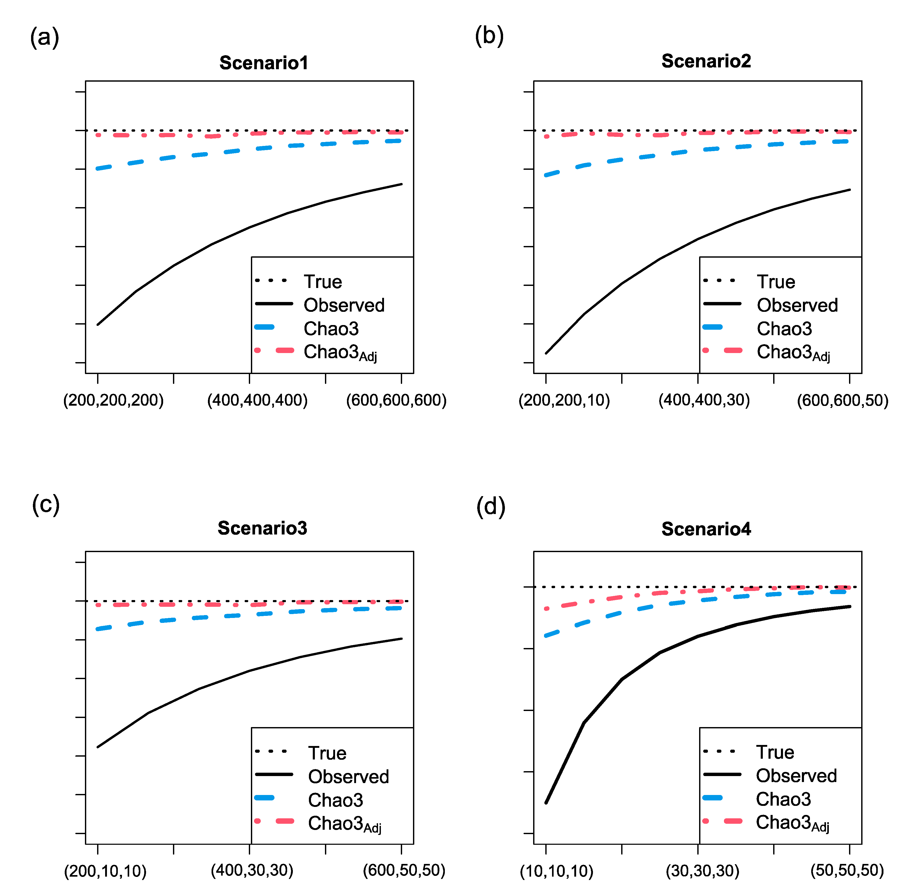
Figure 2. Plot of the true richness of multiple assemblages and the average richness estimates (including observed richness, Chao3, and the adjusted Chao3 (Chao3_Adj)) as a function of sampling effort for four different scenarios. Each scenario involves different combinations of abundance and incidence data: (a) three abundance data, (b) two abundance data and one incidence data, (c) one abundance data and two incidence data, and (d) three incidence data.

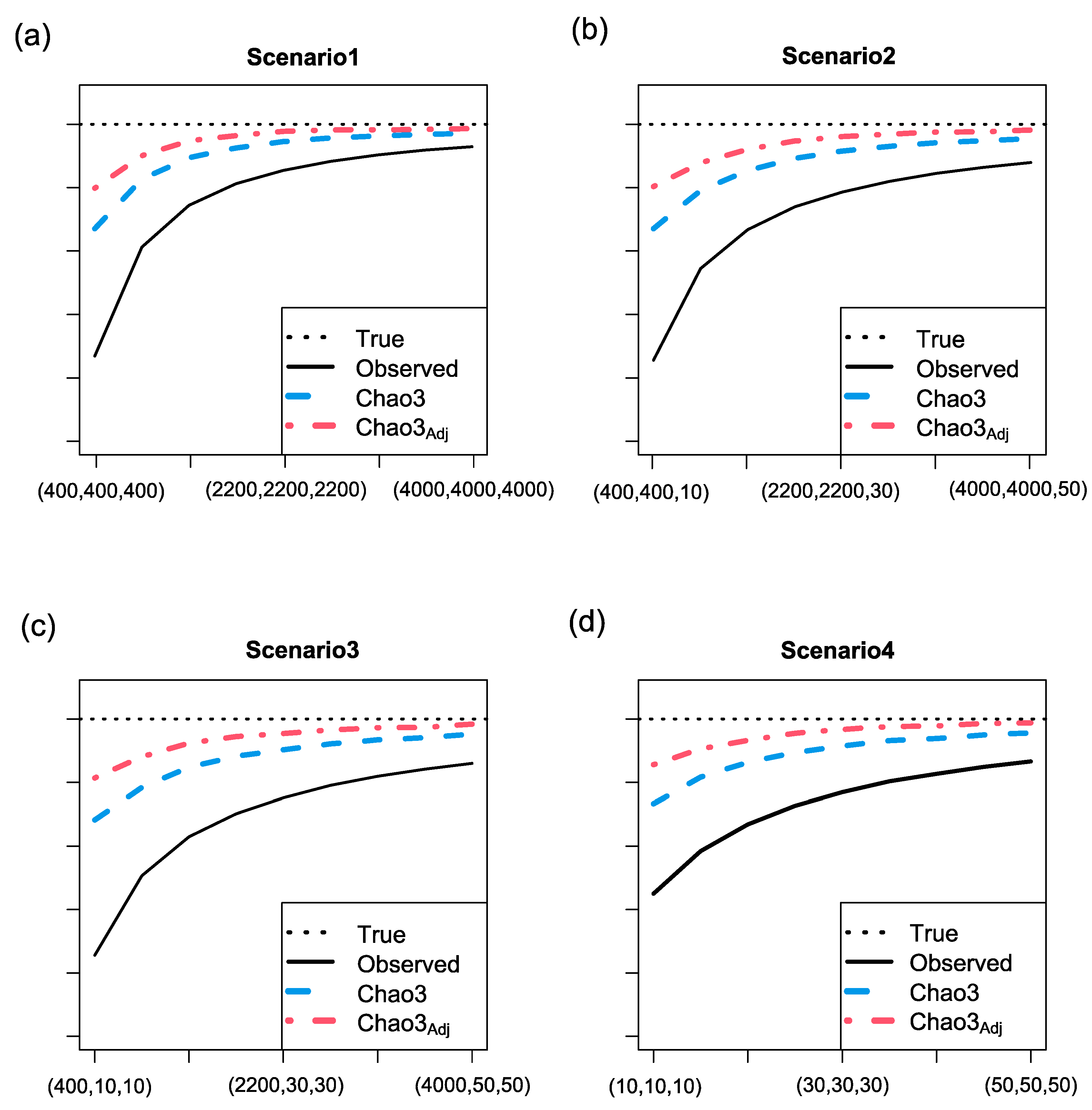
Figure 3. Plot of the true number of moth species and the average richness estimates (including observed richness, Chao3, and the adjusted Chao3 (Chao3_Adj)) as a function of sampling effort for four different scenarios. Each scenario involves different combinations of abundance and incidence data: (a) three abundance data, (b) two abundance data and one incidence data, (c) one abundance data and two incidence data, and (d) three incidence data.

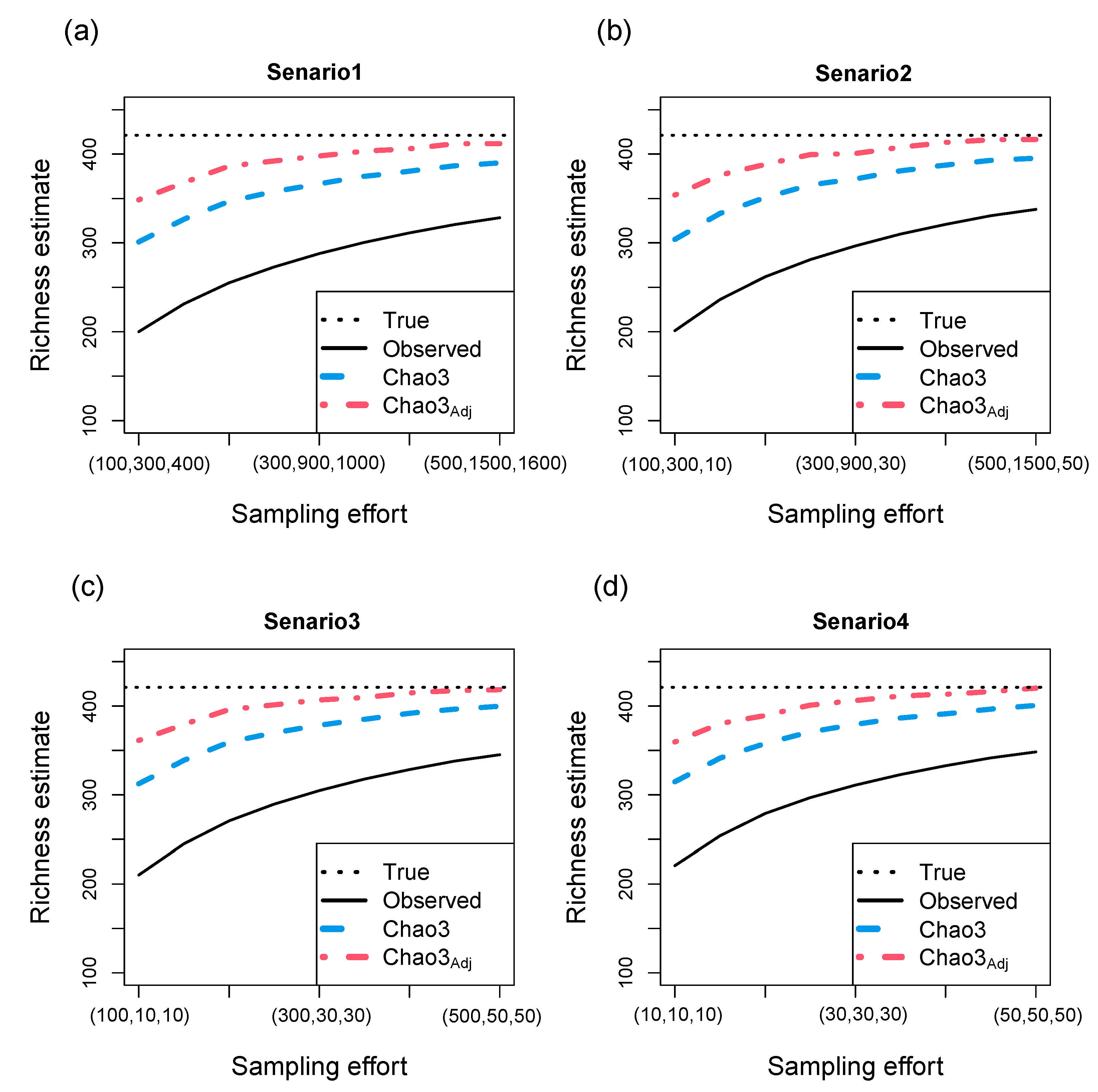
Figure 4. Plot of the true number of xylobiont beetle species and three average richness estimates (including observed richness, Chao3, and the adjusted Chao3 (

C h a o 3_{A d j}

)), as a function of sampling effort for four different scenarios. Each scenario includes different combinations of abundance and incidence data: (a) three abundance data, (b) two abundance data and one incidence data, (c) one abundance data and two incidence data, and (d) three incidence data.

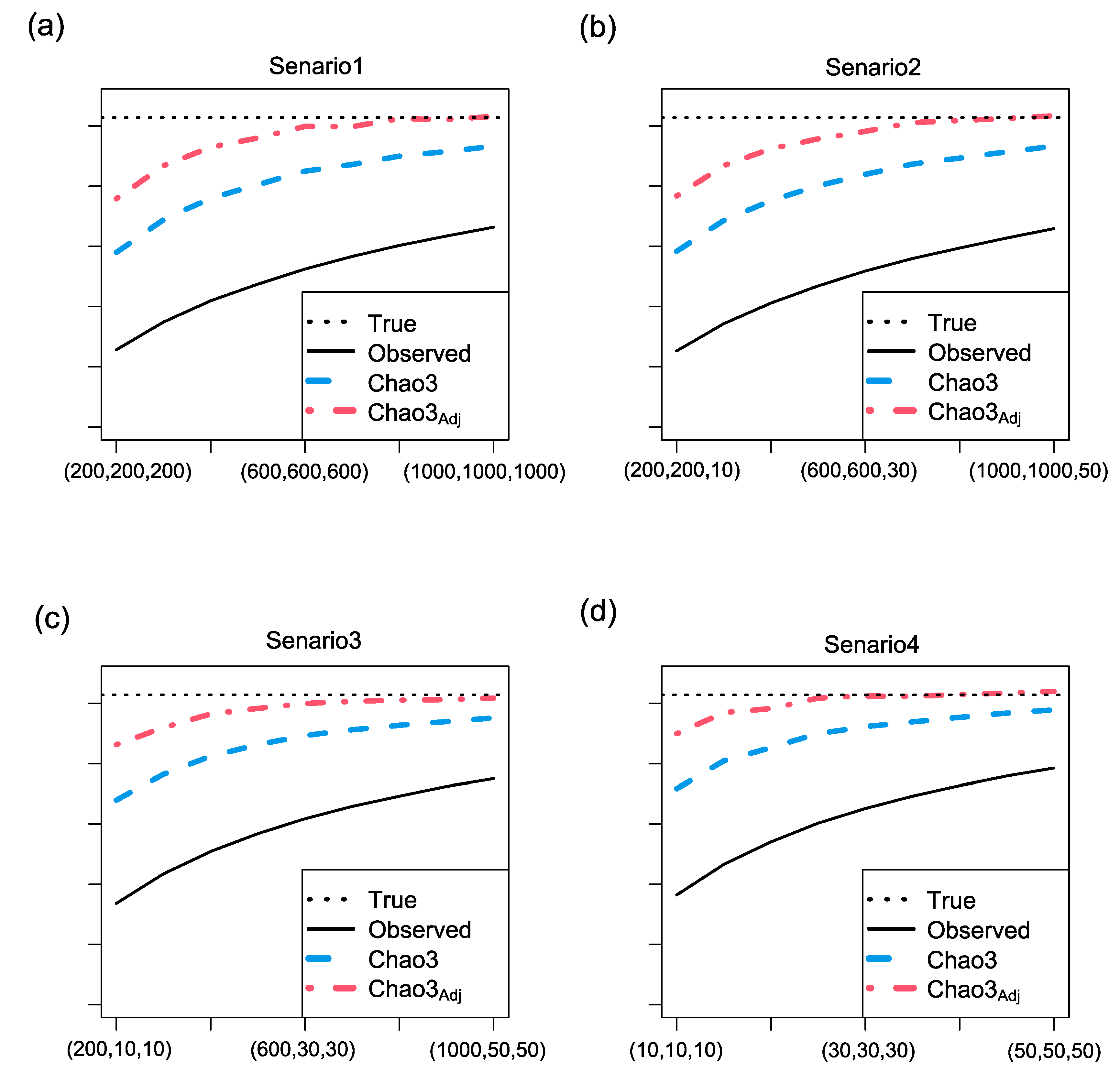
Figure 4. Plot of the true number of xylobiont beetle species and three average richness estimates (including observed richness, Chao3, and the adjusted Chao3 (

C h a o 3_{A d j}

Table 1. The statistical behavior of Chao3 and adjusted Chao3 (Chao3_Adj) are analyzed in four scenarios to estimate the richness of one assemblage. .

Size (Observed richness)	Estimator	Average Estimate	Bias	Sample SE	Average Estimated SE	Sample RMSE	95% CI Coverage Rate
Scenerio1
200, 200, 200 (352.3)	Chao3	557.3	-42.7	37.6	38.7	56.9^†	0.834
200, 200, 200 (352.3)	Chao3_Adj	601.6	1.6^†	71.6	68.2	71.5	0.856^†
400, 400, 400 (480.0)	Chao3	582.1	-17.9	21.4	20.9	27.8^†	0.882
400, 400, 400 (480.0)	Chao3_Adj	601.6	1.6^†	35.7	34.1	35.7	0.87^†
600, 600, 600 (536.2)	Chao3	590.4	-9.6	14.3	13.4	17.2^†	0.91
600, 600, 600 (536.2)	Chao3_Adj	599.9	-0.1^†	22.1	21.5	22.1	0.95^†
Scenerio2
200, 200, 10 (307.9)	Chao3	548.8	-51.2	50.1	46.8	71.6^†	0.804
200, 200, 10 (307.9)	Chao3_Adj	598.2	-1.8^†	93.2	82.1	93.1	0.890^†
400, 400, 20 (441)	Chao3	571	-29	26.3	25.3	39.1^†	0.8
400, 400, 20 (441)	Chao3_Adj	596.3	-3.7^†	45.4	41.9	45.5	0.91^†
600, 600, 40 (513.4)	Chao3	584.9	-15.1	16.9	16.2	22.6^†	0.858
600, 600, 40 (513.4)	Chao3_Adj	598.8	-1.2^†	27.4	26.4	27.4	0.932^†
Scenerio3
200, 10, 10 (330.8)	Chao3	547.9	-52.1	41	41.4	66.3^†	0.786
200, 10, 10 (330.8)	Chao3_Adj	587.1	-12.9^†	74.5	70.7	75.5	0.872^†
400, 20, 20 (460.2)	Chao3	572.1	-27.9	22.6	22.4	35.9^†	0.814
400, 20, 20 (460.2)	Chao3_Adj	593.6	-6.4^†	39.6	36.9	40	0.902^†
600, 40, 40 (538.5)	Chao3	589.3	-10.7	13.2	13.1	17^†	0.902
600, 40, 40 (538.5)	Chao3_Adj	599.8	-0.2^†	20.7	21.3	20.6	0.95^†
Scenerio4
10, 10, 10 (445.0)	Chao3	570.1	-29.9	24.7	24.2	38.8^†	0.808
10, 10, 10 (445.0)	Chao3_Adj	589.4	-10.6^†	41.8	38.2	43.1	0.88^†
20, 20, 20 (540.5)	Chao3	585	-15	11.8	11.8	19.1^†	0.826
20, 20, 20 (540.5)	Chao3_Adj	594	-6^†	18.5	19.2	19.4	0.961^†
40, 40, 40 (583.9)	Chao3	596.3	-3.7	6.1	5.7	7.1^†	0.954
40, 40, 40 (583.9)	Chao3_Adj	599.6	-0.4^†	9.1	10.5	9.1	0.952^†

†

denotes the least bias, lowest RMSE, and closest to 95% coverage. Abbreviations: SE, standard error; RMSE, root mean square error; CI, confidence interval

Table 2. The statistical behavior of

C h a o 3

and adjusted Chao3 (

C h a o 3_{A d j}

) were analyzed in four scenarios to estimate the richness of multiple assemblages.

Table 2. The statistical behavior of

C h a o 3

and adjusted Chao3 (

C h a o 3_{A d j}

) were analyzed in four scenarios to estimate the richness of multiple assemblages.

Sizes (Observed richness)	Estimator	Average Estimate	Bias	Sample SE	Average Estimated SE	Sample RMSE	95% CI Coverage Rate
Scenerio1
500, 500, 500 (457)	Chao3	544.8	-55.2	21.7	20	59.3	0.42
500, 500, 500 (457)	Chao3_Adj	572.9	-27.1^†	38.2	35.5	46.8^†	0.892^†
1000, 1000, 1000 (529.4)	Chao3	573.1	-26.9	13.5	12.8	30.1	0.6
1000, 1000, 1000 (529.4)	Chao3_Adj	587.3	-12.7^†	22.7	22.1	26^†	0.906^†
2000, 2000, 2000 (569.5)	Chao3	589.5	-10.5	9.3	8.3	14.1^†	0.806
2000, 2000, 2000 (569.5)	Chao3_Adj	596.3	-3.7^†	15.2	14.5	15.6	0.972^†
Scenerio2
500, 500, 10 (430.7)	Chao3	518	-82	20.1	20	84.4	0.13
500, 500, 10 (430.7)	Chao3_Adj	545.7	-54.3^†	34.7	35.4	64.4^†	0.786^†
1000, 1000, 20 (502.5)	Chao3	553.2	-46.8	15.2	14.5	49.2	0.306
1000, 1000, 20 (502.5)	Chao3_Adj	572.4	-27.6^†	26.4	25.4	38.1^†	0.858^†
2000, 2000, 400 (547.9)	Chao3	580.2	-19.8	12.9	11.7	23.7	0.694
2000, 2000, 400 (547.9)	Chao3_Adj	593	-7^†	22.1	20.6	23.2^†	0.942^†
Scenerio3
500, 10, 10 (452.6)	Chao3	540.9	-59.1	21.1	19.9	62.7	0.32
500, 10, 10 (452.6)	Chao3_Adj	567.2	-32.8^†	36.8	34.9	49.3^†	0.862^†
1000, 20, 20 (524.9)	Chao3	570.4	-29.6	13.8	13.1	32.6	0.57
1000, 20, 20 (524.9)	Chao3_Adj	584.4	-15.6^†	23.4	22.6	28^†	0.912^†
2000, 40, 40 (566.4)	Chao3	587.4	-12.6	9.1	8.5	15.5	0.782
2000, 40, 40 (566.4)	Chao3_Adj	594.4	-5.6^†	14.5	14.6	15.4^†	0.984^†
Scenerio4
10, 10, 10 (492.4)	Chao3	553.4	-46.6	18	16.6	50	0.41
10, 10, 10 (492.4)	Chao3_Adj	575.3	-24.7^†	31.6	29.3	40.1^†	0.886^†
20, 20, 20 (541.8)	Chao3	576.1	-23.9	12.7	11.6	27	0.642
20, 20, 20 (541.8)	Chao3_Adj	587.3	-12.7^†	21.3	20.1	24.8^†	0.920^†
40, 40, 40 (571.8)	Chao3	588.3	-11.7	7.9	7.6	14.1	0.806
40, 40, 40 (571.8)	Chao3_Adj	594.2	-5.8^†	12.8	13.4	14^†	0.976^†

†

denotes the least bias, lowest RMSE, and closest to 95% coverage. Abbreviations: SE, standard error; RMSE, root mean square error; CI, confidence interval.

Table 3. The summary of three moth samples separately collected from creek, slope and ridge habitats in Costa Rica rain forest[22], and three beetle samples separately collected from Quercus robur, Tilia cordata and Fraxinus excelsior tree species in Leipzig floodplain forest[23].

Moth species data
Habitat	SampleSize	Observed richness	SampleCV	$f_{1}$	$f_{2}$	$f_{3}$	$f_{+ 4}$
creek	461	115	1.86	54	22	9	32
slope	2382	285	2.40	92	47	23	123
ridge	3710	356	2.68	94	59	31	172
Beetle species data
Tree species	SampleSize	Observed richness	SampleCV	$f_{1}$	$f_{2}$	$f_{3}$	$f_{4 +}$
Quercus robur	2205	174	2.72	74	29	10	61
Tilia cordata	1737	198	2.37	92	27	16	63
Fraxinus excelsior	1797	184	3.30	77	31	11	65

Abbreviations: CV: coefficient of variation;

f_{1}, f_{2}, f_{3}

and

f_{4 +}

are respectively the singleton richness, doubleton richness, tripleton richness and the number of species observed more than 3 times in the sample.

Disclaimer/Publisher’s Note: The statements, opinions and data contained in all publications are solely those of the individual author(s) and contributor(s) and not of MDPI and/or the editor(s). MDPI and/or the editor(s) disclaim responsibility for any injury to people or property resulting from any ideas, methods, instructions or products referred to in the content.

© 2023 by the authors. Licensee MDPI, Basel, Switzerland. This article is an open access article distributed under the terms and conditions of the Creative Commons Attribution (CC BY) license (http://creativecommons.org/licenses/by/4.0/).

Copyright: This open access article is published under a Creative Commons CC BY 4.0 license, which permit the free download, distribution, and reuse, provided that the author and preprint are cited in any reuse.

Altmetrics

Downloads

Views

Comments

Subscription

Notify me about updates to this article or when a peer-reviewed version is published.

MDPI Initiatives

Important Links

Choose an area of interest and we will send you notifications of new preprints at your preferred frequency.

Disclaimer

A Richness Estimator Based on Integrated Data

Abstract

Keywords:

Subject:

1. Introduction

2. Materials and Methods

2.1. Sampling distribution model

2.2. Richness estimation for one assemblage based on integrated data

2.2.1. Chao’s lower bound estimators

2.2.2. Extension of Chao’s lower bound estimators for integrated data

2.2.3. Adjusted Lower bound estimator of species richness for integrated data

2.3. Regional richness estimation based on integrated data

2.4. Variance estimation

3. Results

3.1. Simulation study

3.1.1. For individual-based abundance sampling models:

3.1.2. For sample-based incidence sampling models

3.2. Simulation results for richness estimation of one assemblage (a local region)

3.3. Simulation results for richness estimation of multiple assemblages (a large-scale region)

3.4. Using data sets as true assemblages

3.4.1. Moth species data

3.4.2. xylobiont beetle species data

4. Discussion and Conclusion

Data Availability Statement

Conflicts of Interest

Appendix A: Numerical study to show that the expectation of species count of rare frequency in the pooled sample is approximately identical to the probability sum of Poisson distribution.

Appendix B: The summary of the statistical properties of the richness estimators discussed in the text.

Appendix C: Supplementary tables (Table A1 and Table A2)

References

MDPI Initiatives

Important Links

Subscribe