Submitted:
06 July 2023
Posted:
06 July 2023
You are already at the latest version
Abstract
The identification and physical interpretation of quantum correlations, more recently explored beyond entanglement, is not always a simple task. Two assumptions that, at least in principle, should lead to a relatively large dispersion for the observables of a quantum bipartite formed by systems I and II are to assume that; (a) all the possible observables describing the composite are potentially equally probable as outcomes of measurements; and (b) there cannot be concurrence (positive reinforcement) between any of the observables within a given system, meaning all their corresponding operators do not commute. The so-called EPR states are known to observe (a). Here we demonstrate in general terms that they also verify (b). As examples, we discuss three-level systems. Given the character of (a) and (b), one may expect the CHSH correlation for qubits to naturally violate its associated Bell’s inequality (i.e., it would yield values greater than 2) when applied to EPR states. Surprisingly, we show the CHSH contradicts such prediction. This finding emphasizes the subtleties of correlations in quantum mechanics, where the conceivable dispersive interdependence of EPR states observables results counterintuitively in a more limited range of values for the CHSH correlation, not surpassing the nonlocality threshold of 2.
Keywords:
quantum correlations
; EPR states
; entanglement
; Bell's inequalities
; CHSH correlation
1. Introduction
Probability, as formally viewed in stochastic processes (see, e.g., [1]), is a fundamental ingredient to understand countless natural phenomena. For instance, it is ubiquitous in the general framework of classical statistical mechanics. Probability is also a keystone in quantum mechanics, where the concept of probability amplitudes relates to the distribution of outcomes upon measurements. Nonetheless, there are fundamental distinctions between the idea of randomness [2] in classical and quantum physics since probability can have a contrasting character in these two realms [3]. A context where their differences is particularly manifest is in the analysis of correlations of physical quantities [2,4].
Although many restrictions may apply [5], correlations can be used as an measure of the degree of determinism/randomness in a system. Indeed, certain situations might be relatively easily to pinpoint. On the one hand, if there is a well-behaved mapping between a and b (with a and b possible values for bona fide observables A and B describing a problem1) — e.g., and r in a classical Keplerian orbit — the correlation is “perfect” and there should be a fully deterministic causation between them. On the other hand, if a specific value for A determines a range of allowable values for B as well as their frequencies of occurrence (with the same being true for A regarding B), this would indicate a stochastic connection between A and B. So, at least in principle one could infer a joint probability for A and B, allowing to define a proper correlation function for A and B, .
But as already mentioned, will display different features if resulting from either classical or quantum processes 2. Quantum are often more general than classical correlations [4,9,10] and in some cases stronger [11,12,13], for example, creating scalings (due to entanglement) in many-body systems which are of course classically absent [14,15]. Actually, there are distinct types of quantum correlations [9], from the most basic — associated to the quantum formalism itself, which we simply call `quantum’ — to those presenting an increasing order of restrictness, namely, entanglement, steering and nonlocality, Figure 1.
In brief, entanglement can be thought of as the primordial quantum correlation since it includes all possible forms of interrelations in pure bipartite states. When a composite state , with and the Hilbert space of systems I and II, cannot be written as the direct product , for and , we say that is entangled. A second, greater, interaction between systems I and II is that in which the state of one of them (e.g., I) can be driven or steered through measurements on the other (e.g., II); nevertheless the contrary does not hold true. In such inseparability context, the composite system exhibits a steering correlation (reviews in [9,16,17]). All steered systems are entangled, but not all entangled systems are steered. Finally, suppose we measure the observable A for system II and C for system I (with I and II assumed away apart), obtaining respectively a and c. In quantum mechanics, one finds that usually the joint probability . The explanation is that the quantum world is nonlocal, a notion heavily criticized by the famous EPR (Einstein, Podolsky, Rosen) paper [18]. An alternative would be to assume that quantum mechanics is incomplete, i.e., there exist local hidden variables inaccessible by the theory. In Bell’s groundbreaking work [19], it has been demonstrated that then and some inequalities for the associated quantum correlations should be observed. However, the local hidden variables have been ruled out through concrete experiments [20,21,22,23,24,25,26,27,28,29] showing the violation of the Bell’s inequalities. Thus, in opposition to the EPR local realism, nonlocality is inherent to quantum mechanics and indeed its most restrictive correlation [9,30].
A rather significant example of Bell’s inequality for qubits (two levels systems) is the so called CHSH’s [31]. Consider an ensemble of a composite formed by systems I and II. For all copies, I and II are put apart (conceivably without disturbing the original properties we shall measure). So, detectors 1 and 2 can infer certain observables for I ( and , whose results are denoted as e ) and II ( and , of results e ), Figure 2. From appropriate averages we can calculate the CHSH correlation function — explicit expressions are given in Section 5. For arbitrary observables X’s and Y’s, local hidden variables would dictate . But quantum mechanics also allows , corresponding to a Bell’s inequality violation.
All the previous discussion eventually might give the wrong impression that to identify and classify quantum correlations is a rather straightforward task. In fact, from a technical point of view this is not usually the case [9,32,33,34]. But perhaps more surprisingly, in certain instances even a conceptual intuition about correlations can fail in the quantum context. Consider the observables for I and for II, with . For any j the allowed outcomes are the same, and . Also, is a quantum correlation function of these possible observables considered in pairs . With the exception of too specific functional forms for , typically we could anticipate a greater (smaller) dispersion for to be related to a weaker (stronger) interdependence among . To be more concrete, let us presume the two conditions: (a) Regardless of j, the corresponding are all equally likely to describe the composite system state, i.e., in an ensemble sense we have an uniform distribution for these values so that any pair n of contributes with a same probability . Hence, for and fixed N, this assumption maximizes the normalized entropy (note that is well-defined even in the hypothetical limit of ). (b) There are no reinforcement dependence between the ’s and between the ’s. On the contrary, to know () precludes to know with certainty the value of (), . This is the physical consequence of the non-commutation, and , of the corresponding self-adjoint operators for the observables and in quantum mechanics. Therefore, given (a) and (b) we could expect a broader range of variation for . So, for being the CHSH (thence with ), presumably we would have the non-observance of the Bell’s inequality.
The arguments3 in [18] were completely based on particular bipartite ’s, the EPR states which do verify the assumption (a) (see next for detailed definitions). The conclusions in [18] — hence, somehow indirectly the structure of these ’s — motivated the investigations in [19] (refer also to [36,37]). But as aforementioned, incidentally local realism has been overturned by testing the Bell’s inequalities for arbitrary ’s.
In the present contribution we prove generally that the ’s also comply with the assumption (b). So, one could speculate the CHSH inequality to be overruled when considered for EPR states. We check this possibility by calculating only for observables (of , so essentially qubits) associated to . We find that . This result is a bit unforeseen taking into account the above ponderations. Moreover, it clearly typifies the subtleties of correlations in quantum mechanics, with the seemingly high dispersive interdependence of EPR states observables given rise to a more limited interval of values for , not exceeding the nonlocality threshold of 2.
The paper is organized as the following. We review important aspects of EPR states in Section 2. We demonstrate the condition (b) for EPR states in Section 3. We exemplify the results of Section 3 for three levels systems in Section 4. We show that EPR states do not violate Bell inequalities in the case of CHSH correlations in Section 5. Final remarks and conclusion are drawn in Section 6. More technical analysis are left to the Appendices.
2. Some Key Aspects in Forming and Measuring EPR States
Here we review the basic characteristics of EPR states [38], essentially those considered in the original work by Einstein-Podolsky-Rosen [18]. A much more general and rigorous definition for finite dimensional systems can be found in [39,40] (for infinite-dimensional spaces, see [41,42]). Furthermore, we briefly discuss: the kind of measurements one can perform on , the associated possible outcomes, and the consequent state reductions.
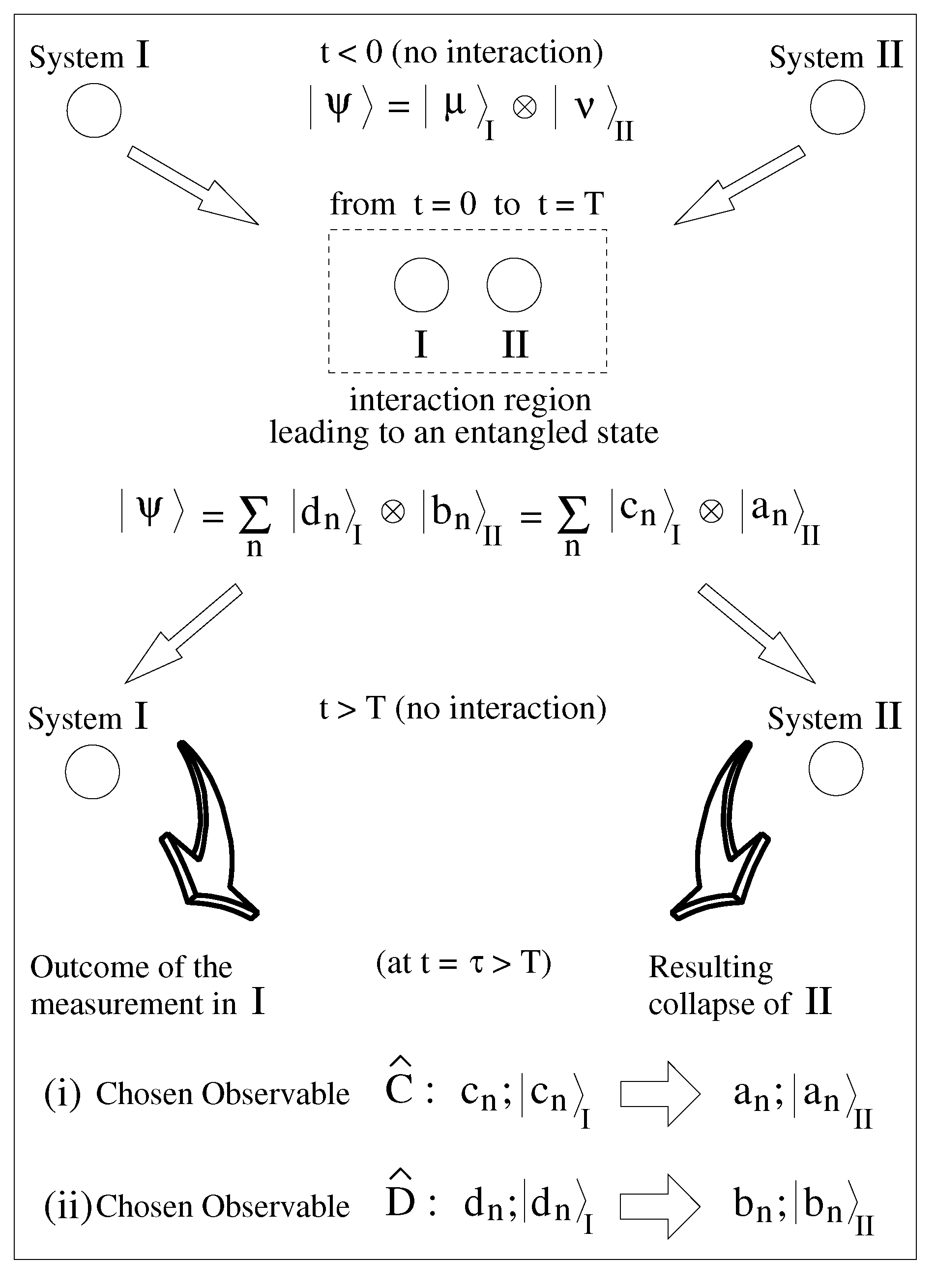
The main relevant steps in the preparation and posterior measurement of are schematically depicted in Figure 3. Initially (), one has two non-interacting systems I and II, with their composite state being simply the direct product of the individual states of I and II. Then, during the time interval , I and II are brought to interact in such way to quantum correlate certain physical observables pertaining to I (say C; associated to the Hermitian operator with eigenvalues ) with some of those pertaining to II (say A; associated to with ), yielding the entangled state (we assume ). Next, for , I and II are somehow put sufficiently away so to cease any eventual mutual influence between the two systems. In other words, the type of interaction normally described by a potential in the Schrödinger equation — coupling the systems I and II degrees of freedom — should be null. However, one must guarantee that regardless the separation procedure and the subsequent dynamics (for ), the attained entanglement (along ) between I and II are maintained. Obviously, this until an eventual measurement at any . Hence, this last process would not alter the components of corresponding to the eigenvectors of I and of II, or ()
In Eq. (1), and denote how other observables, distinctly from C of I and A of II, will evolve in time given that the systems no longer interact.
If by means of measurements we aim to assess only the correlated quantities C and A, the information given by and are not really relevant. Thus, one can drop these explicit dependences in Eq. (1), just written for . We mention that it is a common practice in the analysis of EPR states [38,39]: (i) To suppose maximally entangled states, i.e., all in being equally probable, namely, for any n to assume that . (ii) To disregard eventual relative phases by trivially reincorporating them into the states definition, or . Thus, the existence or not of phases multiplying the eigenvectors is totally irrelevant for all our general results next.
A second fundamental feature of a EPR state is that (with , but prior to any measurement) can be written in the following distinct ways
where the set () is composed by the eigenvectors of (), or
Therefore, from Eq. (2) we have that from a measurement performed only on I at — determining the observable C (D) — we should obtain complete knowledge about the value of A (B) for II, Figure 3. In fact, if afterwards () we test system II for A (B), we should find exactly this previously inferred value.
The last feature defining an EPR state is to have for the observables A and B — associated to system II, cf. Eq. (2) — operators which do not commute, i.e., . Actually, an important and involved issue related to this property is, given an EPR state, to determine all its associated pairs of non-commuting observables [40]. We shall remark that was a key assumption in [18], in the attempt to show (of course misguidedly; see a summary of many valid objections to the EPR arguments in [35] as well as in the refs. therein) that quantum mechanics is incomplete.
3. A Necessary Condition for EPR States: The Observables Are Pairwisely Associated to Non-Commuting Operators
Hereafter we assume that for the composed systems (refer to Eq. (1)), . Note that and distinguishes I from II. On the other hand, all the specific aspects [43] we wish determining for our individual systems (either I or II) are described by a proper separable Hilbert space of dimensions N, finite or infinite, spanned by a countable, i.e., discrete, basis (see Eq. (4) below). The reasons are twofold.
First, EPR-like states have been vital to test certain fundamental predictions of QM, e.g., motivating the development of the Bell inequalities [19,36]. But although some theoretical proposals [44], and even devised experimental arrangements [45,46,47], are based on continuous variables (for a review, see [48]), historical breakthroughs [20,21,22,23,24,25] and recent loophole-free measurements [26,27,28,29,49] consider discrete observables. Second, the spectrum theorem for self-adjoint operators — relevant to determine suitable basis for — holds true in very general terms [50]. However, to establish solid grounded properties of transformations (similar to those presented in Section 3.1) between continuous basis might demand extra technicalities, going beyond the scope of this contribution. For instance, for continuous basis associated to operators such as position and momentum, one should work with generalized eigenvectors in a rigged Hilbert space [51].
As quantum observables we consider linear self-adjoint — or Hermitian, the usual jargon in physics — operators, whose domains are the whole (or linear subsets of which are dense in if the self-adjoint operators are unbounded [52,53], Appendix A). Also, for our goals it is not necessary to explicit address formal constructions of the join probability measures associated to any assessment of observables, e.g., as rigorously done in [39]. Pragmatically, we just suppose fairly well-established definitions (refer to [39]), consistent with actual procedures in concrete measurement realizations [20,21,22,23,24,25].
For and being the set of eigenvectors of and and representing orthonormal basis (ONB) of , the basis change are implemented through (for N finite or infinite)
To derive the main result of the next Sec., we will rely on some features of such unitary matrix — which are dependent on the commutation relation of and and discussed in the Appendix A. We also leave to the Appendix A considerations about appropriate self-adjoint operators and to represent observables for EPR states.
3.1. Correlations in the Observables of EPR States
From the above discussions and the remarks in Section 2, for the systems I and II described by EPR states in Eq. (2), we can concentrate on the “reduced” Hilbert space . Moreover, for the self-adjoint operators , , , (see Eq. (3)), we assume the features described in the Appendix A.2 and that and ( and ) are defined on I (II). Thus, the set of eigenvectors and , respectively of and , are suitable ONBs for . The same is true regarding and ) (of and ) with respect to . We also recall that .
Next, by inserting the second relation in Eq. (4) into the second equality in Eq. (2), we get
Comparing Eq. (5) with Eq. (2), we must have (recalling that is an ONB)
Hence, from Eq. (6) we see that up the complex conjugation of the elements of (an operation which certainly should not change their matrix structural relations), the basis transformation is fully akin to . In other words, Eq. (6) has exactly the same functional form of the mapping between and .
But the matrix — hence also — represents a change of basis associated to non-commuting operators, and . So, according to Appendix A.2 it cannot be transformed into an identity, or more generally in a permutation, matrix. In the Appendix A.3 we illustrate such universal fact considering the basis transformations of a spin- system in arbitrary directions. So, , cannot commute, otherwise it would be possible to find a basis where they are simultaneously diagonal leading to (or ), which is a contradiction.
Thus, if a state can be expanded as in Eq. (2), for the different basis related to the Hermitian operators , , , , and , we conclude that necessarily . As far as we know, this rather straightforward property of EPR states has surprisingly gone unexplored in the literature, even though it is implicit in particular contexts, like in the Bohm construction of EPR states [54] and in the Bohr’s response [55] to the EPR paper [18].
4. An Explicit Example: Three Levels System
To illustrate the previous discussion, we assume such that the systems can be described in terms of three components angular moment states. The procedure here, although implemented to a particular situation, also exemplifies how to generate different expansions for a EPR state .
In this case, the equivalent to the Pauli matrices read (with the usual direction association: 1 for x, 2 for y, 3 for z)
where for the permutation symbol of and () for . Further, we have for the eigenstates ( and )
For the basis transformation (with ), we find
whereas for (with and ), we get
For any w and , obviously and .
From the above one finds , , . Furthermore, for our purposes next it is useful to consider the notation meaning (notice the complex conjugation “” of ). Hence
- •
- (1,2) :
- •
- (2,1) :
- •
- (1,3) :
- •
- (3,1) :
- •
- (2,3) :
- •
- (3,2) :
In this way, in all situations with , results in an eigenvector of either , or , having the general form , where:
(i) , but always with ,
(ii) ,
(iii) .
Now, let us suppose the state (for arbitrary)
then for any we have
For , the operators and for system II do not commute. Also in such case, necessarily will be one of the eigenvalues (eventually multiplied by a phase ) of the operator , which according to the condition (i) above does not commute with .
Thence, for f an one-to-one index function from to and integer numbers, we find that
so that is an EPR state (note we could simply relabeling ) and, as it should be, displays all the necessary properties regarding the non-commutation of the associated observables since and .
As a last example we discuss a degenerated case. We should mention that using the general expressions in [56], it is straightforward to engender Hermitian matrices displaying degenerated eigenvalues. Thus, suppose the eigenvalues (so , ) of the eigenvectors of
We set
Changing the basis from to , as done in Eq. (12), and from the explicit form of , we get (for , thus assuming the values 1,-1,0 for , respectively)
for of eigenvalues (so , ) such that , with
5. EPR Observable Correlations for Qubits Do Not Violate the Bell Inequalities
As it should become clear from our previous analysis, EPR states display a rather unusual link between their observables. They are pairwisely incompatible, namely, considering Eq. (2) we cannot simultaneously determine A and B for II and C and D for I. So, an interesting question is which are the possible values for the CHSH correlation function [31], obtained only from EPR states.
Assuming the EPR-like state in Eq. (2), let with the possible eigenvalues of ) being (so , ). For simplicity, we disregard eventual relative phases between the states. Nonetheless, we emphasize that introducing them through, , , and , does not change the following results. Thus
The transformation from the basis to is given by an arbitrary unitary matrix , whereas from to is given by the complex conjugated of (cf., Eqs. (5)–(6)), or . Using an appropriate parameterization for U(2) matrices (see, e.g., [57]), we generally have
with complex numbers such that and . Moreover, we suppose so that (see Appendix A.3). Thus,
To obtain (as well ) and (as well ) we consider in Eq. (22) given, respectively, by the first and second expansion in Eq. (18). So, straightforwardly we find
For and we get
Now, using Eq. (20) into Eq. (24)
Finally (for , , )
Analyzing all the combinations (i.e., , or , ) for , , , one realizes that the only possibilities for are
Hence, if we calculate for any set of observables for which the state has the EPR structure, always . However, the Bell’s inequalities violation in the CHSH construction corresponds to (in fact, [58]).
The above finding is thus somewhat intriguing. The violation of the Bell inequalities [19,36] for a quantum system overturns the EPR claims that quantum mechanics is incomplete [37]. Actually, many breakthrough experiments have clearly demonstrate the existence of quantum correlations violating the Bell’s inequalities [20,21,22,23,24,25,26,27,28,29]. But the special correlations in EPR states seem to be of a different nature. Indeed, by probing solely the EPR observables (here qubits) in a CHSH-like experiment, surprisingly one would not be able to discard hidden local variables.
6. Final Remarks and Conclusion
Universal quantum correlations — thus, much beyond entanglement — are notoriously more diverse and conceptually more complex than the classical counterpart. Mostly because of that, they tend to deceive our common sense expectations about their trending behavior. However, this is just a natural consequence of the involved way in which obervables are interrelated in certain specific quantum states. In the present work, we have analyzed one of these special ’s, bipartite EPR states.
For EPR states, it is prominent that all the associated observables are equally probable as the outcome results of measurements in a composite formed by systems I and II. But more than that, in the present work we have established that if can be expanded, say, in terms of eigenvectors either for the observables C (of I) and A (of II) or D (of I) and B (of II), then necessarily C is incompatible with D, and A is incompatible with B. In other words, for the corresponding self-adjoint operators it follows that and . For concrete examples, we have analyzed EPR states in the case of three-level systems
Given on the one hand the equiprobability, for any , for the observance — through experiments — of pairs of values ( or ( or etc., and on the other hand, a non-concurrence of for I and for II, then we have a considerable dispersion for the EPR observable values. Hence, for the case of qubits (), supposing the CHSH correlation function only for EPR states, one would foresee the violation of the associated Bell inequality, i.e., . But on the contrary, the we have explicitly shown that .
This finding emphasizes the intricacies of correlations in quantum mechanics. Indeed, an apparent strong dispersive interdependence of EPR states observables ends up leading to a more limited range of values for the important CHSH correlation in qubits.
Finally, a natural question relates to a possible extension of the present results to higher-dimensional systems, i.e., for . For such a type of analysis, it is first necessary to make a generalization of the Bell’s inequalities, in particular, of the CHSH correlation. In fact, some interesting proposals have already been discussed in the literature [59,60,61]. Second, irrespective of the exact analytic form of a generalized , the computation idea should be the same as that in Section 5. In this way, it would require unitary matrices of order . Given that a U(N) has free parameters, general analytic calculations tend to be laborious. Presently, we are studying some concrete cases, and hopefully the results will appear in due course.
Author Contributions
Conceptualization, M.G.E. da Luz; methodology, D.F. Orsini; software, D.F. Orsini and L.R.N. Oliveira; validation, D.F. Orsini and L.R.N. Oliveria; formal analysis, D.F. Orsini and L.R.N. Oliveira; investigation, D.F. Orsini, L.R.N. Oliveira and M.G.E. da Luz; writing—original draft preparation, M.G.E. da Luz; writing—review and editing, D.F. Orsini, L.R.N. Oliveira and M.G.E. da Luz; supervision, M.G.E. da Luz; project administration, M.G.E. da Luz; funding acquisition, M.G.E. da Luz. All authors have read and agreed to the published version of the manuscript.
Funding
This work was supported in part by the project “Efficiency in uptake, production and distribution of photovoltaic energy distribution as well as other sources of renewable energy sources” (Grant No. 88881.311780/2018-00) via CAPES PRINT-UFPR. Research funding is also provided by the Brazilian agency CNPq through Grant No. 304532/2019-3 and Grant No. 404577/2021-0 (Universal). D.F. Orsini and L.R.R. Oliveira acknowledge CAPES for the PhD fellowship program.
Acknowledgments
We would like to thank fruitful and elucidating discussions with A. M. Ozorio de Almeida, R. M. Angelo, M. W. Beims, N. P. Neto, A. D. Ribeiro, B. A. Mello and L. S. Schulman.
Conflicts of Interest
The authors declare no conflict of interest.
Abbreviations
The following abbreviations are used in this manuscript:
| EPR | Einstein-Podolsky-Rosen |
| CHSH | Clauser-Horne-Shimony-Holt |
| ONB | Orthonormal basis |
Appendix A. Transformations between Eigenbasis Associated to Commuting and Non-Commuting Operators
In this Appendix we discuss some important characteristics of transformations between countable basis of a separable Hilbert space .
We start addressing the dimensions of the unitary (i.e., ) in Eq. (4). For finite N, the transformation matrix features are simple rooted in standard linear algebra. However, for the infinite case the issue is if the corresponding is mathematically well-defined. In other words, one should assure that the typical matrix operations, as multiplication, remain valid for (at least to ensure unitarity).
The answer is positive provided: (i) we are dealing with suitable ONBs for (see below); and (ii) the elements of essentially represent inner products between basis eigenvectors, namely, and , refer to Eq. (4). Then, Lemma 1.13 in [62] (see also [63]) guarantees that , , , and are all meaningful and that and in Eq. (4) are unitary regardless of N. For further details, we cite comprehensive studies in the literature about infinite-by-infinite unitary matrices [64], infinite matrix representation theory of operators in Hilbert spaces [65,66] — including the unbounded case [67] — and transformations between infinite ONB’s [63,68].
Appendix A.1. The Observables Assumed for EPR States
For a EPR state in a given Hilbert space , a key point is the special ways can be expanded in terms of eigenbasis of pertinent observables (cf., Eq. (2)). Thence, an important question is whether or not these eigenbasis can properly span . In the following we summarize only certain facts about the spectrum of a general self-adjoint operator , relevant to settle the query. For a throughout account on the subject we suggest [65,69,70] (and in the particular context of quantum mechanics we mention [71,72,73]).
A real iff the resolvent is not a bounded operator in the full domain of . is given by the union [74] of the not necessarily disjoints sets , , , respectively, pure point, absolute continuous, and singular continuous spectra. Vectors associated to each one of these sets (see, e.g., [65,69]) form three mutually orthogonal subspaces, , , and , all invariant under . Then, can be written as the direct sum
For usual quantum physics Hamiltonians, the pure point and absolute continuous parts of the spectrum are associated, respectively, to bound and scattering states [75,76,77]. Much less common is a non-empty [78,79,80], generally related to special Hamiltonians, e.g., with random or `bump’ [78] potentials. In such case, the singular continuous spectrum accounts for phenomena like Anderson localization (see [76] and refs. therein).
In our present context, according to Eqs. (2) and (3) appropriate values for the observable A of a EPR state are the a’s in the spectrum set . Indeed, we say the eigenvalue a belongs to if there is at least one (eigenvector) in the domain of satisfying . Since is a subset of [81], all the eigenvectors are in the subspace . For finite (a typical example being the spin-1/2 spinor space, see Appendix A.3), .
The multiplicity (in quantum mechanics, degeneracy) of an eigenvalue a is the dimension of its eigenspace. In other words, the degeneracy of any a is the number of distinct eigenvectors solving the corresponding eigenvalue equation. We have that only if its multiplicity is finite. For instance, for an electron in a constant magnetic field, we have the well known discrete Landau levels. However, the full wave function has a plane wave component, making the Landau levels infinite degenerated and the states not in , so formally not true eigenstates in [73,82].
Lastly, for a self-adjoint (with not null), its set of eigenvectors forms a basis for if:
As illustrations, for (ii) we mention a not too singular attractive potential (like the Hydrogen atom [86]). Then, would correspond to the restriction [87] of the associated Hamiltonian to the subspace of the bound states [72,86]. For (iii), we can cite as Hamiltonians of confining potentials, such as the harmonic oscillator [87]. For non-analytic potentials, e.g., the infinite square well, self-adjoint extension techniques also can lead to proper [88,89,90].
Appendix A.2. The Structure of the Transformation Matrix Γ
For both , one of the cases (i)–(iii) in the Appendix A.1 and ()
the sets and are normalized basis of the Hilbert space . In the spin-1/2 Bohm’s version [54,91] of the EPR original construction [18], or in the general rigorous definition of EPR states [39] (for infinite-dimensional spaces see [41,42]), all the basis discussed are orthonormalized. This is straightforwardly the case for and if the set of eigenvalues and are non-degenerated. On the other hand, eigenvectors belonging to a same eigenvalue in principle do not need to be mutually orthogonal. However, relying on the spectral decomposition theorem for self-adjoint operators on linear Hilbert spaces [65], we always can use the Gram-Schmidt orthogonalization procedure, obtaining a complete orthonormal basis ONB for . Thus, without loss of generality we can assume and as ONBs.
We now consider two possible situations for the operators and and analyze the structure of the transformation matrix in Eq. (4). For so, we shall rely on well known results about diagonalization of self-adjoint operators, a subject discussed in many quantum mechanics textbooks (for a particularly comprehensive treatment see [92]):
- and commute: (1) The operators have common eigenvectors. (2) So, in a basis in which one is diagonal, say , is block diagonal with the distinct blocks having dimensions (all finite, see Appendix A.1) equal to the multiplicity of the different eigenvalues. (3) But from the previous remarks about spectra decomposition, these blocks always can be put in a diagonal form. Therefore, there is at least one basis simultaneously diagonalizing and . As consequence of (3), in Eq. (4) can be reduced to an identity matrix of size N. Actually, in general is a permutation matrix once in Eq. (4) we can have for some subsets of indices . Nonetheless, given that for any permutation matrix , a trivial relabeling of one of the basis indices, say , gets into .
- and do not commute: (4) There are no common eigenvectors and thus no basis can simultaneously diagonalize and . (5) In this way, the matrix may (due to occasional symmetries associated to and ) or may not display a block diagonal format. However, in either situation itself or its eventual diagonal blocks cannot be turned into identity matrices, once then it would imply the existence of mutual eigenvectors, violating (4).
An illustration of the above is presented in the Appendix A.3 for spin- systems.
Appendix A.3. The Basis Transformation Matrix for Spin-1/2 Systems in Arbitrary Directions
For , , and , the first, second, and third Euler angles, the spin- system component in the direction is represented by the operator () [93]
The eigenvectors of read [93]
Thus, a basis transformation from to , written as
leads to an unitary matrix whose elements are (with , , and )
From a direct analysis of Eq. (A3), one finds that can be reduced to (or its associated permutation, Appendix A.2) only for those combinations of the angles , , , corresponding to (and so we can set ). Note this is indeed a consequence of to vanish only if (the minus signal taking into account cases like and , for which and ).
Therefore, for and not parallel or anti-parallel, the structure of is that of transformations between ONBs associated to non-commuting operators, exemplifying our general result in the particular case of a spin- problem.
References
- Brémaud, P. Probability theory and stochastic processes, 1st ed.; Springer Cham: Berlin, Germany, 2020. [Google Scholar]
- Knill, E.; Zhang, Y.; Bierhorst, P. Generation of quantum randomness by probability estimation with classical side information. Phys. Rev. Res. 2020, 2, 033465. [Google Scholar] [CrossRef]
- Beltrametti, E. G. Classical versus quantum probabilities. In Chance in physics: foundations and perspectives; Bricmont, J., Ghirardi, G., Dürr, D., Petruccione, F., Galavotti M., C., Zanghi, N., Eds.; Springer: Berlin, Germany, 2001; pp. 225–232. [Google Scholar]
- Gallego, R.; Masanes, L.; De La Torre, G.; Dhara, C.; Aolita, L.; Acín, A. Full randomness from arbitrarily deterministic events. Nat. Commun. 2013, 4, 2654. [Google Scholar] [CrossRef]
- Pearl, J. Causality: models, reasoning and inference, 2nd ed.; Cambridge University Press: Cambridge, UK, 2009. [Google Scholar]
- Modi, K.; Paterek, T.; Son, W.; Vedral, V.; Williamson, M. Unified view of quantum and classical correlations. Phys. Rev. Lett. 2010, 104, 080501. [Google Scholar] [CrossRef]
- Adesso, G.; Datta, A. Quantum versus classical correlations in Gaussian states. Phys. Rev. Lett. 2010, 105, 030501. [Google Scholar] [CrossRef]
- Maziero, J.; Werlang, T.; Fanchini, F. F.; Céleri, L. C.; Serra, R. M. System-reservoir dynamics of quantum and classical correlations. Phys. Rev. A 2010, 81, 022116. [Google Scholar] [CrossRef]
- Adesso, G.; Bromley, T. R.; Cianciaruso, M. Measures and applications of quantum correlations. J. Phys. A 2016, 49, 473001. [Google Scholar]
- Guo, Z.; Cao, H.; Chen, Z. Distinguishing classical correlations from quantum correlations. J. Phys. A 2012, 45, 145301. [Google Scholar] [CrossRef]
- Xu, J.; Xu, X.; Li, C.; Zhang, C.; Zou, X.; Guo, G. Experimental investigation of classical and quantum correlations under decoherence. Nat. Commun. 2010, 1, 7. [Google Scholar] [CrossRef]
- Branciard, C.; Gisin, N.; Pironio, S. Characterizing the nonlocal correlations created via entanglement swapping. Phys. Rev. Lett. 2010, 104, 170401. [Google Scholar] [CrossRef]
- Fritz, T. Beyond Bell’s theorem: correlation scenarios. Phys. Rev. Lett. 2012, 14, 103001. [Google Scholar] [CrossRef]
- De Chiara, G.; Sanpera, A. Genuine quantum correlations in quantum many-body systems: a review of recent progress. Rep. Prog. Phys. 2018, 81, 074002. [Google Scholar] [CrossRef]
- Frérot, I.; Fadel, M.; Lewenstein, M. Probing quantum correlations in many-body systems: a review of scalable methods. arXiv preprint:2302.00640 2023. [Google Scholar]
- Cavalcanti, D.; Skrzypczyk, P. Quantum steering: a review with focus on semidefinite programming. Rep. Prog. Phys. 2016, 80, 024001. [Google Scholar] [CrossRef] [PubMed]
- Uola, R.; Costa, A. C. S.; Nguyen, H. C.; Gühne, O. Quantum steering. RMP 2020, 92, 015001. [Google Scholar] [CrossRef]
- Einstein, A.; Podolsky, B.; Rosen, N. Can quantum-mechanical description of physical reality be considered complete? Phys. Rev. 1935, 47, 777. [Google Scholar] [CrossRef]
- Bell, J. S. On the Einstein Podolsky Rosen paradox. Physics 1964, 1, 195–200. [Google Scholar] [CrossRef]
- Aspect, A.; Grangier, P.; Roger, G. Experimental realization of Einstein-Podolsky-Rosen-Bohm gedankenexperiment: a new violation of Bell’s inequalities. Phys. Rev. Lett. 1982, 49, 91–94. [Google Scholar] [CrossRef]
- Aspect, A.; Grangier, P.; Roger, G. Experimental test of Bell’s inequalities using time-varying analyzers. Phys. Rev. Lett. 1982, 49, 1804–1807. [Google Scholar] [CrossRef]
- Tapster, P. R.; Rarity, J. G.; Owens, P. C. M. Violation of Bell’s inequality over 4 km of optical fiber. Phys. Rev. Lett. 1994, 73, 1923. [Google Scholar] [CrossRef]
- Tittel, W.; Brendel, J.; Zbinden, H.; Gisin, N. Violation of Bell inequalities by photons more than 10 km apart. Phys. Rev. Lett. 1998, 81, 3563. [Google Scholar] [CrossRef]
- Weihs, G.; Jennewein, T.; Simon, C.; Weinfurter, H.; Zeilinger, A. Violation of Bell’s inequality under strict Einstein locality conditions. Phys. Rev. Lett. 1998, 81, 5039. [Google Scholar] [CrossRef]
- Aspect, A. Quantum mechanics: to be or not to be local. Nature 2007, 446, 866–867. [Google Scholar] [CrossRef] [PubMed]
- Hensen, B.; Bernien, H.; Dréau, A. E.; Reiserer, A.; Kalb, N.; Blok, M. S.; Ruitenberg, J.; Vermeulen, R. F. L.; Schouten, R. N.; Abellán, C.; et al. Loophole-free Bell inequality violation using electron spins separated by 1.3 kilometers. Nature 2015, 526, 682–686. [Google Scholar] [CrossRef]
- Shalm, L. K.; Meyer-Scott, E.; Christensen, B. G.; Bierhorst, P.; Wayne, M. A.; Stevens, M. J.; Gerrits, T.; Glancy, S.; Hamel, D. R.; Allman, M. S.; et al. Strong loophole-free test of local realism. Phys. Rev. Lett. 2015, 115, 250402. [Google Scholar] [CrossRef] [PubMed]
- Hensen, B.; Kalb, N.; Blok, M. S.; Dréau, A. E.; Reiserer, A.; Vermeulen, R. F. L.; Schouten, R. N.; Markham, M.; Twitchen, D. J.; Goodenough, K.; et al. Loophole-free Bell test using electron spins in diamond: second experiment and additional analysis. Sci. Rep. 2016, 6, 30289. [Google Scholar] [CrossRef]
- Rosenfeld, W.; Burchardt, D.; Garthoff, R.; Redeker, K.; Ortegel, N.; Rau, M.; Weinfurter, H. Event-ready Bell test using entangled atoms simultaneously closing detection and locality loopholes. Phys. Rev. Lett. 2017, 119, 010402. [Google Scholar] [CrossRef] [PubMed]
- Genovese, M.; Gramegna, M. Quantum correlations and quantum non-locality: A review and a few new ideas. Appl. Sci. 2019, 9, 5406. [Google Scholar] [CrossRef]
- Clauser, J. F.; Horne, M. A.; Shimony, A.; Holt, R. A. Proposed experiment to test local hidden-variable theories. Phys. Rev. Lett. 1969, 23, 880–884. [Google Scholar] [CrossRef]
- Brodutch, A.; Modi, K. Criteria for measures of quantum correlations. Quantum Inf. Comput. 2012, 12, 721–742. [Google Scholar] [CrossRef]
- Slofstra, W. The set of quantum correlations is not closed. In Forum of Mathematics, Pi; Cambridge University Press: Cambridge, UK, 2019. [Google Scholar]
- Fu, H.; Miller C., A.; Slofstra, W. The membership problem for constant-sized quantum correlations is undecidable. arXiv preprint:2101.11087. 2022. [Google Scholar]
- Fine, A.; The Einstein-Podolsky-Rosen argument in quantum theory. In The Stanford Encyclopedia of Philosophy, Summer 2020 Edition; Zalta, E. N., (Ed.); Available online:. Available online: https://plato.stanford.edu/archives/sum2020/entries/qt-epr/ (accessed on 23 april 2023).
- Bell, J. S. EPR correlations and EPW distributions. Ann. N.Y. Acad. Sci. 1986, 480, 263. [Google Scholar] [CrossRef]
- Bell, J. S. Speakable and unspeakable in quantum mechanics; Cambridge University Press: Cambridge, UK, 1987. [Google Scholar]
- Reid, M. D.; Drummond, P. D.; Bowen, W. P.; Cavalcanti, E. G.; Lam, P. K.; Bachor, H. A.; Andersen, U. L.; Leuchs, G. The Einstein-Podolsky-Rosen paradox: from concepts to applications. Rev. Mod. Phys. 2009, 87, 1727. [Google Scholar]
- Arens, R.; Varadarajan, V. S. On the concept of Einstein-Podolsky-Rosen states and their structure. J. Math. Phys. 2000, 41, 638. [Google Scholar] [CrossRef]
- Werner, R. F. EPR states for von Neumann algebras. arXiv preprint quant-ph/9910077 1999. [Google Scholar]
- Keyl, M.; Schlingemann, D.; Werner, R. F. Infinitely entangled states. Quantum Inf. Comput. 2003, 3, 281–306. [Google Scholar] [CrossRef]
- Huang, S. Generalized Einstein-Podolsky-Rosen states. J. Math. Phys. 2007, 48, 112102. [Google Scholar] [CrossRef]
- It means that the system might be described by a larger Hilbert space H⊗H′, but the observables O of interest are restricted to the subspace H. Hence, instead of H⊗H′ and O^⊗1′ one may simply consider H and O^.
- Larsson, J. A. Bell inequalities for position measurements. Phys. Rev. A 2004, 70, 022102. [Google Scholar] [CrossRef]
- Bohm, D.; Aharonov, Y. Discussion of experimental proof for the paradox of Einstein, Rosen, and Podolsky. Phys. Rev. 1957, 108, 1070. [Google Scholar] [CrossRef]
- Abouraddy, A. F.; Yarnall, T.; Saleh, B. E. A.; Teich, M. C. Violation of Bell’s inequality with continuous spatial variables. Phys. Rev. A 2007, 75, 052114. [Google Scholar] [CrossRef]
- Buono, D.; Nocerino, G.; Solimeno, S.; Porzio, A. Different operational meanings of continuous variable Gaussian entanglement criteria and Bell inequalities. Laser Phys. 2014, 24, 074008. [Google Scholar] [CrossRef]
- Adesso, G.; Illuminati, F. Entanglement in continuous-variable systems: recent advances and current perspectives. J. Phys. A 2007, 40, 7821–7880. [Google Scholar] [CrossRef]
- Giustina, M.; Versteegh, M. A. M.; Wengerowsky, S.; Handsteiner, J.; Hochrainer, A.; Phelan, K.; Steinlechner, F.; Kofler, J.; Larsson, J.; Abellán, C.; et al. Significant loophole-free test of Bell’s theorem with entangled photons. Phys. Rev. Lett. 2015, 115, 250401. [Google Scholar] [CrossRef]
- Leinfelder, H. A geometric proof of the spectral theorem for unbounded self-adjoint operators. Mathem. Annal. 1979, 242, 85–96. [Google Scholar] [CrossRef]
- Celeghini, E.; Gadella, M.; del Olmo M., A. Applications of rigged Hilbert spaces in quantum mechanics and signal processing. J. Math. Phys. 2016, 57, 072105. [Google Scholar] [CrossRef]
- For D(H) the domain of A^ in the Hilbert space H, the norm of A^, ||A^||, is given by sup||A^|ψ〉|| with |ψ〉∈D(H) and |||ψ〉||=1. A^ is said bounded (unbounded) if ||A^|| is finite (infinite).
- Schmüdgen, K. Unbounded self-adjoint operators on Hilbert space; Springer: Dordrecht, Netherlands, 2012. [Google Scholar]
- Bohm, D. Quantum theory, 2nd ed.; Prentice-Hall: Englewood Cliffs, New Jersey, United States, 1951. [Google Scholar]
- Bohr, N. Can quantum-mechanical description of physical reality be considered complete? Phys. Rev. 1935, 48, 696. [Google Scholar] [CrossRef]
- Caspers, W. J. Degeneracy of the eigenvalues of hermitian matrices. J. Phys. Conf. Series 2008, 104, 012032. [Google Scholar] [CrossRef]
- Schneider, H.; Barker, G. P. Matrices and linear algebra, 2nd ed.; Dover: Mineola, NY, USA, 1973. [Google Scholar]
- Cirel’son, B. S. Quantum generalizations of Bell’s inequality. Lett. Math. Phys. 1980, 4, 93–100. [Google Scholar] [CrossRef]
- Chen, J.; Kaszlikowski, D.; Kwek, L. C.; Oh, C. H. Wringing out new Bell inequalities for three-dimensional systems (qutrits). Mod. Phys. Lett. A 2002, 17, 2231–2237. [Google Scholar] [CrossRef]
- Collins, D.; Gisin, N.; Linden, N.; Massar, S.; Popescu, S. Bell inequalities for arbitrarily high-dimensional systems. Phys. Rev. Lett. 2002, 88, 040404. [Google Scholar] [CrossRef]
- Li, M.; Zhang, T.; Hua, B. et al. Quantum nonlocality of arbitrary dimensional bipartite states. Sci. Rep. 2015, 5, 13358. [Google Scholar] [CrossRef] [PubMed]
- Jorgensen, P. E. T.; Kornelson, K. A.; Shuman, K. L. Iterated function systems, moments, and transformations of infinite matrices. In Memoirs of the American Mathematical Society; AMS: Providence, RI, USA, 2011. [Google Scholar]
- Goertzen, C. M. Operations on Infinite × Infinite matrices and their use in dynamics and spectral theory. PhD Thesis, University of Iowa, Iowa City, USA, 2013. [Google Scholar]
- Kim, Y. S.; Noz, M. E. Theory and applications of the Poincaré group, 3rd ed.; D. Reidel Publish. Comp.: Dordrecht, Holland, 1986. [Google Scholar]
- Akhiezer, N. I.; Glazman, I. M. Theory of linear operators in Hilbert space; Dover: Mineola, NY, USA, 1993. [Google Scholar]
- Halmos, P. R. A Hilbert space problem book; Springer-Verlag: New York, NY, USA, 1982. [Google Scholar]
- Jorgensen, P. E. T.; Pearse, E. P. J. Spectral reciprocity and matrix representations of unbounded operators. J. Funct. Analys. 2011, 261, 749–776. [Google Scholar] [CrossRef]
- Dutkay, D. E.; Jorgensen, P. E. T. Fourier duality for fractal measures with affine scales. Math. Comp. 2012, 81, 2253–2273. [Google Scholar] [CrossRef]
- Michael, M.; Simon, B. Methods of modern mathematical physics, 1: functional analysis, 2nd ed.; Academic Press: San Diego, CA, USA, 1980. [Google Scholar]
- Hassani, S. Mathematical physics: a modern introduction to its foundations, 2nd ed.; Springer: Basel, Switzerland, 2013. [Google Scholar]
- Last, Y. Quantum dynamics and decompositions of singular continuous spectra. J. Func. Anal. 1996, 142, 406–445. [Google Scholar] [CrossRef]
- Thirring, W. Quantum mathematical physics, 2nd ed.; Springer-Verlag: Berlin, Germany, 2002. [Google Scholar]
- Teschl, G. Mathematical methods in quantum mechanics: with applications to Schrödinger operators, 2nd ed.; AMS: Providence, RI, USA, 2014. [Google Scholar]
- There are different ways to classify <italic>σ</italic>(<italic>A</italic>^) (see, e.g., [69]). The one here — perhaps the most appropriate in quantum mechanics — is based on the Lebesgue decomposition of a measure on <italic>R</italic> [72].
- Cycon, H. L.; Froese, R. G.; Kirsch, W.; Simon, B. Schrödinger operators with application to quantum mechanics and global geometry, 1st ed.; Springer: Berlin, Germany, 1987. [Google Scholar]
- Last, Y. Exotic spectra: a review of Barry Simon’s central contributions. In Spectral theory and mathematical physics: a festschrift in honor of Barry Simon’s 60th birthday; Gesztesy, F., Deift, P., Galvez, C., Perry, P., Schlag, W., Eds.; AMS: Providence, RI, USA, 2007; pp. 697–714. [Google Scholar]
- Tchebotareva, O. An example of embedded singular continuous spectrum for one-dimensional Schrodinger operators. Lett. Math. Phys. 2005, 72, 225–231. [Google Scholar] [CrossRef]
- Pearson, D. Singular continuous measure in scattering theory. Comm. Math. Phys. 1978, 60, 13–36. [Google Scholar] [CrossRef]
- Kiselev, A.; Last, Y.; Simon, B. Modified Prfer and EFGP transforms and the spectral analysis of one-dimensional Schrodinger operators. Comm. Math. Phys. 1998, 194, 1–45. [Google Scholar] [CrossRef]
- Remling, C. Embedded singular continuous spectrum for one-dimensional Schrodinger operators. Trans. Amer. Math. Soc. 1999, 351, 2479–2497. [Google Scholar] [CrossRef]
- Actually, σpp(A^) is the closure of σp(A^) [73], hence it follows that σp(A^)⊂σpp(A^).
- Davis, E. B. Linear operators and their spectra, 1st ed.; Cambridge University Press: Cambridge, UK, 2007. [Google Scholar]
- An operator A^: H→H is compact iff for any bounded sequence {|ψn〉}∈H, the sequence {A^|ψn〉} has a convergent subsequence in H (see, e.g., [70]). Any compact operator is bounded. For finite N, a self-adjoint operator is always compact.
- A bounded self-adjoint, but not compact, operator is not considered here because it is always unitarily equivalent to a certain multiplication operator [65]. And usually, multiplication operators have just generalized eigenvectors [85] (e.g., delta-functions).
- Buck, R. C. Multiplication operators. Pacific J. Math. 1961, 11, 95–103. [Google Scholar] [CrossRef]
- Cancès, E. Introduction to first-principle simulation of molecular systems. In Computational mathematics, numerical analysis and applications; Mateos, M., Alonso, P., Eds.; Springer: Berlin, Germany, 2017. [Google Scholar]
- Amrein, W. O. Non-relativistic quantum dynamics, 1st ed.; D. Reidel Publishing Company: Dordrecht, Netherlands, 1981. [Google Scholar]
- Carreau, M.; Farhi, E.; Gutmann, S. Functional integral for a free particle in a box. Phys. Rev. D 1990, 42, 1194. [Google Scholar] [CrossRef] [PubMed]
- da Luz, M. G. E.; Cheng, B. K. Quantum-mechanical results for a free particle inside a box with general boundary conditions. Phys. Rev. A 1995, 51, 1811. [Google Scholar] [CrossRef]
- Kuhn, J.; Zanetti, F. M.; Azevedo, A. L.; Schmidt, A. G. M.; Cheng, B. K.; da Luz, M. G. E. Time-dependent point interactions and infinite walls: some results for wavepacket scattering. J. Opt. B 2005, 7, S77–S85. [Google Scholar] [CrossRef]
- Beltrametti, E. G.; Cassinelli, G. The logic of quantum mechanics. In Encyclopedia of Mathematics and its Applications; Addison-Wesley: Reading, MA, USA, 1981. [Google Scholar]
- Shankar, R. Principles of quantum mechanics, 2nd ed.; Plenum Press: New York, NY, USA, 1994. [Google Scholar]
- Chaichian, M.; Hagedorn, R. Symmetries in quantum mechanics; Institute of Physics Publishing: Bristol, UK, 1998. [Google Scholar]
| 1 | We are obviously not considering logical/philosophical digressions like “the sun raises every morning” and “humans are mortal”, such that A and B are true, but with no causal association between them. |
| 2 | Albeit not the goal of the present work, we mention there are some general ways to identify between classical and quantum correlations, e.g., through the idea of distance measures as relative entropy [6]. Other procedures may be problem-oriented. For instance, like those employed in the study of Gaussian states [7] or of system-reservoir interactions [8]. |
| 3 |
Figure 1.
Representation of the hierarchy of quantum correlations (see, e.g., [9]). The basic one, here just `quantum’, relates itself with the very construction of quantum mechanics. It arises from superposition allied to interference: the probability density function is obtained from with , so that the “parts” ’s, whatever they represent, generate correlations. Beyond the basic, entanglement is the most fundamental and the nonlocality is the most restrictive correlation, with steering in the middle way.
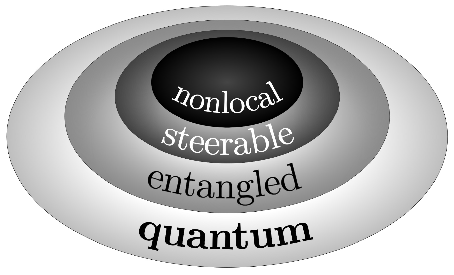
Figure 2.
Illustration of the setup to compute the CHSH correlation function . By separating the systems I and II, one can perform measurements of distinct observables, e.g., and for I at detector 1 and and for II at detector 2. From many realizations of the experiment, leading to distinct outcomes , , , (assuming only the values -1 or +1, two levels systems), one obtains the correlation function (the actual expression in Section 5).
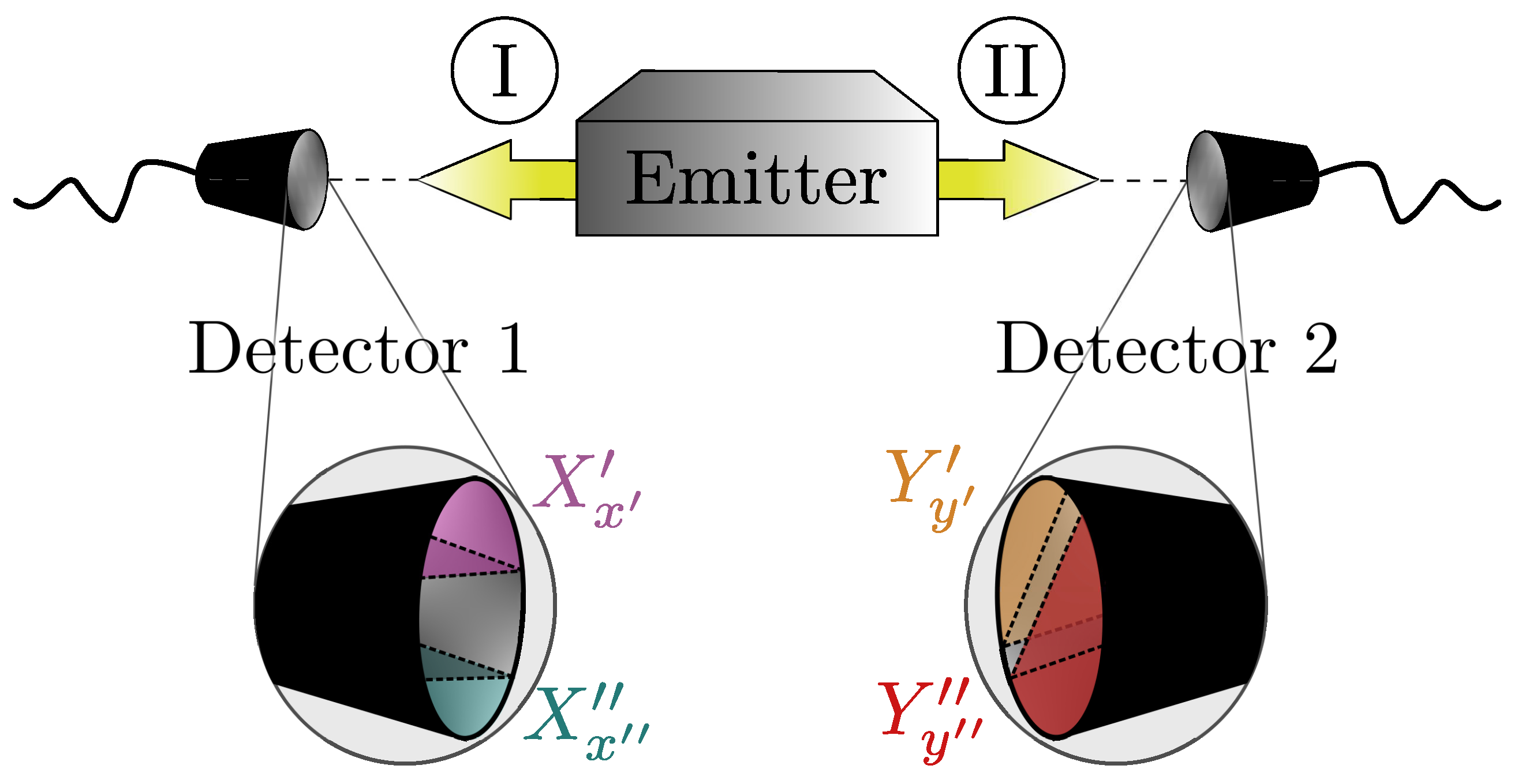
Figure 3.
Schematics of typical processes in forming and measuring an EPR state (constituted by the entanglement of two systems, I and II): the preparation of the entangled state; the spatial separation of its two parts, I and II; and the possible measurements of an observable for system I, allowing to infer (with 100% certainty) an observable for system II.
Disclaimer/Publisher’s Note: The statements, opinions and data contained in all publications are solely those of the individual author(s) and contributor(s) and not of MDPI and/or the editor(s). MDPI and/or the editor(s) disclaim responsibility for any injury to people or property resulting from any ideas, methods, instructions or products referred to in the content. |
© 2023 by the authors. Licensee MDPI, Basel, Switzerland. This article is an open access article distributed under the terms and conditions of the Creative Commons Attribution (CC BY) license (http://creativecommons.org/licenses/by/4.0/).
Copyright: This open access article is published under a Creative Commons CC BY 4.0 license, which permit the free download, distribution, and reuse, provided that the author and preprint are cited in any reuse.


