Submitted:
05 July 2023
Posted:
06 July 2023
You are already at the latest version
Abstract
Navigation is the most challenging issue in autonomous vehicles. Researchers in the current era have developed many Artificial Intelligence techniques to navigate, generate paths, and avoid obstacles for optimum path planning for autonomous vehicles. Different studies have investigated bio-inspired techniques to overcome the navigation issue, including obstacle avoidance. This paper uses new meta-heuristic optimization techniques called Dragonfly Algorithm (DA) to set the goal by detecting and avoiding obstacles with minimum human interference. For effective results, the Dragonfly-Fuzzy hybrid algorithm is analyzed over the unstructured environment because individual techniques may not be sure of an optimal solution over all configurations. The main advantage of the proposed hybrid controller is that it combines the multiple features of different approaches into a single controller. This paper compares simulation and experimental findings over various environmental conditions to the individual algorithm. Regarding time and path optimization, the hybrid Dragonfly-Fuzzy controller performs better than the respective controller.
Keywords:
autonomous vehicle
; path planning
; hybrid controller
; dragonfly algorithm
; fuzzy logic
1. Introduction
The fast development of the logistics industry creates the demand for intelligent autonomous vehicles for efficient and fast processes [1]. Autonomous vehicles replacing human labour in labour-intensive, repetitive, and dangerous areas have received considerable attention, crucial to the operational efficiency and resource consumption of modern factories and warehouses [2]. An autonomous vehicle is an intelligent vehicle that can perceive its environment, gather and analyze important information from its sensor, and identify its current position. This vehicle also generates a feasible path from the initial location to the target location with the decision control to achieve the path through a planned trajectory [3]. Path planning methods is one of the fundamental methods for realizing autonomous vehicle intelligence, which refers to determining an optimum or suboptimal path from the initial location to the target location in a complicated spatial environment based on the initial and target positions provided during vehicle operation [4]. The path planning problems are divided into different static and dynamic environments [5] and refer to different static and dynamic obstacle avoidance [6].
Path planning algorithms have been widely employed for outdoor and interior path planning. Classical approaches, heuristic methods and bioinspired algorithms are typical navigation and motion planning approaches for autonomous vehicle technologies in the context of pathfinding algorithms. Many researchers have implemented various Swarm Intelligence meta-heuristics algorithms inspired by the natural behaviours of some animals (such as grey wolves, ants, and so on) in their quest for survival. Swarm intelligence is used to solve nonlinear problems with real-world implementations using the most advanced science and engineering areas, such as data mining and neural networks. Different swarm intelligent algorithms are utilized for path optimization. For addressing the navigational strategies in autonomous vehicles, Ant Colony Optimization (ACO) [7], Particle Swarm Optimisation (PSO) [8], Firefly Algorithm (FA) [9], Fruit Fly Algorithm (FFA) [10], Bat Algorithm [11], Grey Wolf Optimizer [12], Grasshopper Optimization Algorithm (GOA) [13] and many other algorithms have been utilized for solving different navigational problems of autonomous vehicles.
Various research has been performed on multi-objective-based path planning since it is required to evaluate numerous elements concurrently, such as travel distance, collision safety, and path flexibility, rather than simply generating a path considering only one component. Hybridization techniques, in which bioinspired algorithms are mixed with heuristic algorithms like A* [14] and Fuzzy logic [15], can improve the efficiency of autonomous vehicles. When compared to separate controllers, this A*-Fuzzy hybrid approach optimizes the shortest path while also avoiding obstacles [16]. Another intelligent hybrid approach called Quarter Orbits Particle Swarm Optimization (QOPSO) secures the optimal path and improves the final path, free from a collision [17]. On the other hand, when Quarter Orbit is considered alone, it consumes more power and has an unsmooth path.
This paper uses a traditional, bioinspired, and hybrid technique to find the shortest collision-free path. This proposed work for an unstructured environment delivers a path-planning approach with obstacle avoidance using Fuzzy Logic and Dragonfly Algorithm. This paper demonstrates autonomous vehicle path planning and obstacle avoidance utilizing individual and hybrid controllers. This paper presents a new Dragonfly-Fuzzy hybrid strategy for path finding of autonomous vehicles in static and dynamic environments to optimize the path length and calculate the time when compared to the standalone algorithm.
2. Path Planning algorithms
The key issue in moving the autonomous vehicle from one position to another was identifying the best or close to best desired path by avoiding obstacles in order to reach the target with desirable accuracy. Hence the most crucial function of any navigational technique is safe path planning (by identifying and avoiding obstacles) from the initial place to the target position. As a result, when working in a simple or complex environment, the proper selection of the navigational strategy is the most critical phase in the course planning of an autonomous vehicle. This paper uses Fuzzy Logic and Dragonfly algorithms for path planning and autonomous mobile robot obstacle detection.
2.1. Dragonfly Algorithm
Seyedali Mirjalili proposed the Dragonfly Algorithm [18] in 2015 to solve multi-objective optimization challenges. Static and dynamic swarming behaviours inspire the Dragonfly Algorithm (DA). These two swarming tendencies are very comparable to the two major phases of meta-heuristic optimization: exploration and exploitation. Static swarming, also known as hunting, creates a small group of dragonflies that swiftly adjust their steps in search of food. A dynamic swarm, also known as a migratory swarm, is a huge group of dragonflies travelling long distances for migration. As proposed by Reynolds in 1987, dragonfly swarming behaviours adhere to the concepts of separation, alignment, cohesion, attraction to food, and distraction from opponents. The Dragonfly Algorithm, two primary phases of optimization methods, exploration and utilization, are designed by social interaction in navigation, hunting for food, and fighting compiled enemies dynamically that use the Binary Dragonfly Algorithm (BDA), Multi-objective Dragonfly Algorithm (MODA) and Single–Objective Dragonfly Algorithm (SODA).
The Dragonfly algorithm works on the five basic rules. Where represents the position of the current individual flies, represents the position of neighboring flies and be the number of neighboring individuals.
1. Separation () represents the internal collision avoidance with other flies in the neighborhood, mathematically represented as shown in the Equation (1).
2. Alignment () indicates the matching of the velocity individually between the other neighborhood individuals of the same group; it is mathematically represented as shown in the Equation (2).
here represents the velocity of the ith individuals
3. Cohesion represents the tendency of individuals towards the centre of the mass of the neighborhood; it represents as shown in the Equation (3).
4. Attraction represent the food of the source , which is mathematically represented as shown in the Equation (4).
Where represent the food source of the jth individuals and represent the position of the food source.
5. Distraction represents the distraction from the enemy as shown in Equation (5).
Where represent the position of the enemy of the individuals and represent the enemy position.
If the DA updates the position in the search space, two vectors Step Vector (SV) and Position Vector (PV), are used. The SV can be uploaded using a similar equation used in the PSO algorithm [19]. The Equation (6) will be used for calculating the position vector.
Where denotes the current iteration denoted as the next position , represents the current position denotes the step vector which is represented by Equation (7),
Where denotes the current step vectors; represent the seperation, represents the alignment, represents the cohesion, represents the food source, and represent the distraction, while represents the inertia weight.
If sometimes the dragonfly algorithms have no neighbours, then the dragonfly must do some random movement. In this situation, the position must be updated using Levy’s flight which is represented by the Equation (8)
The main objective of using DA is to navigate the autonomous vehicle into an unstructured environment consisting of different obstacles. This objective is transformed into a minimization problem with two functions. The first is to avoid obstacles, and the second is to find the shortest possible path. Figure 1 depicts the environment of the autonomous vehicle target and goal positions.
2.2. Fuzzy Logic Concept
Lotfi Zadeh invented the concept or origin of fuzzy logic approaches in 1965 [20], and its mechanism is based on human decisions such as yes or no or if-else. The fuzzy logic concept of the numerous dilemma factors provides a meaningful choice representation via its if-else, rule-based mechanism. Its operation is based on misleading and randomly distributed partial data for multiple issues. Unlike linear logic, fuzzy logic models complicated data problems with the most uncertainty. The basic fuzzy logic working model is illustrated in Figure 4.
The basic parameters of the fuzzy logic are given as follows:
- Fuzzification: It is represented as a membership function that defines the input variables.
- Inference and Aggregation: Its parameter shows the final output of the fuzzy rules.
- Defuzzification: Its Crisp value converted from fuzzy-based output will be found.
The concept of fuzzy inference Basic mapping techniques uses input data with output variables. In fuzzy inference, the if-then rule is used. It is also the foundation for its decision-making. Let the different objects(x) denoted by and x be the known pair for fuzzy set A.
From the Equation (9), defines the fuzzy membership function provided for set A. In other, the membership values used to measure x will be 0 to 1. The basic fuzzy logic problem is solved by two types of function, i.e., trapezoidal and triangular. The Equation (10) describes the triangular membership function.
To explain the principle of maxima and minima, the given Equation (10) can represent by the Equation (11),
Similarly, the given trapezoidal function can be explained by using the four parameters , as represented in the Equation (12) given below,
In above equation determines the values of the x-coordinates (with ) of the corners of the defuzzification-trapezoidal membership function.
Defuzzification is mathematically explained in the subsequent equation, which employs the centre of gravity principle to turn the fuzzy set into a crisp value.
Where define the crisp output value and represents the centre of the membership function. While and reflects the area under the membership function.
Research manuscripts reporting large datasets that are deposited in a publicly available database should specify where the data have been deposited and provide the relevant accession numbers. If the accession numbers have not yet been obtained at the time of submission, please state that they will be provided during review. They must be provided prior to publication.
Interventionary studies involving animals or humans, and other studies that require ethical approval, must list the authority that provided approval and the corresponding ethical approval code.
3. DRAGONFLY-FUZZY HYBRID CONTROLLER
The proposed hybrid controller was modelled by considering the vehicle-to-obstacle distance, vehicle-to-goal distance and the mutual distance between the vehicle and its motion. This controller filters all navigation parameters to give the required angle for an autonomous vehicle. Dragonfly controller will be placed first in the hybrid controller, which gets the input as Front Obstacle Distance (FOD), Left Obstacle Distance (LOD) and Right Obstacle Distance (ROD), whereas the output will be the Steep Heading Angle (SHA). The output of the DA controller and the vehicle’s current position ( FOD, LOD, ROD) will be the input of the fuzzy logic controller. Figure 5 shows the hybrid controller architecture.
To calculate the key pointers (FOD, LOD, ROD), the autonomous vehicle used in this study is equipped with eight sensors around its periphery to detect the obstacle and position of the goal. The hybrid controller considers the DA controller’s input and distance from the obstacles to providing the SHA. This finding from the DA controller is used to train the fuzzy logic controller to get the Total Heading Angle (THA) for all environmental conditions.
The obstacle avoidance feature is built to maintain the vehicle from colliding with the obstacles in the environment. The food source should be kept as far away from the nearest obstacle as possible (global best position). The source of food should be kept as far away from the nearest obstacle as possible (global best position). The Euclidean distance between the global best position ( food Source) and the most immediate environmental obstacle is used to calculate the objective function given by the Equation (14),
Where and are the best position while and is the closest obstacle position. The Euclidean distance between the most relative obstacle and the vehicle is calculated using the Equation (15),
The best position for the Dragongly food source should be as close to the goal as possible. The target-seeking objective function is defined as the Euclidean distance between the best position and the goal in the environment is given by the Equation (16),
Where and are the goal position and is the minimum Euclidean distance from the vehicle to the source position of food.
The equation defines the objective function of path optimization, which combines obstacle-seeking and target-seeking behaviour.
When the vehicle moves in an unstructured environment, encounter different obstacle known as. In this objective function, it is clearly specified that when comes closer to the goal, it decreases, resulting moves far away from the obstacles. C1 and C2 in the objective function are known as fitting/controlling parameters, and it is evident that these parameters have a direct influence on the vehicle trajectory. If C1 is too large, the robot will be far away from the obstacles; if C1 is too tiny, the robot may crash with an object in the surroundings. Similarly, if C2 is big, the robot is more likely to take a short/optimal approach to the target, but small values result in longer pathways. These control settings will result in faster convergence of the objective function and removal of local minima. The control settings in this work are chosen using trial and error approaches.
Fuzzy logic is the universal approximator capable of performing any nonlinear mapping between sensor data input and central variable output. Terms used for FOD, LOD, and ROD are “much closer”, “very closer”, “closer”, “away”, “very away”, and “much away”. The heading angle uses the terms “wider wide”, “moderately wide”, “wide”, “short”, “moderately short”, and “too short” as output. The membership functions used are shown in Figure 6. All the Fuzzy if-then rule mechanisms are illustrated in the Table 1 and Table 2.
4. EXPERIMENTAL AND SIMULATION RESULTS
The simulation and experimental results are provided here to validate the proposed experimental controller. The FIREBIRD V robot is used in this experiment, as shown in Figure 7. Fire Bird V supports ATMEGA2560 (AVR) microcontroller adaptor board, making it very versatile.
An environment with obstacles was tested on the simulation software MATLAB to determine the optimality of the proposed DFA-based controller in terms of path length and time required for navigation. Three controllers (DA, FL, DA-FL) were used for navigation, and the output is illustrated in Figure 8, Figure 9 and Figure 10. The Path length and time of the three controllers are shown in Table 3.
All three controllers (DA, FL, DA-FL) are experimentally run in a similar environment to validate the simulation results, as shown in Figure 11, Figure 12 and Figure 13. These results are presented over its path length and navigation time, as shown in Table 4
The proposed Dragongly-Fuzzy hybrid controller is compared to existing standalone navigational controllers in the same environmental configuration shown in Figure 14 to determine its success. Table 5 and Table 6 compares the simulation and experimental results for all three controllers in terms of time and path length.
5. Conclusion
Different standalone metaheuristic algorithms were investigated in this proposed work to solve the navigational problem of an autonomous vehicle, and a new hybrid method was introduced. The proposed DA-FL controller is tested successfully over the standalone DA and FL controllers in a static obstacle environment. A set of experiments are performed to adjust the autonomous vehicle's parameters, which are directly connected to the smoothness of the generated path. The suggested technique allows the autonomous vehicle to reach its destination while avoiding obstacles and following a much-optimized path. Experimental and simulation findings demonstrate that the variation percentage is around 4% to 5% with the optimum path and time. When comparing the proposed hybrid controller and the standalone controller, it was found that the DA-FL hybrid controller takes the shortest path and time. In the future, the Dragonfly-Fuzzy controller can be implemented in a dynamic environment. It can be tested for navigation for underwater robots and aerial vehicles.
Author Contributions
Conceptualization and Supervision, B.P. and S.B.; methodology and Validation, B.P.; software and investigation, V.D.; writing—original draft preparation, B.P and V.D.
Funding
This research received no external funding.
Acknowledgments
The support from the UAV and Robotics Laboratory of the School of Engineering and IT, MATS University, was appreciated.
Conflicts of Interest
The authors declare no conflict of interest.
References
- F. Oleari, M. Magnani, D. Ronzoni, and L. Sabattini, "Industrial AGVs: Toward a pervasive diffusion in modern factory warehouses," in 2014 IEEE 10th International Conference on Intelligent Computer Communication and Processing (ICCP), 2014: IEEE, pp. 233-238.
- J. Monios and R. Bergqvist, "Logistics and the networked society: A conceptual framework for smart network business models using electric autonomous vehicles (EAVs)," Technological Forecasting and Social Change, vol. 151, p. 119824, 2020. [CrossRef]
- D. Nakhaeinia, S. H. Tang, S. M. Noor, and O. Motlagh, "A review of control architectures for autonomous navigation of mobile robots," International Journal of the Physical Sciences, vol. 6, no. 2, pp. 169-174, 2011.
- P. Sudhakara, V. Ganapathy, B. Priyadharshini, and K. Sundaran, "Obstacle avoidance and navigation planning of a wheeled mobile robot using amended artificial potential field method," Procedia computer science, vol. 133, pp. 998-1004, 2018. [CrossRef]
- Yazici, G. Kirlik, O. Parlaktuna, and A. Sipahioglu, "A dynamic path planning approach for multirobot sensor-based coverage considering energy constraints," IEEE transactions on cybernetics, vol. 44, no. 3, pp. 305-314, 2013.
- B. Patle, B. Patel, and A. Jha, "Rule-Based Fuzzy Decision Path Planning Approach for Mobile Robot," in 2018 Fourth International Conference on Computing Communication Control and Automation (ICCUBEA), 2018: IEEE, pp. 1-7.
- V. Ganapathy, P. Sudhakara, T. J. Jie, and S. Parasuraman, "Mobile robot navigation using amended ant colony optimization algorithm," Indian Journal of Science and Technology, vol. 9, no. 45, pp. 1-10, 2016. [CrossRef]
- J. Xin, S. Li, J. Sheng, Y. Zhang, and Y. Cui, "Application of improved particle swarm optimization for navigation of unmanned surface vehicles," Sensors, vol. 19, no. 14, p. 3096, 2019. [CrossRef]
- Patel and B. Patle, "Analysis of firefly–fuzzy hybrid algorithm for navigation of quad-rotor unmanned aerial vehicle," Inventions, vol. 5, no. 3, p. 48, 2020. [CrossRef]
- B. Xing, W.-J. Gao, B. Xing, and W.-J. Gao, "Fruit fly optimization algorithm," Innovative Computational Intelligence: A Rough Guide to 134 Clever Algorithms, pp. 167-170, 2014. [CrossRef]
- G.-G. Wang, H. E. Chu, and S. Mirjalili, "Three-dimensional path planning for UCAV using an improved bat algorithm," Aerospace Science and Technology, vol. 49, pp. 231-238, 2016. [CrossRef]
- J. Liu, X. Wei, and H. Huang, "An improved grey wolf optimization algorithm and its application in path planning," IEEE Access, vol. 9, pp. 121944-121956, 2021. [CrossRef]
- Y. Meraihi, A. B. Gabis, S. Mirjalili, and A. Ramdane-Cherif, "Grasshopper optimization algorithm: theory, variants, and applications," Ieee Access, vol. 9, pp. 50001-50024, 2021.
- K. Guruji, H. Agarwal, and D. Parsediya, "Time-efficient A* algorithm for robot path planning," Procedia Technology, vol. 23, pp. 144-149, 2016. [CrossRef]
- G. Antonelli, S. Chiaverini, and G. Fusco, "A fuzzy-logic-based approach for mobile robot path tracking," IEEE transactions on fuzzy systems, vol. 15, no. 2, pp. 211-221, 2007. [CrossRef]
- V. Dubey, S. Barde, and B. Patel, "Obstacle Finding and Path Planning of Unmanned Vehicle by Hybrid Techniques," in Information Systems and Management Science: Conference Proceedings of 4th International Conference on Information Systems and Management Science (ISMS) 2021, 2022: Springer, pp. 28-36.
- Z. E. Kanoon, A. Araji, and M. N. Abdullah, "Enhancement of Cell Decomposition Path-Planning Algorithm for Autonomous Mobile Robot Based on an Intelligent Hybrid Optimization Method," International Journal of Intelligent Engineering and Systems, vol. 15, no. 3, pp. 161-175, 2022.
- S. Mirjalili, "Dragonfly algorithm: a new meta-heuristic optimization technique for solving single-objective, discrete, and multi-objective problems," Neural computing and applications, vol. 27, pp. 1053-1073, 2016.
- J. Kennedy and R. Eberhart, "Particle swarm optimization," in Proceedings of ICNN'95-international conference on neural networks, 1995, vol. 4: IEEE, pp. 1942-1948.
- L. A. Zadeh, "Fuzzy sets," Information and control, vol. 8, no. 3, pp. 338-353, 1965.
Figure 1.
Autonomous vehicle positioning in the presence of an obstacle.
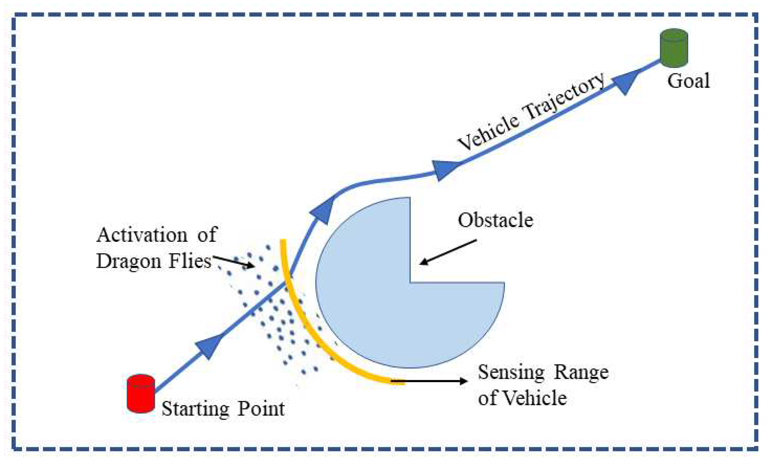
Figure 2.
Dragonfly Algorithm architecture.
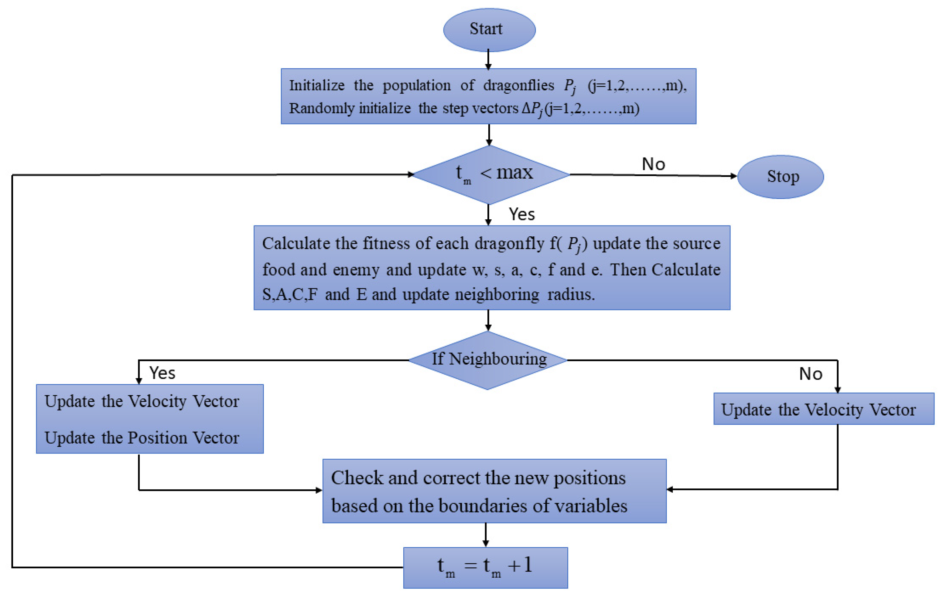
Figure 3.
Pseudo-code of Dragonfly Algorithm.

Figure 4.
Schematic diagram of fuzzy logic.
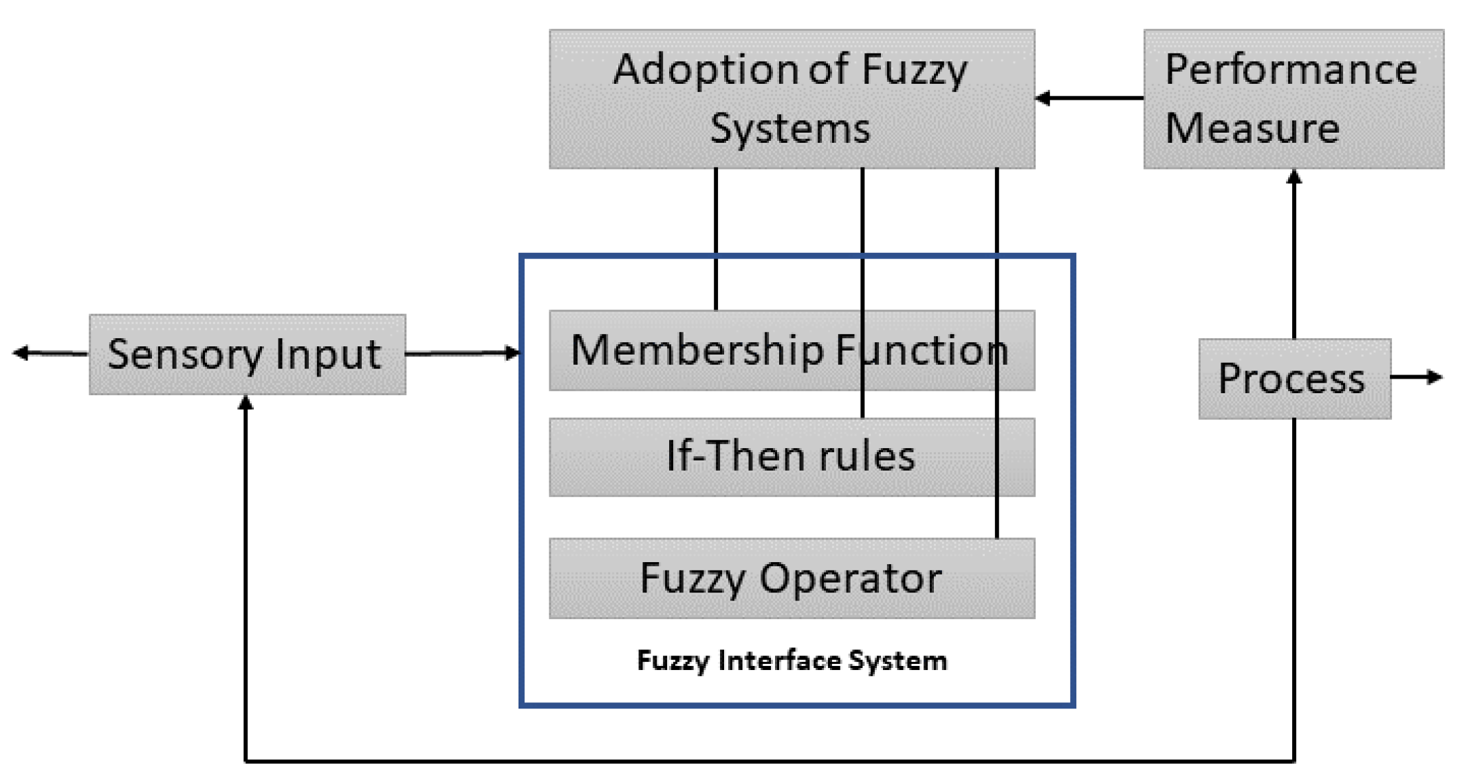
Figure 5.
Dragonfly-Fuzzy hybrid controller architecture.
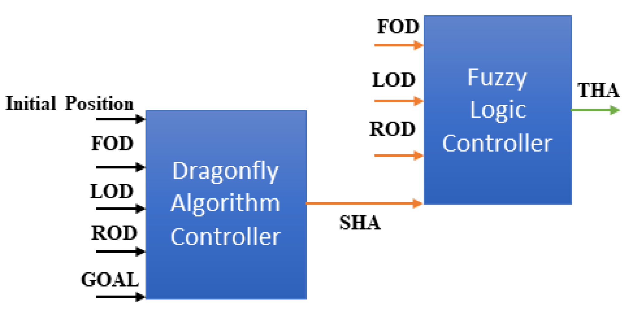
Figure 6.
Fuzzy Logic membership function (a) Trangular (b) Trapezoidal (v) Gaussian.
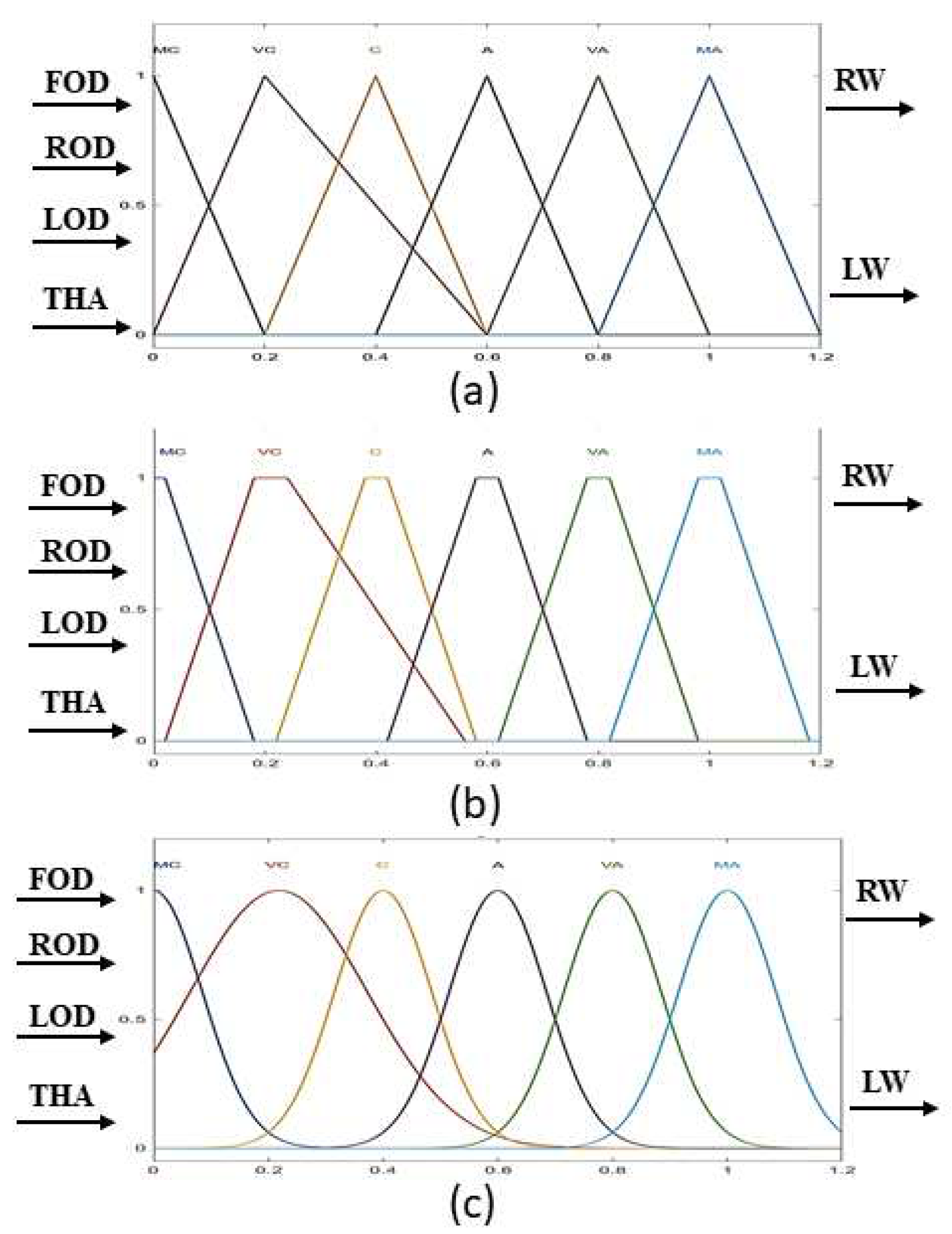
Figure 7.
Firebird V robot.
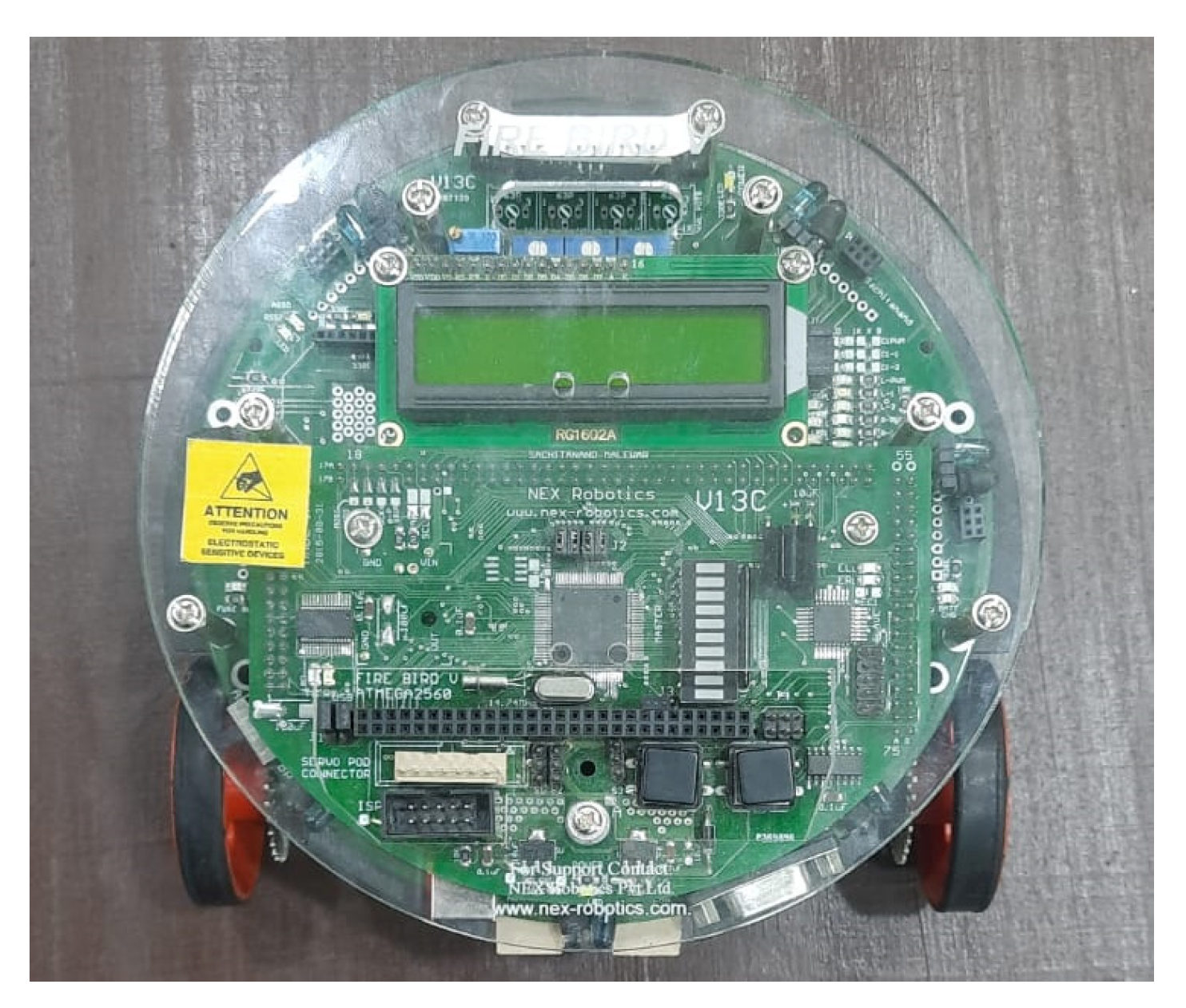
Figure 8.
Navigation using DA standalone.
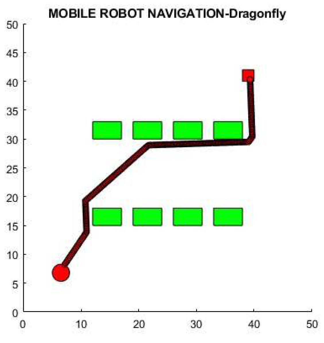
Figure 9.
Navigation using FL standalone.
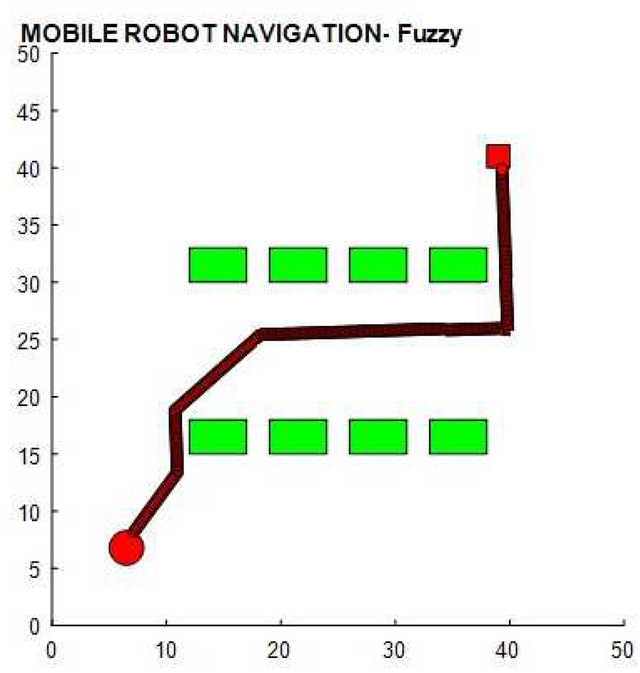
Figure 10.
Navigation using DA-FL hybrid.
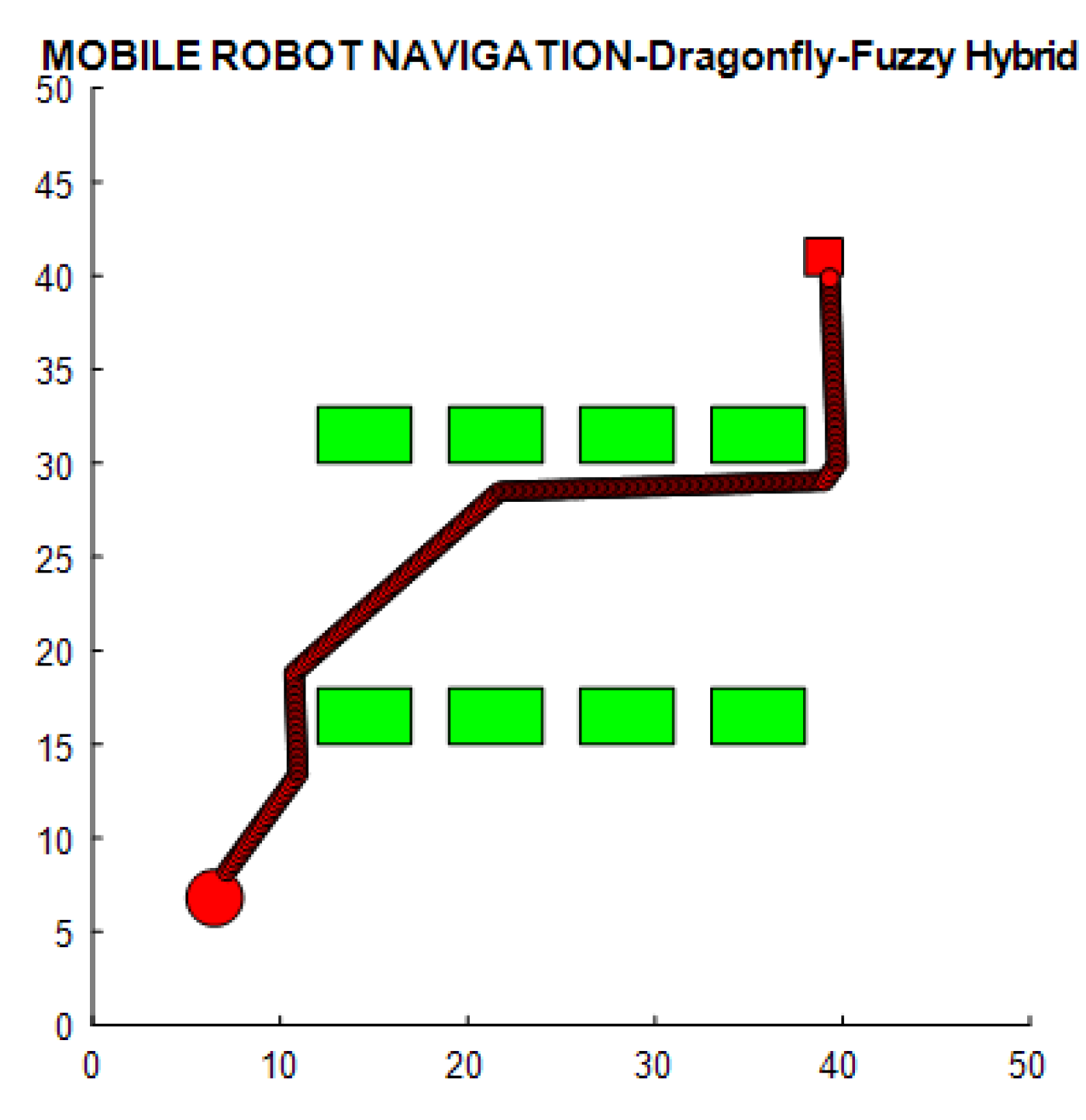
Figure 11.
Navigation using DA standalone.
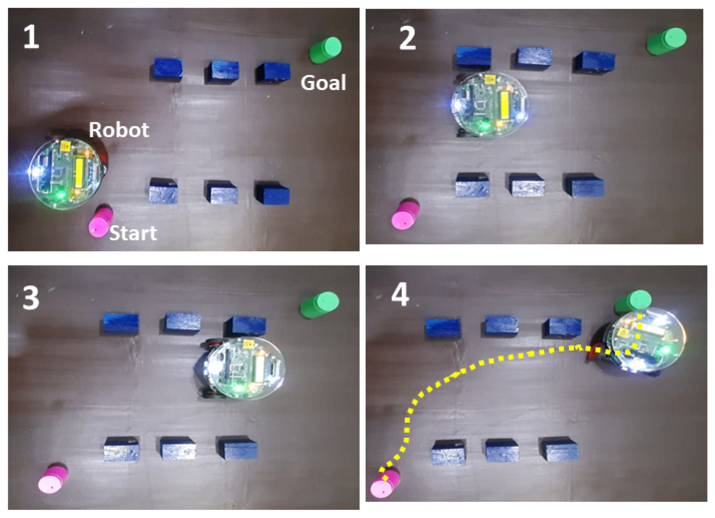
Figure 12.
Navigation using FL standalone.
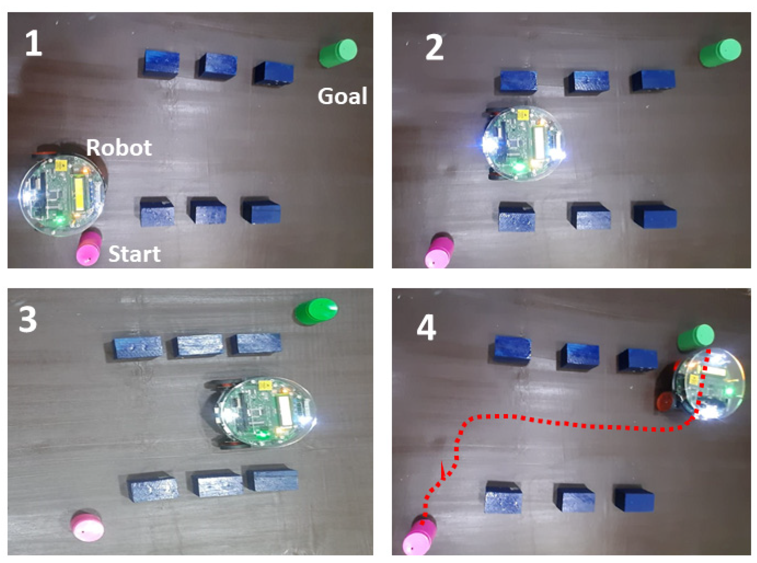
Figure 13.
Navigation using DA-FL hybrid.
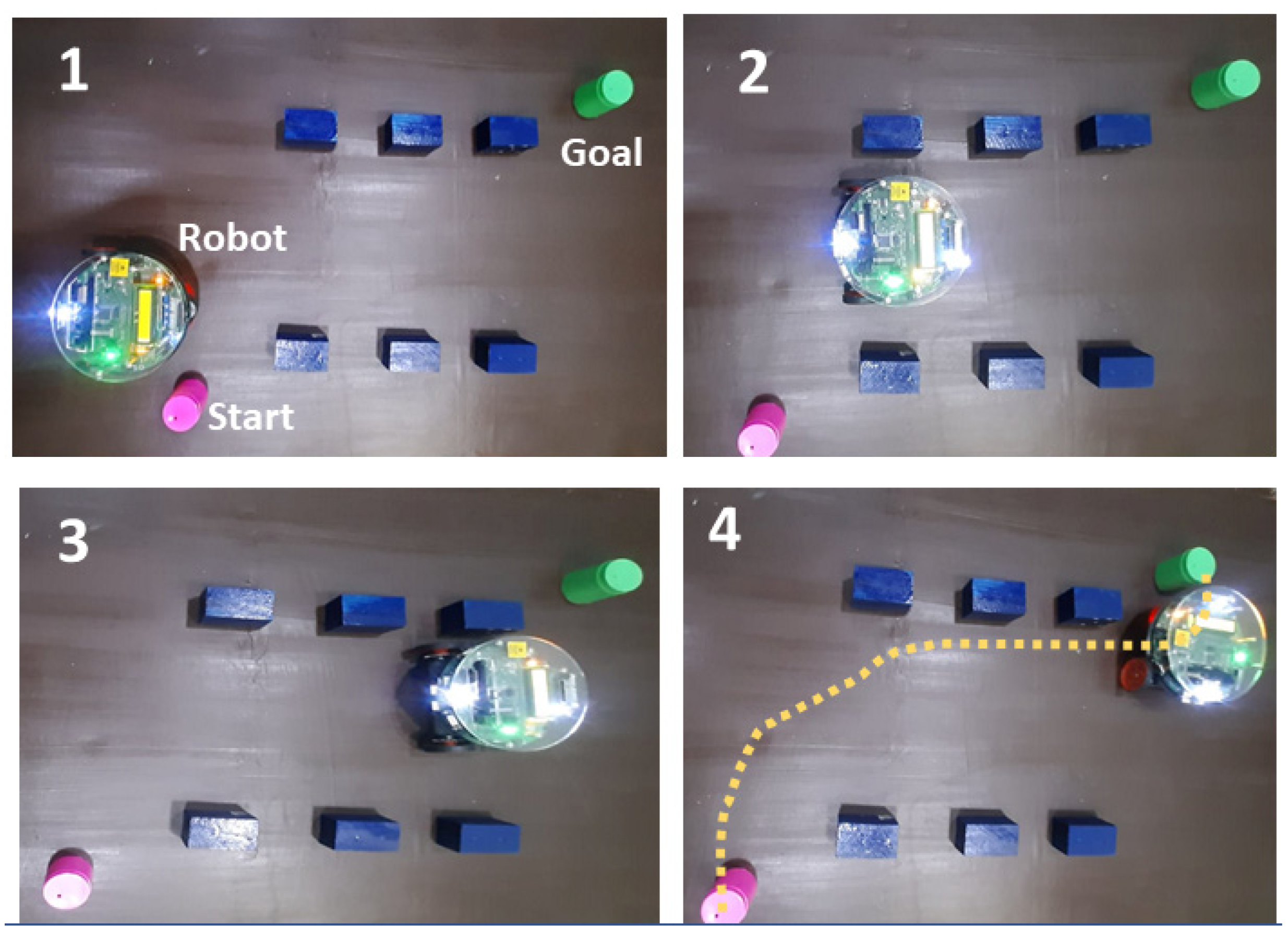
Figure 14.
DA-FL hybrid controller versus another controller.
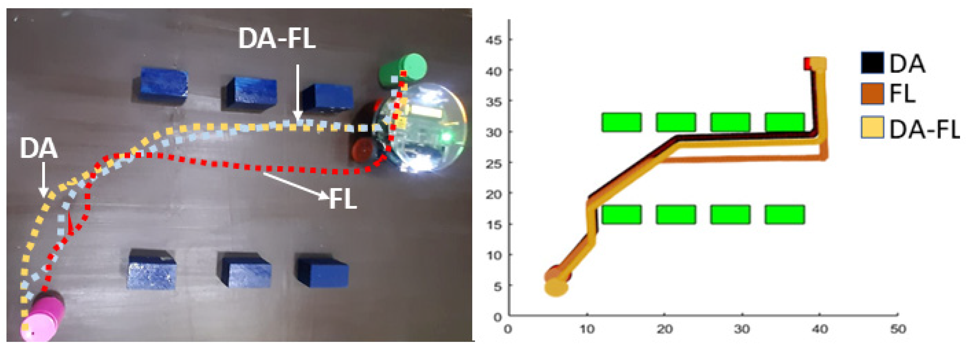

Table 1.
FL parameters for obstacles.
| Linguistic Variable | MN | VC | C | A | VA | MA |
|---|---|---|---|---|---|---|
| LOD | 0.0 | 0.2 | 0.4 | 0.6 | 0.8 | 1.0 |
| ROD | 0.2 | 0.4 | 0.6 | 0.8 | 1.0 | 1.2 |
| FOD | 0.4 | 0.6 | 0.8 | 1.0 | 1.2 | 0.0 |
Table 2.
FL parameters of heading angle.
| Linguistic Variable | WW | MW | W | S | MS | TS |
|---|---|---|---|---|---|---|
| THA | -180 | -120 | -60 | -10 | 10 | 60 |
| -120 | -60 | -30 | 0 | 60 | 120 | |
| -60 | -30 | 0 | 10 | 120 | 180 |
Table 3.
Simulation path length and time of DA, FL, DA-FL.
| S.No | Controller | Simulation Path Length (‘cm’) | Simulation Path Time (‘cm’) |
| 1 | Dragonfly | 120.4 | 11.8 |
| 2 | Fuzzy logic | 169.8 | 13.2 |
| 3 | DA-FL hybrid | 113.0 | 10.9 |
Table 4.
Experimental path length and time of DA, FL, DA-FL.
| S.No | Controller | Experimental Path Length (‘cm’) | Experimental Path Time (‘sec’) |
| 1 | Dragonfly | 126.22 | 12.6 |
| 2 | Fuzzy logic | 136.68 | 14 |
| 3 | DA-FL hybrid | 118.66 | 11.5 |
Table 5.
Path length comparison of DA, FL, DA-FL.
| Controller | Experimental Path Length (‘cm’) | Simulation Path Length (‘cm’) | % Error |
| Dragonfly | 126.3 | 120.4 | 4.58 |
| Fuzzy logic | 136.7 | 169.8 | 5.10 |
| DA-FL hybrid | 118.6 | 113.0 | 4.40 |
Table 6.
Navigational time comparison of DA, FL, DA-FL.
| Controller | Experimental Path Time (‘Sec’) | Simulation Path Time (‘Sec’) | % Error |
| Dragonfly | 12.6 | 11.8 | 5.80 |
| Fuzzy logic | 14 | 13.2 | 5.76 |
| DA-FL hybrid | 11.5 | 10.9 | 5.20 |
Disclaimer/Publisher’s Note: The statements, opinions and data contained in all publications are solely those of the individual author(s) and contributor(s) and not of MDPI and/or the editor(s). MDPI and/or the editor(s) disclaim responsibility for any injury to people or property resulting from any ideas, methods, instructions or products referred to in the content. |
© 2023 by the authors. Licensee MDPI, Basel, Switzerland. This article is an open access article distributed under the terms and conditions of the Creative Commons Attribution (CC BY) license (http://creativecommons.org/licenses/by/4.0/).
Copyright: This open access article is published under a Creative Commons CC BY 4.0 license, which permit the free download, distribution, and reuse, provided that the author and preprint are cited in any reuse.


