
Submitted:
30 June 2023
Posted:
03 July 2023
You are already at the latest version
Abstract
Efficient natural convection-cooled heat sinks are vital to the future of electronics cooling due to their low energy demand in the absence of an external pumping agency in comparison to other cooling methods. The present study is aimed to identify the most effective fin design for enhancing heat transfer in natural convection applications. Initially, a baseline case with rectangular fins was considered in the present study and it was optimized with respect to fin spacing. This optimized baseline case is then validated against the semi-empirical correlation proposed by Elen-baas (1942) [2]. Upon good agreement, the validated model is used for comparative analysis of different heat sink configurations with rectangular, trapezoidal, curved, and angled fins. The optimised fin spacing obtained for the baseline case is also used for the other heat sink configura-tions and then the fin designs are further optimized for better performance. However, for the an-gled fin case, the optimized configuration proposed by Zhang et al. (2020) [3] is adopted in the present study. This study is carried out with Ansys Fluent for a Rayleigh number of 2.4 × 10^6. The proposed novel curved fin design with a shroud defined as Case C4 showed a 4.1% decrease in the system’s thermal resistance with an increase in the heat transfer coefficient of 4.4% when compared to the optimized baseline fin case. The obtained results are further non-dimensionalized with proposed scaling in terms of the baseline case for the two novel heat sink cases (trapezoidal, curved).
Keywords:
Natural Convection
; Heat Sink
; Plate Fins
; Computational Fluid Dynamics
; Shape Optimization
; Electronics Cooling
1. Introduction
As the world becomes more reliant on digital devices and as the systems become more compact, cooling of electronics has increased importance. Thermal energy produced by electronic components can be devastating to the integrity of devices if not properly dissipated. Passive cooling systems are much advantageous due to their low their low energy demand in the absence of an external pumping sources like blowers, fans etc. [1] as in such flow will be induced by non-uniform density in the fluid [4]. The industry standard for a natural convection-cooled heat sink usually involves a vertically oriented base plate with an evenly-spaced rectangular plate fin array, with or without shroud [5]. The sizing, arrangement, and shape of a heat sink fins affect its thermal performance. A significant amount of research has been conducted into varying both fin parameters and proposing novel designs, all with the aim of improving the system’s overall heat transfer performance. Numerous designs have been proposed in the literature over the past many years, many claiming to achieve significant performance enhancement compared to the rectangular fin baseline case. While some of these designs hold merit, many often compare their results to an unoptimized baseline case which puts into question the validity of their findings.
The simplest heat sink fins are made up of an array of vertical rectangular parallel plates, with many innovative designs generated from variations of this simple setup. The design of these fins can have a large effect on the heat transfer rate, as can the spacing, width, thickness, and height of the fins. Bar-Cohen and Rohsenow [6] found that for a pair of vertical parallel plates there exists an optimum fin spacing for which heat transfer for the system will be maximized. Anbar et al. [7] conducted a comprehensive experimental analysis of rectangular fin heat sinks and found that for a fixed base to ambient temperature, the maximum heat transfer achieved is a function of the fin spacing and length. Bar-Cohen et al. [8] performed a detailed computational analysis on the effect of fin spacing, fin height, fin length and temperature difference on the rate of heat transfer for a fin array. The study was carried out with an isothermal base plate of fixed dimension up on which many fins were attached of thickness () and spacing (). The overall heat transfer coefficient was evaluated for varying values of and . The results showed that at an optimal fin spacing and thickness, the heat transfer coefficient was maximized.
More elaborate fin designs have been proposed in the literature that deviate from the standard rectangular profile. Chen et al. [9] used eight different types of heat sinks and performed optimizations with ten different objective functions on these. The study highlighted the importance of proper selection of optimization objective functions. Ray et al. [10] proposed a variety of designs using various configurations of branched and interrupted fins. Five innovative designs consisting of different permutations of branched and interrupted fins were proposed and analyzed. The study concluded that the fins with interruptions increased heat dissipation compared to the uninterrupted baseline case due to increased fluid mixing. For the branched fins, the overall heat transfer was highest when the secondary fins moved furthest from the baseplate. This is due to the creation of a chimney-like effect which causes an increase in air movement due to a suction effect. Chang et al. [11] proposed a vertical dimpled fin array which showed higher thermal performance than a standard rectangular profiled array. The proposed geometry was created by altering existing rectangular fins with a repeating pattern of different radius dimples. The dimples were concave against the rectangular fin and alternated on each side of the fin, producing a sinusoidal-like side-profile. The study found that the Nusselt number increases with an increase in Rayleigh number. Moreover, a nine-fin dimpled array produced a 61 – 68% higher Nusselt number than a thirteen-fin array for the same Rayleigh number. Joo et al. [12] conducted a comparison between plate and pin fin heat sinks by optimizing the fin spacing for best thermal performance. Using pre-existing correlations for vertical plate heat sinks, a theoretical optimum spacing was calculated for the plate fins. Under the same boundary conditions, the plate fin heat sink performed better by dissipating more heat overall. The pin fin heat sink did however perform significantly better when the objective function was set to heat dissipation per unit mass.
Zhang et al. [3] proposed and tested a novel ‘W-type’ fin array for natural convection heat transfer that was tested experimentally and verified using CFD. The array consists of several angled fins arranged in columns of alternating directions. This novel design was compared against a baseline array of vertical rectangular fins of the same length and on the same sized base plate. The variation of heat transfer was examined for changing fin spacing, fin length, fin angle, fin thickness and Rayleigh number. The observations found that an increase in the heat transfer rate was achieved by increasing the number of fin elements and the angle of inclination of the fin. A comparison between the novel W-type fins and rectangular fin array showed a significant enhancement for the W-type design. Several other studies on angled fin configurations mainly with chevron fins were also carried out [13,14,15] which showed a significant impact of chevron angle on the thermal resistance and heat transfer performance. The observations found in [14] showed that by decreasing the chevron angle, an increase in the total thermal resistance and heat transfer is achieved.
Since there is a lack of agreement as to which heat sink design achieves best heat transfer performance, the present study aims at a comparative analysis of different optimized heat sink configurations with rectangular, trapezoidal, curved, and angled fins. As seen in [3], the W-type fin array-based heat sink containing angled fins arranged in columns of alternating directions performed better than other designs. As a result of this, the present study is focused on proposing an optimized novel fin design for a fixed dimensioned baseplate heat sink on comparative basis. These novel designs take inspiration from the geometries proposed in the recent literature which exhibited a promising performance. The final results are presented in comparison to an optimized rectangular baseline heat sink case to ensure any actual improvement is genuine.
2. Materials and Methods
The present study aims to identify, by means of computational fluid dynamics (CFD) and numerical shape optimization, the most effective fin design for enhancing heat transfer in natural air convection. The target end applications are predominantly in electronics cooling, where the Rayleigh number is generally low enough for the flow to remain laminar. Initially, a baseline case with rectangular fins was considered and it was optimized with respect to fin spacing. This optimized baseline case is used for comparative analysis of different heat sink configurations with rectangular, trapezoidal, curved, and angled fins. The optimized fin spacing obtained for the baseline case is also used for the other heat sink configurations and then the fin designs are further optimized for better performance. However, for the angled fin case, the optimized configuration proposed by Zhang et al. [3] is adopted.
To ensure continuity in the testing, a consistent meshing approach, domain size, and CFD solver setup were used across each of these design cases. Also, for reliable relative comparison between tests, several parameters were fixed across all the cases. Table 1 shows the list of parameters fixed for all the design cases. Each case is optimized by carrying out a parametric design study on their geometry to find the fin shape that minimizes the thermal resistance for that specific heat sink configuration.
2.1. Computational Setup and Boundary Conditions
To decrease the computational time and complexity, only half of a channel width was modelled (i.e., from midway between one fin to midway through the channel). This was achieved using symmetry boundary conditions on the front and back faces of the domain [16] as shown in Figure 1. A pressure inlet boundary condition was used on the bottom and left side faces of the domain, while a pressure outlet boundary condition was used on the top face [17]. A constant heat flux boundary condition was used at the right side (back face of the heat sink) region. Adiabatic and no slip boundary conditions were used for the rest of the back wall. Similar to the findings of [3], a domain height of 3 to 5 times the fin height above the heat sink and 1 to 2 times the fin height below, and a depth of 2 to 5 times the fin length is sufficient to ensure the results are independent of the domain size. Using these values as a reference point, a domain independence study was conducted that resulted in a domain height of 2 below and 3 above, with a domain depth of 2 to the left of the top of the heat sink fins. This equals to an overall height and depth of 600 mm x 300 mm for a fin height mm and fin length mm.
Since this was a natural convection study, a pressure-based solver was chosen given its ability to better handle such conditions. By estimating the Rayleigh number present in this scenario, the flow regime that will occur can be estimated. For a Rayleigh number of less than 1x10⁹ (based on the vertical length of the heated surface), it can be assumed that the resulting flow will be laminar [19]. Using an estimated heat sink temperature difference of 35-60 K and ambient air temperature of 300 K, the Rayleigh number is calculated to vary from . Since this is significantly smaller than , the laminar model is selected and should be sufficient to capture the fluid flow. To verify other scenarios of interest, a model capable of resolving the transition from laminar to turbulent flow was also used. The transition () shear stress transport (SST) model was chosen given its capability of modelling both laminar and turbulent flows [19]. A coupled pressure-velocity scheme was employed to solve the Navier-Stokes equations and energy equation, which governs the fluid flow and heat transfer in the system, respectively. This method was chosen over the SIMPLE scheme since it deals with natural convection scenarios better because it simultaneously solves the governing equations rather than separately, producing a more accurate answer [19].
The list of material properties used in the present study were shown in Table 2. The circulating fluid was chosen to be air whose temperature is initially set to the ambient temperature (300 K). The density variation was approximated by using the Boussinesq approach with a reference value of 1.225 kg/m3 and a thermal expansion coefficient K−1. The heat sink material was chosen to be aluminium alloy 2024 and a heat flux of 4000 W/m2 is applied uniformly to the bottom of the heat sink base. Heat radiation is not modelled.
The geometry used for the simulations contained two domains: the heat sink as solid Al-2024 and air as the fluid domain. The fluid domain was meshed using tetrahedrons while the solid domain was meshed with hexahedrons. A mesh convergence study was carried out to (i) verify solution independence and (ii) obtain a sufficiently fine mesh that would provide accurate results without excessively high computational cost, thus facilitating numerical optimization. The number of mesh elements was varied mainly using the global element size as an input parameter. The mesh convergence was assessed by measuring the average heat source temperature across varying mesh density, the results of which can be seen in Figure 2.
The temperature converged at approximately 334.48 K after the mesh was refined. A mesh element size of 0.0018 m (approx. 500,000 elements) was chosen as sufficiently fine to produce accurate results. This mesh sizing was kept consistent throughout the testing of the baseline case. However, when the subsequent cases are needed to be analyzed by using a turbulence model, then the mesh had to undergo further refinements. For the Transition-SST turbulence model, the value of y+ in the wall-adjacent cell layers needs to be less than or equal to 1 to provide accurate results [19]. To do so, the inflation layers were adjusted for each case in which the turbulence model was used and the maximum y+ value for such cases was ensured to be below 1.
2.2. Design Cases
Table 3 shows the summary of the heat sink cases adopted in the present study. Each of the design case can be identified with a specific design code starting from A1 to D2. Four different heat sink configurations with (A) rectangular, (B) trapezoidal, (C) curved, and (D) angled fins were examined. For the novel cases of trapezoidal and curved heat sink configurations, a shroud located at the end of the fins was considered. However, for the angled fin case, the optimized configuration without shroud as proposed by Zhang et al. [3] is tested and compared with the others. A schematic representation of all the design cases used in the present study are shown in Figure 3. Certain repeating cases (A2, C5, D2, D3 and D4) on the basis of variation in their fin length and spacing are not included in Figure 3.
2.2.1. Rectangular Fin (Case A)
Figure 3 shows the schematic of rectangular baseline fin design with code A1. Before any novel design ideas could be implemented, a set of baseline results has to be established with a rectangular profiled fin. As already established by Bar-Cohen and Rohsenow [6], there exists an optimal spacing for an array of vertical plate fins that can minimize the thermal resistance of a heat sink with a fixed base area. As the spacing increases between each fin, the number of fins that can fit on the fixed base plate decreases. To ensure a more consistent comparison between spacings, only fin spacings that correlated to a whole number of fins fitting on the fixed base plate were considered. To find this spacing the geometry was initially set to have a channel width of 4mm, which corresponded to 25 fins fit onto the baseplate and were increased until the fin spacing of 50 mm was achieved, corresponding to 2 fins on the baseplate. With the spacing set to the new-found optimal value, the fin length was incrementally varied from 30 mm to 200 mm. The size of the domain was configured to adjust to the varying fin length to provide a sufficiently accurate domain size.
2.2.2. Trapezoidal Fin (Case B)
Figure 3 shows the schematic of trapezoidal fin designs with codes B1 and B2. Once a suitably optimized baseline has been established, testing could begin on novel designs. This innovative design featured the inclusion of a planar shroud at the end of the fin length. This shroud serves to add more surface area to the array and acts as a boundary to force the air to flow upwards. These new fin profiles had the same base depth, width, and fin thickness but differing fin upper and lower length. The fin’s midpoint length was fixed at 100 mm while the bottom length of the fin (fin lower length) as shown in Figure.4 (a) was controlled by a design parameter, where the length of the top profile (fin upper length) would change accordingly to create the trapezoidal shape. By configuring the geometry in this way, many permutations could be generated by only varying one design parameter, thus making it far simpler to find an optimal value. When the lower length was set to 100 mm, a rectangular fin profile was generated. This fin was identical to the baseline but included the 1 mm shroud at its end. For a lower length less than 100 mm, a diverging fin was created, while a bottom length greater than 100 mm results in a converging fin shape. Using an identical simulation setup, domain size, and mesh as used for optimizing the baseline heat sink, a natural convection study was conducted for this novel design. The bottom parameter varied from 150 mm to 50 mm in 10 mm increments. The trapezoidal design was also tested for a midpoint of 50 mm in an equivalent manner to assess whether the behavior present was consistent for a different fin length (Case B2).
2.2.3. Curved Fin (Case C)
Figure 3 shows the schematic of curved fin designs with codes C1 to C4. Similar to the trapezoidal fin design case, a new model was created here featuring a shroud attached to the ends of each fin, following a curved spline. This spline is equation driven and connected with two vertex points at its ends. While each end was fixed, the spline’s midpoint is controlled in x-y position as shown in Figure 4(b). Using this new curved fin model, several different parameters were individually varied across various design cases. First, the horizontal position of the spline’s midpoint was varied from 50 mm to 150 mm while its vertical position was fixed at 50 mm (Case C1). Second, the vertical position of it was varied from 20 mm to 80 mm while the horizontal position of the spline was fixed at 50 mm from the base plate (Case C2). Third, the bottom fin length was also kept constant at 100 mm, and the upper profile’s length was varied, creating a variety of hyperbola-like curves while the splines x and y position were both fixed at 50 mm (Case C3). Since these fin shapes would suffer from an increased thermal resistance as the area of the fin was decreased, the heat transfer coefficient was used as the parameter to be maximized. With a local optimal fin shape from Case C3, variation of the overall fin length was conducted to investigate the presence of an optimal fin length that maximized the benefits of the novel curved shape (Case C4). To accurately compare the curved fins to rectangular fins, the lengths of the curved fins were chosen so that their area would be equal to a corresponding length rectangular fin. The fins could then be compared fairly to one another based off equal area rather than one being disadvantaged with a lower surface area to transfer heat through. With a newfound optimal shape, testing on whether the optimal fin spacing from the rectangular fin was still applicable to this innovative design (Case C5). Using the same methodology as for Design Case A1, the fin spacing was varied for an increasing fin spacing that corresponded to a whole number of fins per the size of the base plate. The curved fin was set to the dimensions that corresponded to a fin area equal to the 100 mm rectangular baseline so comparison of the spacings would be as accurate as possible.
2.2.4. Angled Fin (Case D)
Figure 3 shows the schematic of angled fin design with code D1. Angled fins can result in a W-type configuration as shown in Figure 5 from Zhang et al. [3]. The design code D2 configuration is similar to D1 but has a different boundary condition, as shown in Figure 6. For valid comparison, all the design cases in the present study were tested for the same boundary conditions. The fin design in [3] covers a 200 mm wide base plate with four vertical columns of angled fins, which works out to be one column per 50 mm base plate width. To conform to the fixed 100 mm width in the present study, only a 2-column section was used. Figure 5 shows the domain adopted in the present study for the angled fin cases.
Zhang et al. [3] examined several parameters and their effect on the heat transfer performance of the overall system. Rather than conducting our own variation of these parameters, the optimal values proposed in [3] were chosen and used for the present design cases of angled fins. The base plate was applied with a heat flux of 4000 W/m2. Zhang et al. [3] used a turbulence model including radiation. However, in the present study, all other heat sink configurations are tested with a laminar flow model without radiation. As such, to ensure a reliable comparison, the angled fin design cases D1 and D2 as well as the baseline rectangular fin case were tested for the following three simulation setups, each of which used their optimal geometry configuration: (i) Laminar model with radiation disabled, (ii) Laminar model with radiation enabled, and (iii) Transition SST turbulence model with radiation disabled. Zhang et al. [3] used a surface-to-surface (S2S) radiation model in their study. While the S2S model can produce accurate results, it can be extremely computationally expensive especially with a high number of surfaces present in the model, as in the case for the angled fins. To overcome this, a discrete ordinance (DO) model was chosen in the present study instead, as it can handle complex geometries like those in the case for angled fins [19]. The design parameters used for the angled fin cases in the present study are shown in Table 4 compared to those used in Zhang et al. [3] for their full W-type heat sink.
The computational domains adopted in the present study for the cases with angled fins are shown in Figure 6. Cases D1 and D2 differ only in terms of the boundary conditions applied on either side of the angled fin heat sink. Case D1 represents a confined geometry with symmetry boundary conditions applied on both sides, whereas case D2 only uses a single symmetry condition on the right-hand side. Case D2 provides additional exhaust space along the left side of the heat sink for the natural convection buoyant plumes to exit the heat sink volume. Case D2 also features a pressure outlet boundary condition instead of a symmetry boundary condition on the left side, as shown in Figure 6.
3. Results
The performance of the fin designs was assessed by measuring the thermal resistance of the entire fin array with a fixed 100 mm x 100 mm base area, for a uniform application of heat flux (4000 W/m2). This can be calculated as a ratio between the temperature difference and input heat power. An adapted version of this equation as shown in Equation (1) was used to calculate the thermal resistance based on the temperatures obtained from the CFD study. Since, only half a channel width was modelled and not the entire array, Equation (1) features in the denominator. Here, and are the mean base temperature and applied power for the half of the channel width, respectively, and is the whole number of fins resulting from that channel spacing. The heat transfer coefficient of the system was also used as a secondary metric to assess thermal performance and calculated as shown in Equation (2).
3.1. Rectangular Fin
3.1.1. Optimal Baseline Fin Spacing
An optimal fin spacing was found to exist for the 100 mm fin length for the baseline case of rectangular fins. At a spacing of 8.33 mm, the thermal resistance for the entire fin array was at its minimum (see Figure 8). For a smaller fin spacing, the additional surface area effect is counteracted by the confinement effect on the boundary layers. This causes a dramatic increase in the thermal resistance due to a decrease in the heat transfer coefficient. For spacing larger than the optimal, the thermal resistance steadily increases while the heat transfer coefficient plateaus at a value of approximately 6.2 W/m2K from a spacing of 14 mm onward. For an array of fins, the configuration that minimizes the overall thermal resistance is the most desirable for increased performance. Note that the optimal fin spacing was dictated purely by the configuration that produces the lowest thermal resistance. This choice excluded looking at the heat transfer coefficient which is also an important metric when assessing thermal performance. When considering the heat transfer coefficient, it appears that a spacing of 9.091 mm may be a better choice. As can be seen from Table 4, while increasing the fin spacing to 9.091 mm results in a very minor increase in the thermal resistance (only 0.4%) the heat transfer coefficient of the array increases dramatically (an 8.3% increase) as this new configuration uses one less fin. The latter spacing was chosen to be used in the further design cases as it was determined to provide the best performance.
3.1.2. Model Validation
Model validation is of the utmost importance to ensure that CFD-derived results are representative of reality. The parameters used to validate the obtained results are the heat transfer coefficient (h) and thermal resistance (Rth) of the heat sink array, calculated using Equation (5). Equation (3) is a semi-empirical correlation for two symmetrically heated isothermal plates for a specific fin spacing proposed by Elenbaas [2], wherein the average Nusselt number () and Rayleigh number ( for a specific fin spacing are given by Equation (4). The thermal resistance and heat transfer coefficient are thus calculated using Equation (5), in which the specific values of parameters used are given in Table 1 and Table 2. As observed in Figure 7, the results obtained in the present study are in good agreement with the Elenbaas correlation [2]. For the heat transfer coefficient, the present values diverge from the experimental correlation as the fin spacing increases beyond 15 mm. The thermal resistance maintains a similar value to the experimental values as the fin spacing increases, it only deviates when the fin spacing is less than the optimal and even then, only in a minor way. Thus, the computational results of the rectangular fin variation are considered validated.
3.1.3. Rectangular Fin Length Variation
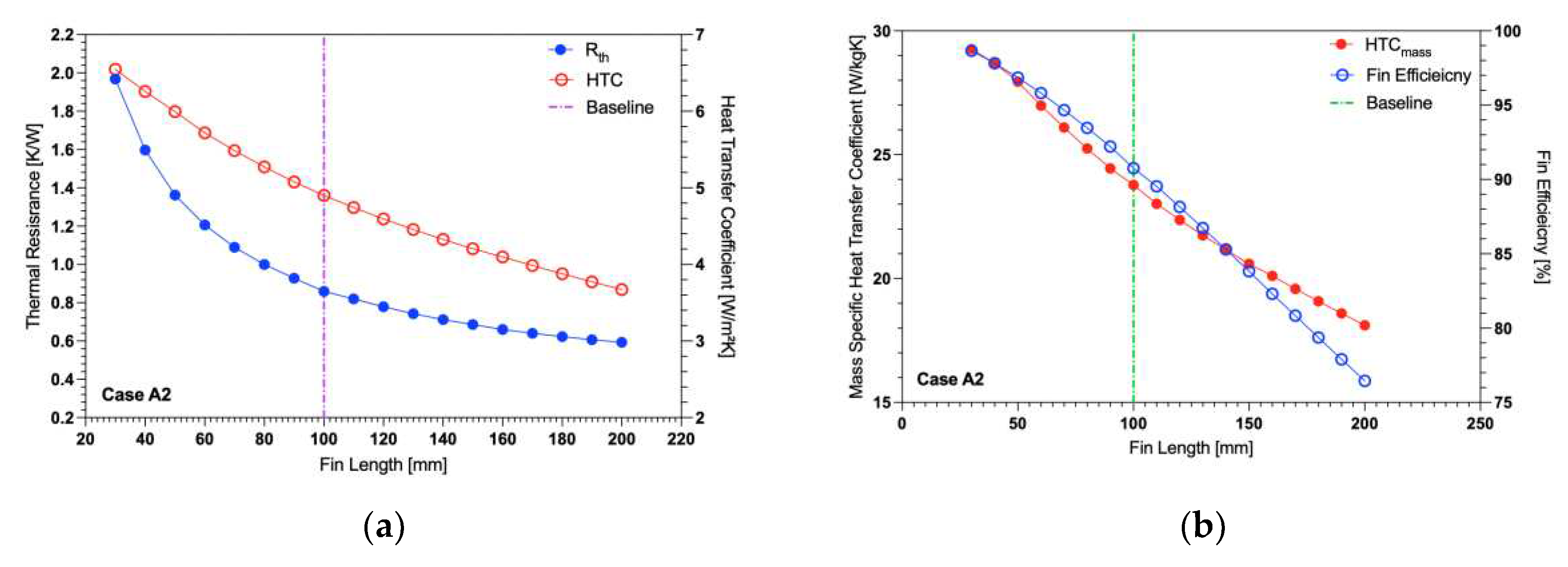
Figure 8 shows the variation of rectangular fin length with optimal spacing. The fin length was varied with the fin spacing set to the optimal value 9.09 mm that was found as a result of optimization. As the fin length increases, the fin array thermal resistance decreases, resulting in a higher rate of heat transfer. This is due to the increased surface area for longer fin, which allows provision for more heat to transfer (see Figure 8 (a) for details). As can be seen in Figure 8 (b), the fin efficiency drops significantly when the length of the fin increases. Since higher fin efficiency is more desirable as it improves thermal performance over a fixed area. The highest heat transfer coefficient is present when the fin length is shorter, this is also the case for the mass specific heat transfer coefficient.
Figure 8.
Variation of rectangular fin length with optimal spacing. (a) Heat transfer coefficient (HTC) and thermal resistance (Rth). (b) Percentage fin efficiency and mass specific heat transfer coefficient.
Figure 8.
Variation of rectangular fin length with optimal spacing. (a) Heat transfer coefficient (HTC) and thermal resistance (Rth). (b) Percentage fin efficiency and mass specific heat transfer coefficient.
3.2. Trapezoidal Fin
3.2.1. Design Case B1
Figure 9 shows the variation of trapezoidal fin lower length with optimal spacing for a midpoint length of 100 mm. As observed in Figure 9(a), the variation of the lower length of the trapezoidal fin heat sink showed that, when its value was set to 98 mm (corresponding to an upper length of 102 mm), the results showed a decrement in the thermal resistance (Rth) and increment in the heat transfer coefficient (HTC).
While the change in Rth and HTC was minor at a lower fin length of 98 mm compared to 100 mm, the different in performance compared to the baseline was significant (-4.7% for Rth and 0.2% for HTC). The volumetric flow rate was calculated by using the area-weighted average velocity passing through a plane in the middle of the fin and plotted as shown in Figure 9(b). Since the midpoint of the fin was fixed, the area of the plane remained constant throughout the bottom length variation. The volumetric flow rate peaks at a fin lower length of 90 mm. These thermal improvements at the local optimum may be due to this increase in flow rate for the configuration combined with the higher fin efficiency as can be seen in Figure 9(b).
3.2.2. Design Case B2
Figure 10 shows the variation of trapezoidal fin lower length with optimal spacing for a midpoint length of 50 mm. The testing is similar to case B1, but for a midpoint length of 50 mm. The behavior of the heat transfer coefficient and thermal resistance observed here with shorter fin was nearly identical to the one seen above. This confirms that the behavior is dependent rather on the fin lengths but on the angle of the shroud placed at the end of the fin that alters the performance of the fin array. A local optimal was found with a bottom fin length of 48 mm (corresponding to an upper length of 52 mm). At this length there was a decrease in the thermal resistance and an increase in the heat transfer coefficient as seen in Figure 10(a). Both Case B1 and B2 displayed optimal heat transfer when the trapezoidal fin was angled at 87.7° (i.e., 2.3° degrees from vertical), while only two fin midpoint lengths were tested. This seems to indicate that this may be the best angle for a shroud for a varying fin midpoint length. At this configuration the volumetric flow rate is close to its maximum for the length variation. Similarly, the fin efficiency also increases as the lower length of the fin decreases. The improved performance to the rectangular shape is likely due to a combination of these factors, i.e., increased fluid flow past the heated surface and a more efficient fin.
3.3. Curved Fin
3.3.1. Design Case C1
Figure 11 shows the variation of curved fin midpoint length with optimal spacing for the fin upper and lower lengths of 100 mm. As can be seen in Figure 11(a), as the fin’s midpoint length increases, the heat sink experiences a reduced thermal resistance thus increasing the overall heat transfer of the system. While this improvement is genuine, it is worth noting that as the fin midpoint length increases so does the fin’s surface area, which is directly proportional to the heat transferred. Interestingly, the improvement in thermal resistance begins to converge after a midpoint length of 120 mm even with an increasing area. This indicates the existence of a local optimum geometry for a convex curved fin. This local optimum may be due to the high flow rate present under these geometry conditions. The volumetric flow rate passing through the inside of the fin channel can be seen in Figure 11(b). The peak flow rate occurs at approximately 110 mm midpoint length, with only a minor decrease at 120 mm. Looking at the heat transfer coefficient as shown in Figure 11(a), it begins converging on a maximum as the fin midpoint length approaches 50 mm. The heat transfer coefficient is essentially a measure of how efficiently something dissipates heat, i.e., the higher the heat transfer coefficient the greater heat can be transferred for a fixed area. In the context of heat sinks, the size of them can often be factor of importance. Thus, designs that can transfer the same amount of heat but across a smaller area, and thus take up a smaller volume, are more desirable. Since that configuration of the curved fin showed potential promise as a more efficient design, the further geometry variations were focused on designs with a midpoint length of 50 mm.
3.3.2. Design Case C2
The midpoint height (i.e., the vertical distance from the bottom of the heat sink to the curved spline’s midpoint; see Figure 4) was varied from 20 mm to 80 mm. Any closer midpoint to the top or bottom of the profiles resulted in too extreme of a curve to be reliably meshed. The different permutations resulted in a change in the type of curve on the fin’s shroud. A midpoint height of 30 mm will produce a curved fin of equal area to a height at 70 mm due to the symmetry of the design and linearity of the height variation. The thermal resistance and heat transfer coefficient would be expected to be symmetrical as the midpoint height increases.
Interestingly, Figure 12 shows only a minor increase in the thermal resistance as the midpoint height increases. The opposite is true for the heat transfer coefficient, which decreases as the thermal resistance increases. While it may seem like a curve with a lower midpoint height provides the lowest thermal resistance and highest heat transfer coefficient, it should be noted that the numerical stability of the solution decreased significantly as the midpoint height varied in either direction from 50 mm, which may be indicative of unsteady flow separation or transition.
3.3.3. Design Case C3
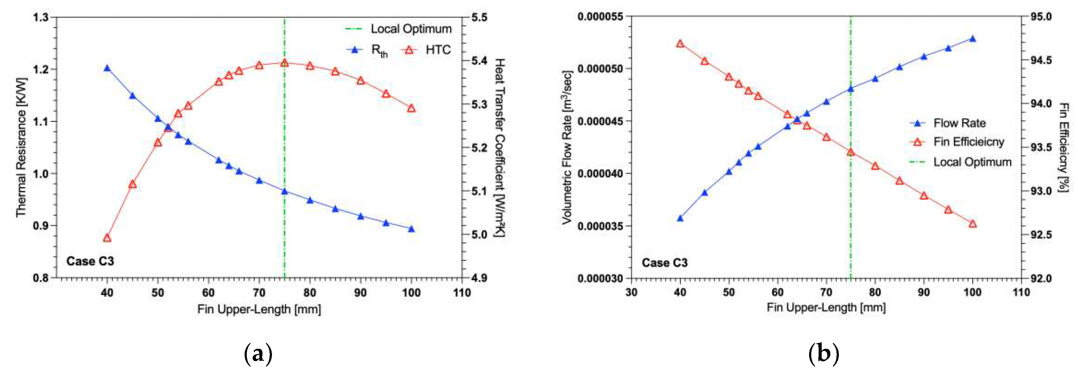
The fin’s bottom profile was fixed at a length of 100 mm while its midpoint length was fixed at 50 mm in the horizontal and vertical direction. Only the top profile length was allowed to vary. As the upper profile decreases from 100 mm the thermal resistance of the system increases. This is expected as the decrease in the upper length reduces the overall fin area. Interestingly, the heat transfer coefficient peaks at a value of 75 mm. This indicated the presence of a local optimum. Why this is the case is unclear as the maximum flow rate through the fin channel occurs at a length of 100 mm and a maximum fin efficiency at 40 mm. The answer may be found in the resemblance of this geometry to the hyperbolic curve found in natural draft cooling towers. The shape of these cooling towers forces the rising hot air through a narrow throat section resulting in an acceleration of the fluid. To assess whether flow unsteadiness or transition would be observed in such configurations, this same case was run using the Transition-SST turbulence model and compared to the laminar flow model results. When run with the turbulent model, the fluid velocities inside the fin channels were significantly lower with the maximum velocity through the mid-plane of the fin being 0.158 m/s and 0.076 m/s for the laminar and turbulent model respectively. While the fluid flow was much slower inside the fin channel for the turbulent model, outside the speed of the fluid was significantly increased. The transition model resulted in a higher base temperature of 359.1 K compared to 338.4 K for the laminar model.
Figure 13.
Variation of curved fin upper length with optimal spacing for midpoint length fixed at 50 mm and lower length of 100 mm. (a) Heat transfer coefficient (HTC) and thermal resistance (Rth). (b) Percentage fin efficiency and volumetric flow rate.
Figure 13.
Variation of curved fin upper length with optimal spacing for midpoint length fixed at 50 mm and lower length of 100 mm. (a) Heat transfer coefficient (HTC) and thermal resistance (Rth). (b) Percentage fin efficiency and volumetric flow rate.
3.3.4. Design Case C4
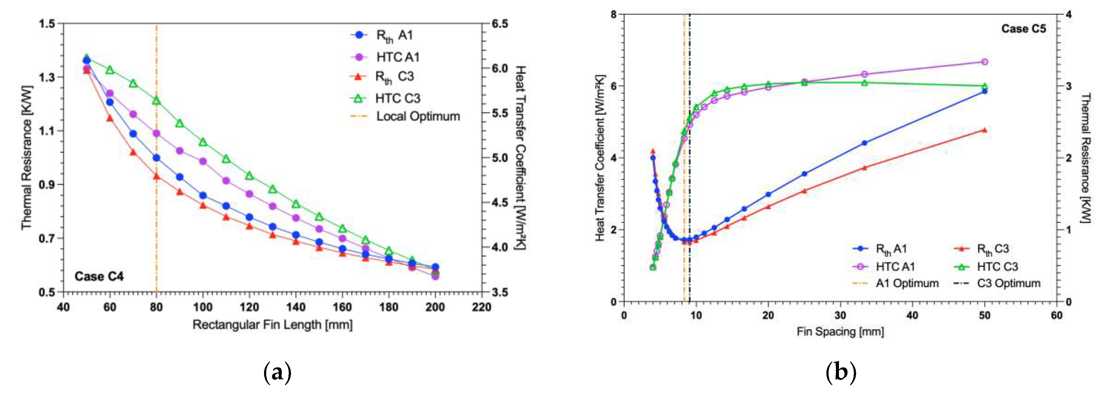
In Figure 14(a), the heat transfer coefficient and thermal resistance of rectangular and curved fins for varying lengths are plotted. The x-axis indicates the length of the rectangular fins, with the curved fin at that point plotted that represents equal area to the corresponding length of rectangular fin. By comparing these two fin designs based on an equal area, the thermal improvements of one design over the other are easier to see. As is expected, the thermal resistance of both arrays is at its lowest when the fin length is at 200 mm. This is obviously the configuration with the highest fin surface area so would be expected to provide the largest temperature drop for the heat source. The heat transfer coefficient is at its maximum when the fin length is 50 mm. This is where the fins have their highest fin efficiency and can dissipate the most heat per unit area. For nearly all rectangular fin lengths tested, the curved fin with equivalent area provides a decreased thermal resistance and increased heat transfer coefficient demonstrating its design superiority over the baseline design. The difference in performance is not constant with the maximum improvements in the design when the rectangular fin has a length of 80 mm. The curved fin for this length has a decreased thermal resistance of 6.6% and an increased heat transfer coefficient of 5.6%.
Figure 14.
Variation of curved fin midpoint length with optimal spacing with upper and lower length of 100 mm. (a) The heat transfer coefficient and thermal resistance are plotted for variation of the mid fin length. (b) The fin efficiency and volumetric flow rate through the fin channel for variation of the mid fin length.
3.3.5. Design Case C5
The behavior of heat transfer coefficient and thermal resistance for curved fin array with varying fin spacing is similar to that of the rectangular fins for the same spacing variation. For the curved fin there exists a fin spacing that minimizes the array’s thermal resistances. As the spacings decreases from that optimal spacing, the thermal resistance increases dramatically while the heat transfer coefficient decreases in the same manner. This is nearly identical to the behavior expected of a rectangular fin and can be seen in the closeness in values in Figure 14(b). As the spacing increases beyond the optimum, the heat transfer coefficient plateaus after a spacing of approximately 20 mm, while the thermal resistance steadily increases. This behavior is similar to that displayed by the rectangular fin case except for the rectangular fins providing a more pronounced change in thermal resistance and heat transfer coefficient for an increasing fin spacing than the curved fin case. Due to the array being a fixed width, the spacings available are limited to those values which correspond to a whole number of fins on the base plate. Because of this, the optimal spacing of two fins cannot just be considered, but also the whole number of fins resulting from that spacing. As a result, there may exist an optimal spacing between two fins, but it falls between the increments available for the specific base plate size chosen for this study (i.e., 100 mm x 100 mm). In Figure 14(b) the optimal fin spacing for both the rectangular and novel curved fin design has been dictated by the spacing that minimizes the thermal resistance for the array. While this is a reasonable definition, it does not fully consider the efficiency of the design. The difference between the thermal resistance at 8.33 mm and 9.09 mm is essentially negligible while the increase in the heat transfer coefficient is significant. A more informed decision would suggest that the optimal fin spacing for both the baseline and curved fin would be at 9.09 mm where the thermal resistance is sufficiently low, but the heat transfer coefficient is also at a high level.
3.4. Angled Fin (Design Cases D1, D2)
The optimized rectangular baseline fin case was compared against the optimized angled fin case adopted from Zhang et al. [3], for identical heat inputs and boundary conditions. Their geometrical parameters were chosen to be identical apart from their respective fin arrangements and fin spacings. The fins were tested against one another for three different simulation setups as follows: (i, ii) Laminar flow model with discrete ordinance (DO) radiation (i) disabled and (ii) enabled, and the (iii) transition-SST model with radiation disabled. This leads to a total of six simulations, the results of which are summarized in Table 6, Table 7 and Table 8. The percentage difference for the thermal resistance and heat transfer coefficient between each tested case with the baseline rectangular fin (for laminar with no radiation) are also shown in Table 6. A better design is one that produces a decrease in the thermal resistance compared to the baseline (i.e., a negative percentage difference). An increase in the heat transfer coefficient is also desirable (i.e., a positive percentage difference).
For the laminar flow model without radiation, the rectangular fin array (A1) provided a significantly lower thermal resistance than the angled fins (except for the case D2 with 55 mm fin length). Similarly, case A1 provided a significantly higher heat transfer coefficient. The relative comparison between the angled fins to the baseline in terms of heat transfer coefficient may not be appropriate here because as noticed in Table 6, for case D2 with 55 mm fin length, even though the thermal resistance and the heat sink’s base temperature are lower, the calculated heat transfer coefficient is lower than that of the baseline rectangular fins. The same is the case for other tested simulations as well. Moreover, the angled fins with pressure outlet boundary condition (case D2) on one side and symmetry on the other side enhances the heat transfer performance in comparison with 100 mm fin length case D1 for all the tested simulations as seen in Table 6, Table 7 and Table 8.
The temperature of the heat sink’s base for case D2 is lowered by 3.9 K than that of the baseline rectangular fins. This could be attributed to a reduction in average fluid temperature within the heat sink volume, as warm air is allowed to escape out the side through the angled fin spacing, resulting in the induction of generally cooler air in the normal direction to the heat sink’s base. In other angled fin cases, this effect is likely suppressed due to the increased number of angled fins compared to the rectangular array. However, the higher number of fins positioned at an angle to the vertical direction may also provide a higher impedance to the fluid flow reducing the overall fluid velocities achievable inside the fin channels. This is evidenced by the average velocity recorded above each fin array, 0.0650 m/s for the angled fins (100 mm fin length case D1) compared to 0.0974 m/s for the optimized rectangular fin array.
Upon enabling the DO radiation model, a large drop in the heat sink base temperature was recorded for both fin designs as shown in Table 7 in comparison with the cases mentioned in Table 6. This corresponded to a significant decrease in thermal resistance by 10.9% and increase in the heat transfer coefficient by 12.2% for the baseline case A1. Similarly, the angled fin cases also exhibited same behavior. By enabling the DO model, heat transfer by radiation is included into the overall transfer of heat from the heat sink to the surroundings. This additional mode of heat transfer increases the overall amount of energy that the heat sink can dissipate thus decreasing the base temperature. Like in the first simulation case, the angled fins as in case D2 here as well performed significantly better with a base temperature of 340.5 K compared to 345.7 K for the rectangular fins.
When tested with the Transition-SST turbulence model, the highest individual improvements are achieved for each of the tested cases in comparison to its corresponding Rth, HTC and temperatures mentioned in Table 6 and Table 7. However, as shown in Table 8, the difference in this improvement when compared to the baseline case was observed to be smallest. In comparison with the laminar flow results of Table 6, the angled fins here in case D1 with 55 mm fin length showed a temperature drop of almost 19 K compared to a 10 K drop observed for the rectangular fin case A1. This results in an increased heat transfer coefficient that is mainly due to a turbulence model being used over the laminar model. Even in globally laminar flow (with a Rayleigh number below ), the transition-SST model could predict locally transitional or turbulent flow in certain regions. The model could thus predict more chaotic motion and efficient fluid mixing, resulting in higher heat transfer rates between the heat sink and the fluid [18].
The findings of Zhang et al. [3] are not entirely confirmed by these results. The closest comparison would be case D2 (angled fins with symmetry on one side and pressure outlet on the other side) compared to case A1. Based on the present results, case D2 only outperforms the rectangular fins for a shorter fin length of 55 mm. However, for longer fin lengths (100 mm), this proposition fails as the D2 heat sink’s base temperature almost matches that of the rectangular array (A1). Moreover, case D1 with symmetry on both sides performed worse altogether, which seems to indicate that the angled fin approach would not be beneficial for a general heat sink base area, but rather that specific combinations of base dimensions (and possibly Rayleigh number) could lead to enhancements as observed in Zhang et al. [3].
4. Discussion
4.1. Chilton-Colburn Analogy
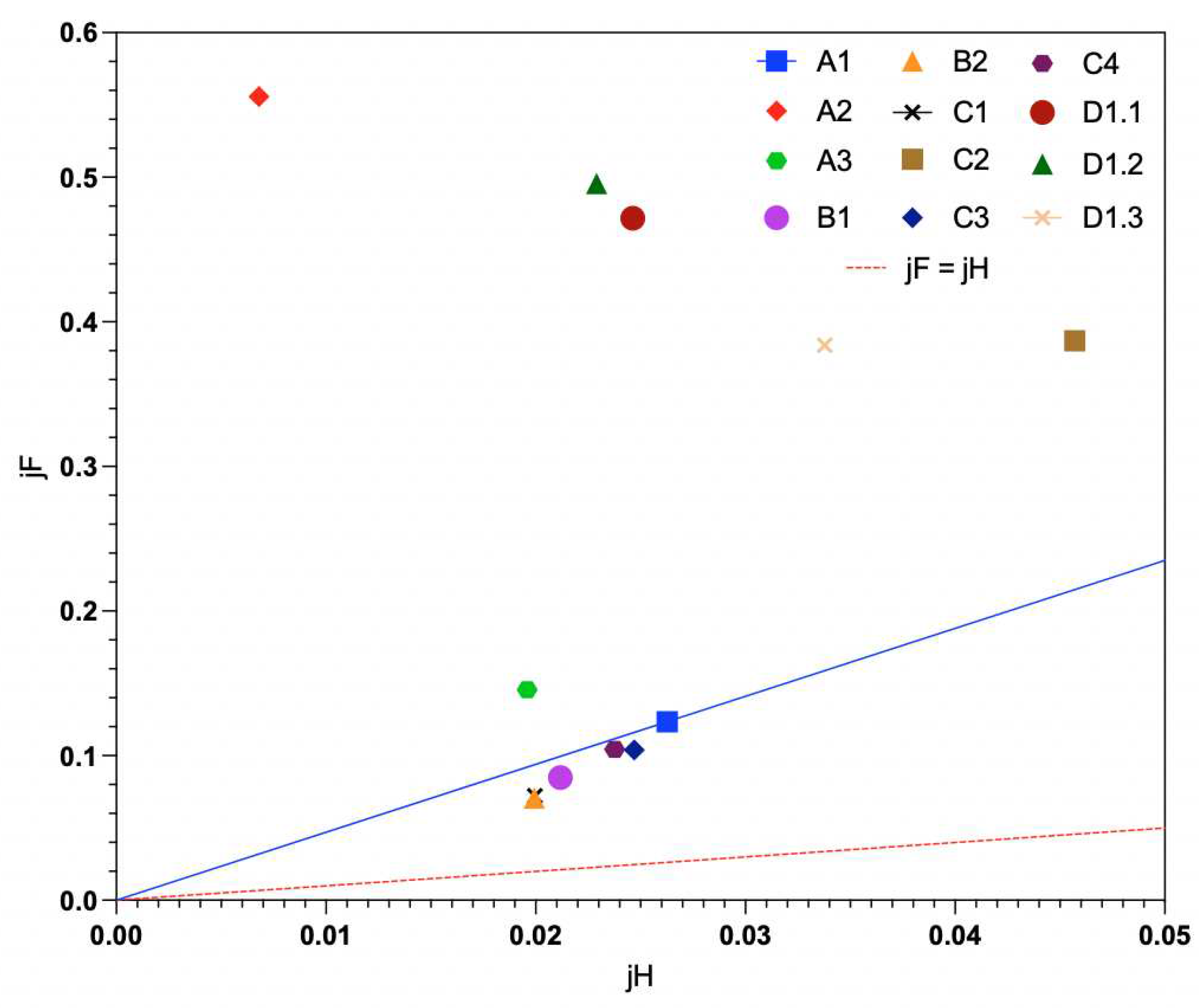
The performance of heat sink designs can also be assessed using the Chilton-Colburn analogy. Using Equation (6), and can be calculated. Although this analogy between heat and momentum transfer is only expected to hold exactly for certain canonical configurations (e.g., laminar flow over a flat plate), one could classify “good” heat sink designs as cases where the ratio / increases with respect to some baseline, meaning that the rate of heat transfer is higher for the same amount of fluid friction, with the converse being true for a reduction in /. The spread in results from the different cases investigated here interestingly shows the better performing cases located closer to the red dashed line in Figure 13 where or . In Figure 13, data markers that are located lower down or more to the right on the graph represent better designs. The angled fins with all the simulated cases: laminar flow with no radiation, laminar flow with radiation and transition-SST with no radiation were also included in Figure 13 with notations .1, .2 and .3 respectively.
Figure 13.
Plot of against for all the design cases (cases A2 and A3 refer to rectangular fin of length 100 mm set to a spacing of 4 mm and 20 mm respectively i.e., below and above the optimal spacing).
Figure 13.
Plot of against for all the design cases (cases A2 and A3 refer to rectangular fin of length 100 mm set to a spacing of 4 mm and 20 mm respectively i.e., below and above the optimal spacing).
4.2. Optimal Design and the Choice of Objective Function
The best-case scenario for each of the design cases was taken and compared against the optimally spaced rectangular fin baseline in terms of thermal resistance and heat transfer coefficient. The percentage difference in the thermal performance of heat sink’s array for each of the subsequent design cases in comparison to the rectangular fin baseline were also calculated. Table 9 details the varying thermal performance of the different design cases when configured to their respective local optima. Several trends can be observed from the variation of thermal performance based on the differing geometries:
- Firstly, the thermal resistance is inherently linked to the total heat transfer area. Case B1 compared to B2 has a significantly lower thermal resistance and thus lower temperature. Similarly, Case C1 which provides the lowest thermal resistance out of the 12 cases listed in Table 9 also has the highest surface area. The converse of this is true for the heat transfer coefficient with more compact designs producing higher heat transfer coefficients given their higher fin efficiencies due to their closer proximity to the heat source.
- The most marked improvement is arguably seen in case C4. This design has the same exact area as the baseline yet provides a noteworthy decrease in the thermal resistance while simultaneously improving the heat transfer coefficient. This proves that the design itself is more efficient and is not merely reflecting a performance enhancement through an increase in heat transfer area.
- The ‘optimal’ design is highly dependent on the relevant objective function and constrictions placed on a specific scenario. For example, in light-weight applications where the mass of the heat sink is to be limited, then a design with a high heat transfer coefficient per unit mass takes priority. Whereas if the overall thermal performance of the system is the priority and there are no limitations on size then a larger area fin such as Case C1 would prove to be the optimal.
4.3. Non-Dimensional Analysis and Scaling of Design Cases
In Figure 15, the horizontal axis shows the averaged fin length of the trapezoidal (Case B1 and B2) and curved (Case C1 to C5) fins, normalized by the fixed fin height of the baseline Case A1 ( mm). For clarity, ‘height’ refers to the direction parallel to gravity and ‘length’ refers to the direction perpendicular to the base area, i.e., perpendicular to gravity. Similarly, the vertical axes in Figure 15 show the thermal resistance, heat transfer coefficient, heat transfer coefficient by mass, and fin efficiency, all normalized by the values of the baseline case (Case A1). Recall that design cases B1 and C4 are the only two cases that have shown simultaneous improvement of all the performance parameters, with C4 outperforming B1. The results of design case C4 have shown better performance than the baseline rectangular fin design for thermal resistance, heat transfer coefficient, heat transfer coefficient by mass, and fin efficiency for all the simulated / ratios. The optimal performance is achieved at an / ratio of 0.8 (approximately), with local maxima and minima for the performance parameters. However, a significant decline in the performance is observed when there is a decrease or increase in the / ratio. Hence, a design recommendation of /= 0.8 has emerged for design case C4.
The obtained scaling factors could be used for designing these two novel heat sinks for any given dimensions without running further simulations, as long as the Rayleigh number, ambient conditions and fluid properties remain comparable. It is important to note that this is a general strategy and can be adopted for the design of any new natural convection heat sink designs. For instance, at a given heat load condition, the effective heat transfer coefficient will be obtained by multiplying it with the scaling factor in Equation (4) and back calculating the optimized spacing using Equations (3). However, the validity of this hypothesis must be further tested and is the subject of future work.
5. Conclusions
Based on a literature review on natural convection heat sink design, there is currently no established strategy for creating a new heat sink that outperforms a classical rectangular plate fin array design with optimized fin spacing. The optimal fin spacing for a baseline rectangular fin case studied here is between 8.33 mm and 9.09 mm. This value is obtained by minimizing the thermal resistance for a given base area (100 mm x 100 mm) and thermal boundary conditions (air at atmospheric pressure and 300 K, uniform heat flux of 4000 W/m2 at the base) and simultaneously maintaining a high average heat transfer coefficient. These values are in close agreement with the semi-empirical model of Elenbaas [2]. This optimized baseline rectangular fin generally performs better than the proposed novel designs in the literature. In specific conditions, some enhancement is observed [3] which was partly confirmed in this study. However, it is difficult to achieve a consistent marked improvement over the optimized rectangular fin baseline case. That said, there is still scope for designing novel heat sinks which can outperform the optimized baseline rectangular fins. Trapezoidal and curved fin shapes are two such proposed fin designs that outperform baseline rectangular fins, yet still represent very basic and easily manufactured geometries. Case C1 with curved fins had the most pronounced reduction in thermal resistance at -5.5%, albeit with a 4.5% lower heat transfer coefficient. It is worth noting that this design had a larger surface area than the rectangular baseline. On the other hand, for a fixed surface area, the hyperbolic-like curved fins of Case C4 featured the most significant reduction in thermal resistance compared to the baseline at -4.1% and an increase in average heat transfer coefficient by +4.4%. The study also examined if the performance enhancements remained constant at varying fin length. The maximum improvement was achieved at a rectangular fin length of 80 mm. The curved fin Case C4 with 80 mm fin length produced a -6.6% reduction in thermal resistance and a +5.6% increase in heat transfer coefficient.
Author Contributions
Conceptualization, O.M., S.M.A., R.N. and T.P.; methodology, O.M., S.M.A., R.N. and T.P.; software, O.M. and R.N.; validation, O.M.; formal analysis, O.M., R.N., S.M.A.; resources, T.P.; data curation, O.M. and R.N.; writing—original draft preparation, O.M.; writing—review and editing S.M.A., R.N. and T.P.; visualization, O.M. and R.N.; supervision, S.M.A. and T.P. All authors have read and agreed to the published version of the manuscript.
Funding
This research was partly funded by Trinity College Dublin. This publication has emanated from research supported in part by a research grant from Science Foundation Ireland (SFI) and is co-funded under the European Regional Development Fund under Grant Number 13/RC/2077_P2.
Data Availability Statement
The data presented in this study are available on request from the corresponding author.
Conflicts of Interest
The authors declare no conflict of interest.
References
- Balaji, C.; Srinivasan, B.; Gedupudi, S. Chapter 6 - Natural convection. In Heat Transfer Engineering. Academic Press: London, U.K., 2021; pp. 173–198. [Google Scholar]
- Elenbaas, W. Heat dissipation of parallel plates by free convection. Physica 1942, 9, 1–28. [Google Scholar] [CrossRef]
- Zhang, K.; Li, M.-J.; Wang, F.-L.; He, Y.-L. Experimental and numerical investigation of natural convection heat transfer of W-type fin arrays. Int J Heat Mass Transfer 2020, 152, 119315. [Google Scholar] [CrossRef]
- Jaffer, A. Natural convection heat transfer from an isothermal plate. Thermo 2023, 3, 148–175. [Google Scholar] [CrossRef]
- Florio, L.; Harnoy, A. Combination technique for improving natural convection cooling in electronics. Int J Therm Sci 2007, 46, 76–92. [Google Scholar] [CrossRef]
- Bar-Cohen, A.; Rohsenow, W. M. Thermally optimum spacing of vertical, natural convection cooled, parallel plates. J Heat Transfer 1984, 106, 116–123. [Google Scholar] [CrossRef]
- Yüncü, H.; Anbar, G. An experimental investigation on performance of rectangular fins on a horizontal base in free convection heat transfer. Heat Mass Transfer 1998, 33, 507–514. [Google Scholar] [CrossRef]
- Bar-Cohen, A.; Iyengar, M.; Kraus, A. D. Design of optimum plate-fin natural convective heat sinks. J Electron Packag, 2003, 125, 208–216. [Google Scholar] [CrossRef]
- Chen, L.; Yang, A.; Feng, H.; Ge, Y.; Xia, S. Constructal design progress for eight types of heat sinks. Sci China Technol Sci, 2020, 63, 879–911. [Google Scholar] [CrossRef]
- Ray, R.; Mohanty, A.; Patro, P.; Tripathy, K. C. Performance enhancement of heat sink with branched and interrupted fins. Int Comm Heat Mass Transfer, 2022, 133, 105945. [Google Scholar] [CrossRef]
- Chang, S.-W.; Wu, H.-W.; Guo, D.-Y.; Shi, J. J.; Chen, T.-H. Heat transfer enhancement of vertical dimpled fin array in natural convection. Int J Heat Mass Transfer, 2017, 106, 781–792. [Google Scholar] [CrossRef]
- Joo, Y.; Kim, S. J. Comparison of thermal performance between plate-fin and pin-fin heat sinks in natural convection. Int J Heat Mass Transfer, 2015, 83, 345–356. [Google Scholar] [CrossRef]
- Saghir, M. Z.; Ghalayini, I. Thermohydraulic performance of chevron pin-fins. Fluids, 2022, 7, 195. [Google Scholar] [CrossRef]
- Al-Neama, A. F.; Khatir, Z.; Kapur, N.; Summers, J.; Thompson, H. M. An experimental and numerical investigation of chevron fin structures in serpentine minichannel heat sinks. Int J Heat Mass Transfer, 2018, 120, 1213–1228. [Google Scholar] [CrossRef]
- Zhu, X.; Haglind, F. Relationship between inclination angle and friction factor of chevron-type plate heat exchangers. Int J Heat Mass Transfer, 2020, 162, 120370. [Google Scholar] [CrossRef]
- Welling, J. R.; Wooldridge, C. B. Free convection heat transfer coefficients from rectangular vertical fins. J Heat Transfer, 1965, 87, 439–444. [Google Scholar] [CrossRef]
- El Ghandouri, I.; El Maakoul, A.; Saadeddine, S.; Meziane, M. Design and numerical investigations of natural convection heat transfer of a new rippling fin shape. Appl Therm Eng, 2020, 178, 115670. [Google Scholar] [CrossRef]
- Bergman, T. L.; Lavine, A. S.; Incropera, F. P.; DeWitt, D. P. Fundamentals of Heat and Mass Transfer, 7th ed.; John Wiley & Sons: Hoboken, N.J., USA, 2011. [Google Scholar]
- ANSYS, ANSYS Fluent Theory Guide. Ansys Inc., 2009.
Figure 1.
Schematic representation of the full heat sink (left) and the computational geometry (right) adopted for CFD simulations. Not shown to scale. Gravity acts in the downward or negative -direction.
Figure 1.
Schematic representation of the full heat sink (left) and the computational geometry (right) adopted for CFD simulations. Not shown to scale. Gravity acts in the downward or negative -direction.
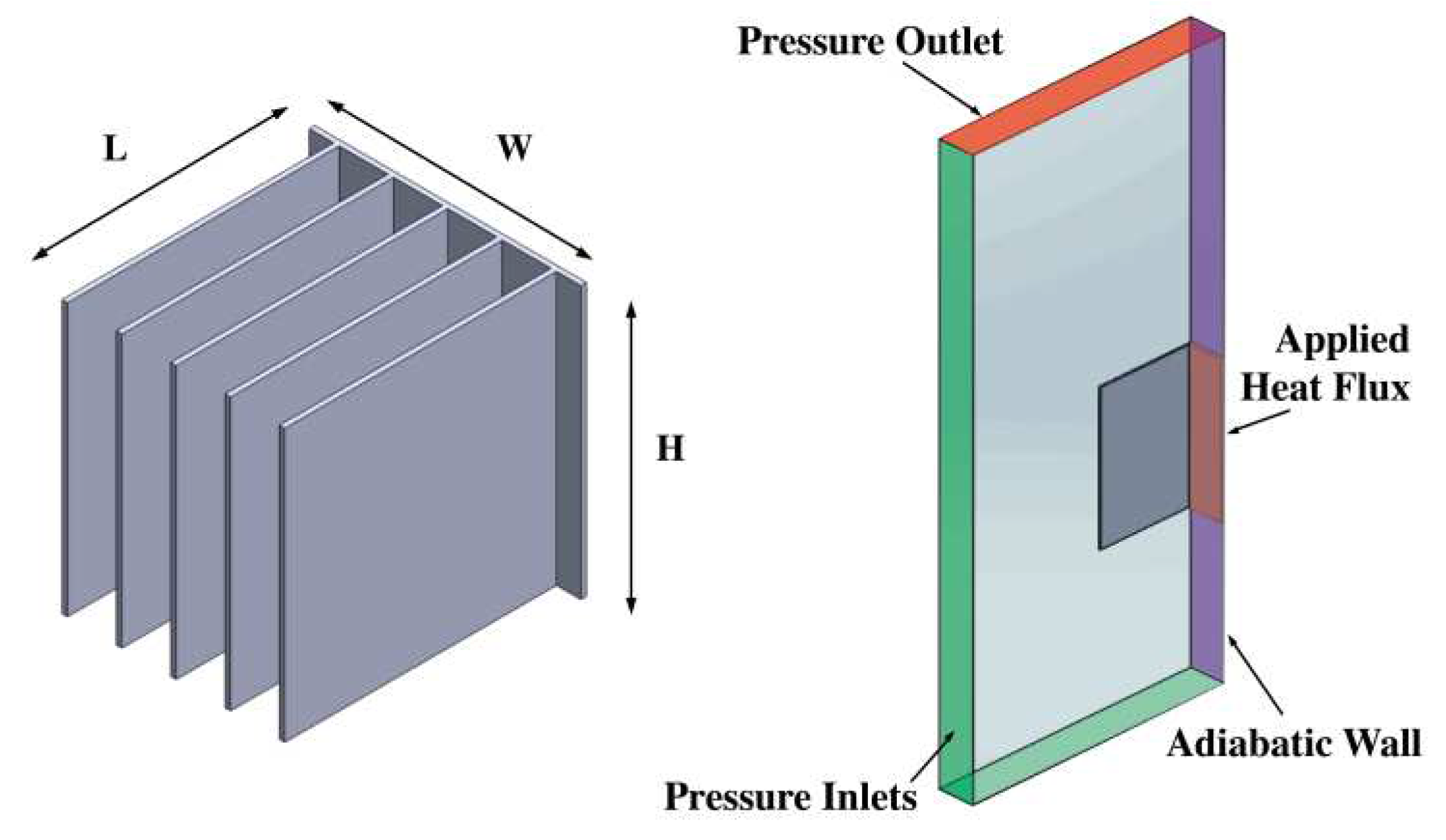
Figure 2.
Mesh convergence study to identify sufficiently small element size for case A1 (see Table 3, Figure 3).
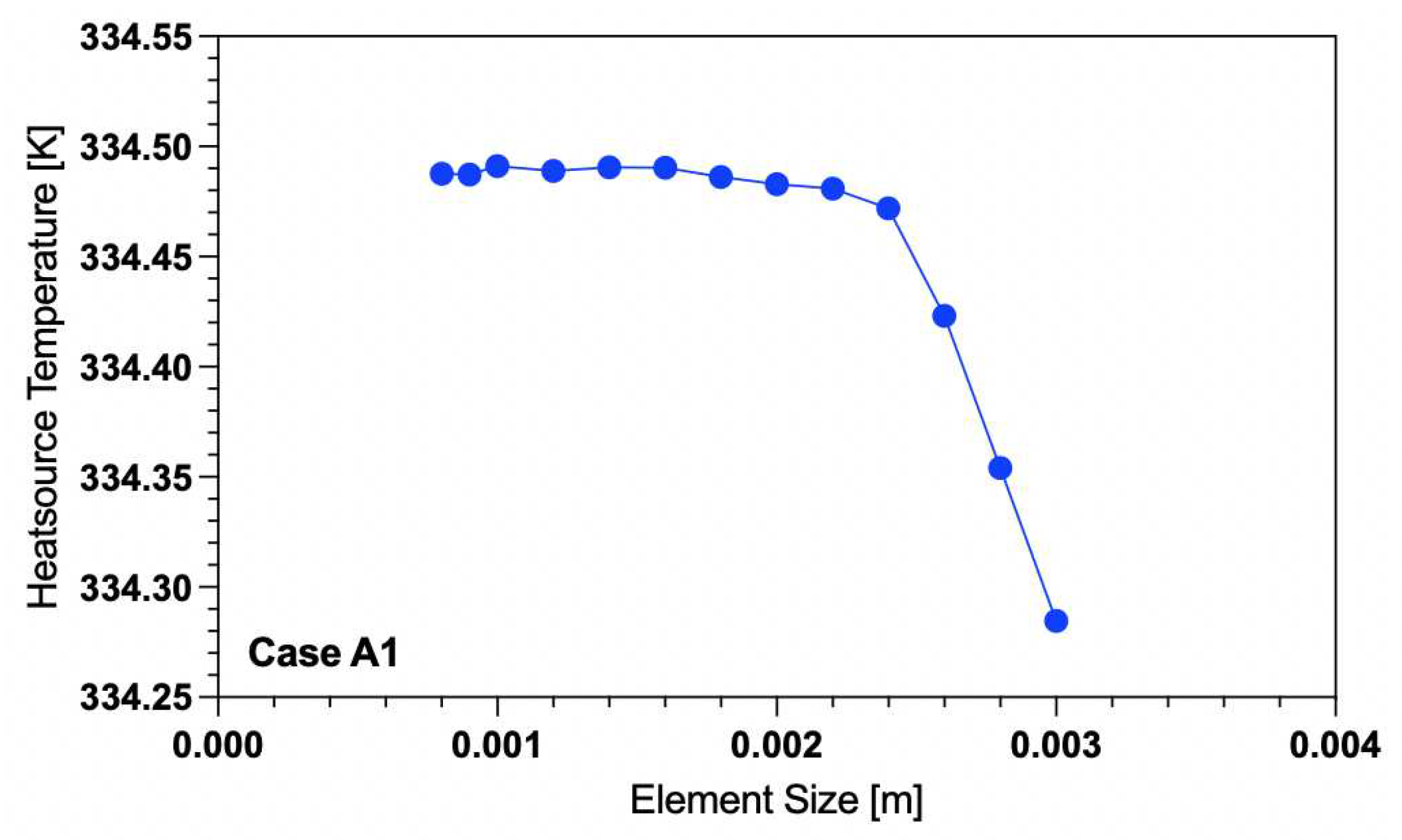
Figure 3.
Schematic representation of all the design cases used with their respective design codes.
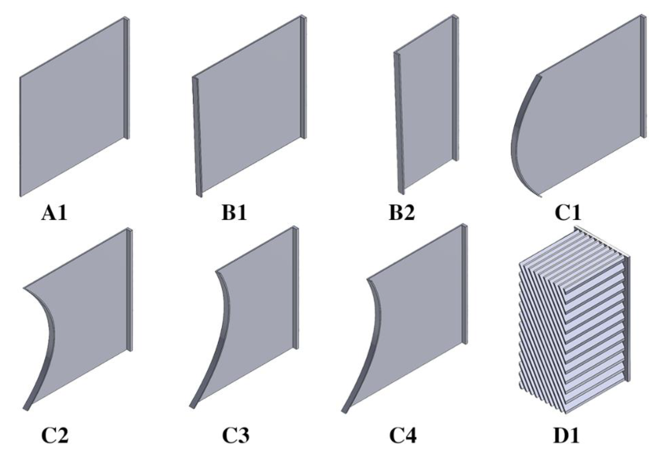
Figure 4.
Boundary sketches used to generate fin shapes for trapezoidal and curved fin design cases. (a) The trapezoidal fin boundary sketch representing a possible variation of fin midpoint length and fin lower length corresponding to B1 and B2. (b) The curved fin boundary sketch representing a possible variation of the upper and lower length of the fin, and the x-y position of the curve’s midpoint corresponding C1 to C4.
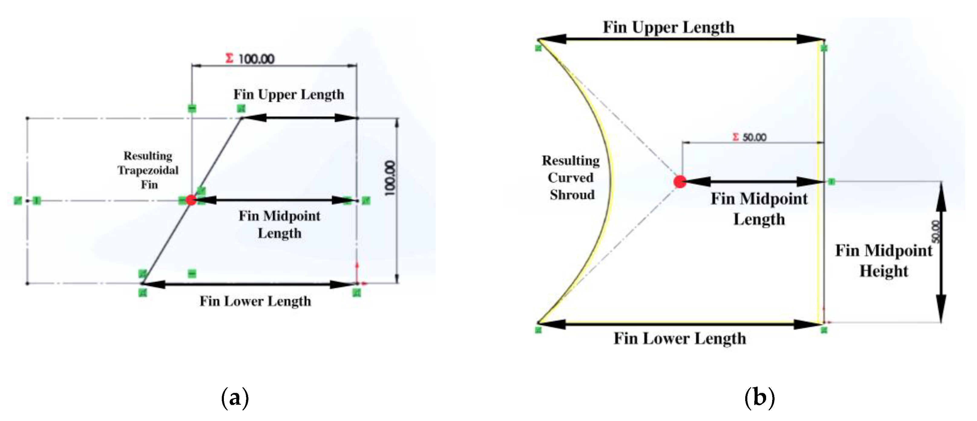
Figure 5.
Angled fin adjusted domain used for the study.
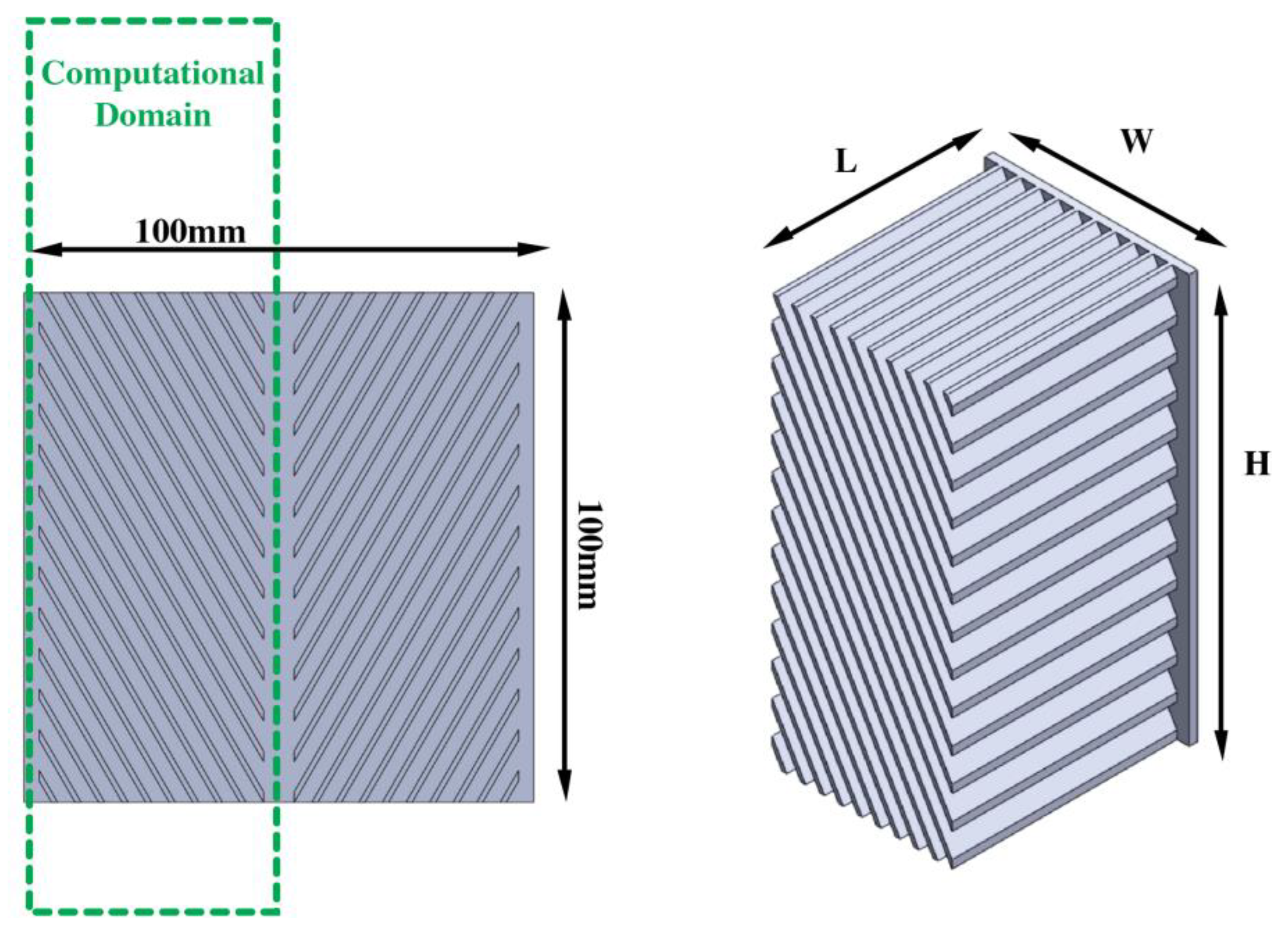
Figure 6.
Angled fin design cases with codes D1 (left) and D2 (right) having different computational domains. Not shown to scale.
Figure 6.
Angled fin design cases with codes D1 (left) and D2 (right) having different computational domains. Not shown to scale.
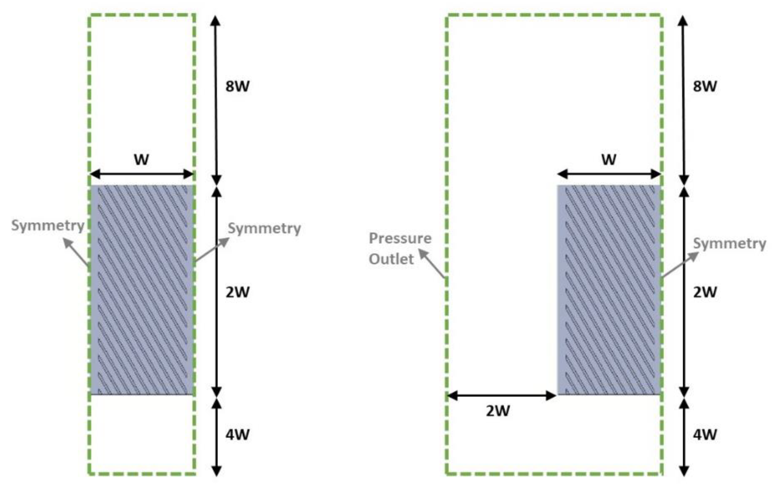
Figure 7.
Validation of variation of fin spacing for rectangular fin with the Elenbaas [2] semi-empirical correlation.
Figure 7.
Validation of variation of fin spacing for rectangular fin with the Elenbaas [2] semi-empirical correlation.
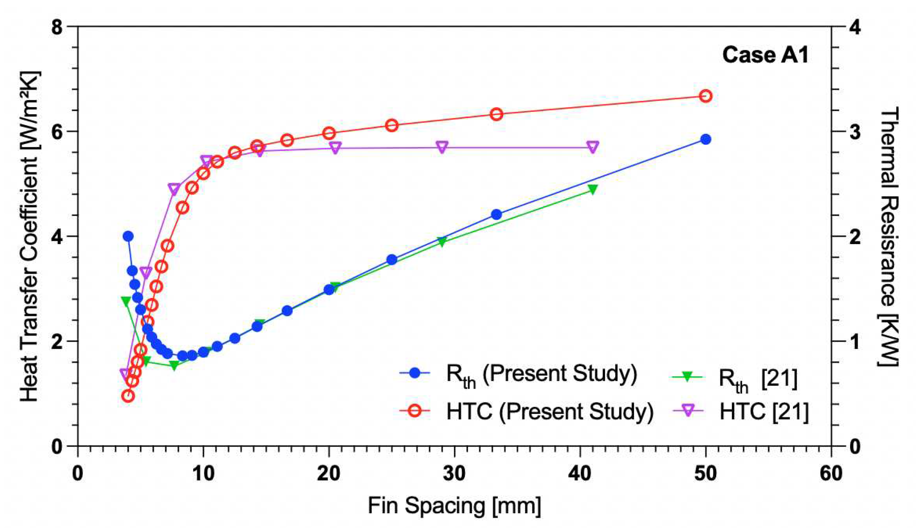
Figure 9.
Variation of trapezoidal fin lower length with optimal spacing for a midpoint length of 100 mm. (a) Heat transfer coefficient (HTC) and thermal resistance (Rth). (b) Percentage fin efficiency and volumetric flow rate.
Figure 9.
Variation of trapezoidal fin lower length with optimal spacing for a midpoint length of 100 mm. (a) Heat transfer coefficient (HTC) and thermal resistance (Rth). (b) Percentage fin efficiency and volumetric flow rate.
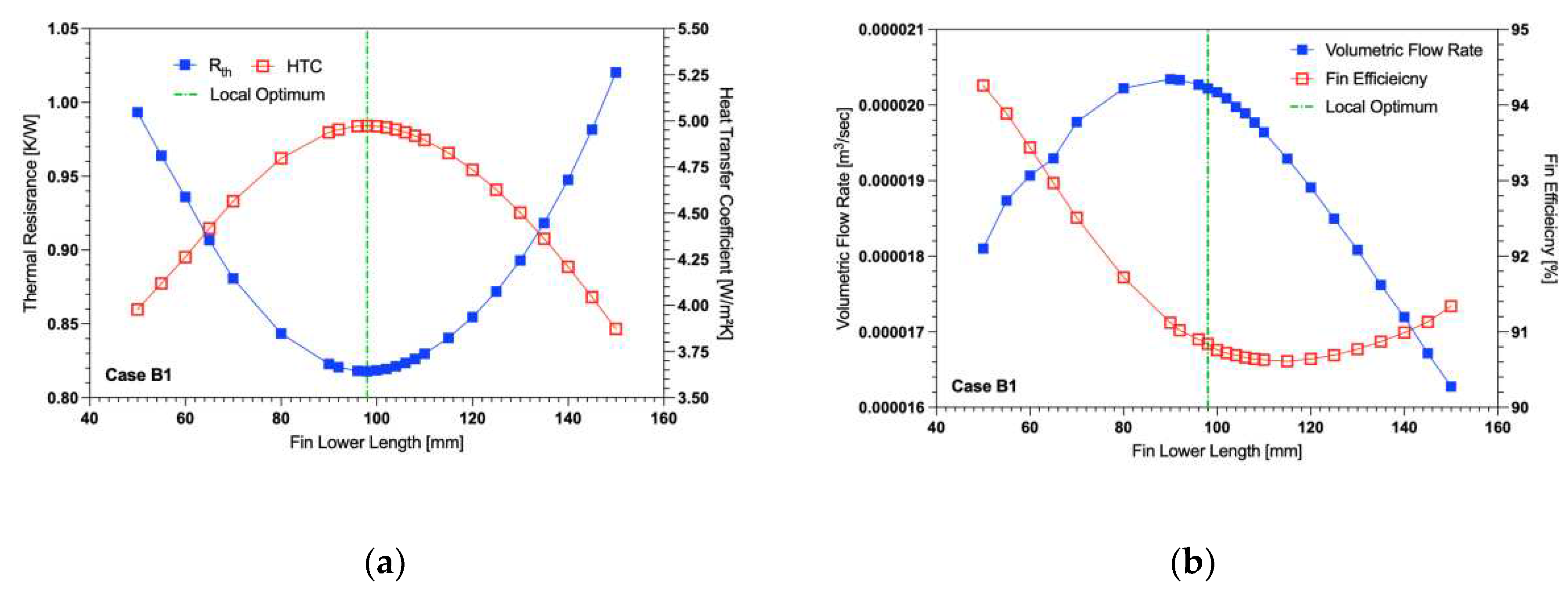
Figure 10.
Variation of trapezoidal fin lower length with optimal spacing for a midpoint length of 50 mm. (a) Heat transfer coefficient (HTC) and thermal resistance (Rth). (b) Percentage fin efficiency and volumetric flow rate.
Figure 10.
Variation of trapezoidal fin lower length with optimal spacing for a midpoint length of 50 mm. (a) Heat transfer coefficient (HTC) and thermal resistance (Rth). (b) Percentage fin efficiency and volumetric flow rate.
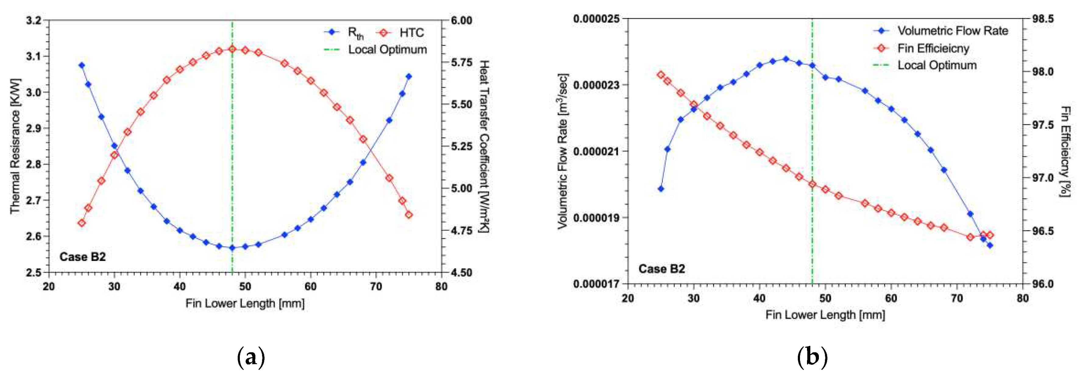
Figure 11.
Variation of curved fin midpoint length with optimal spacing for the fin upper and lower lengths of 100 mm. (a) Heat transfer coefficient (HTC) and thermal resistance (Rth). (b) Percentage fin efficiency and volumetric flow rate.
Figure 11.
Variation of curved fin midpoint length with optimal spacing for the fin upper and lower lengths of 100 mm. (a) Heat transfer coefficient (HTC) and thermal resistance (Rth). (b) Percentage fin efficiency and volumetric flow rate.
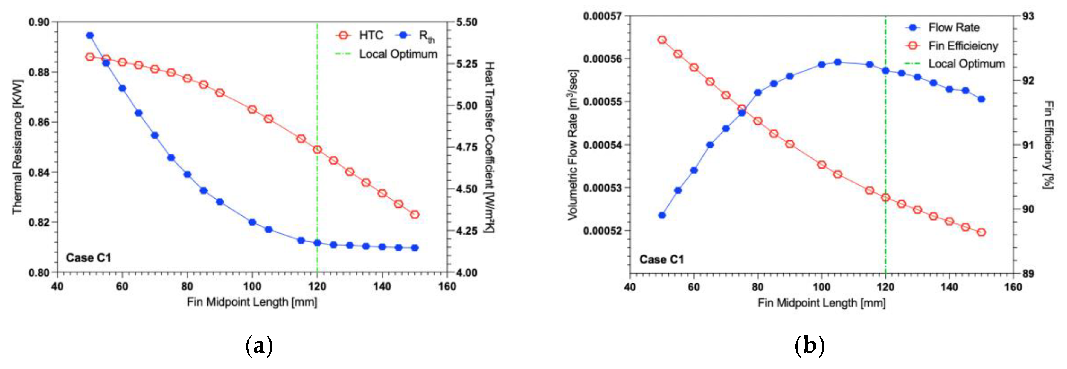
Figure 12.
Heat transfer coefficient (HTC) and thermal resistance (Rth) for variation of curved fin midpoint height.
Figure 12.
Heat transfer coefficient (HTC) and thermal resistance (Rth) for variation of curved fin midpoint height.
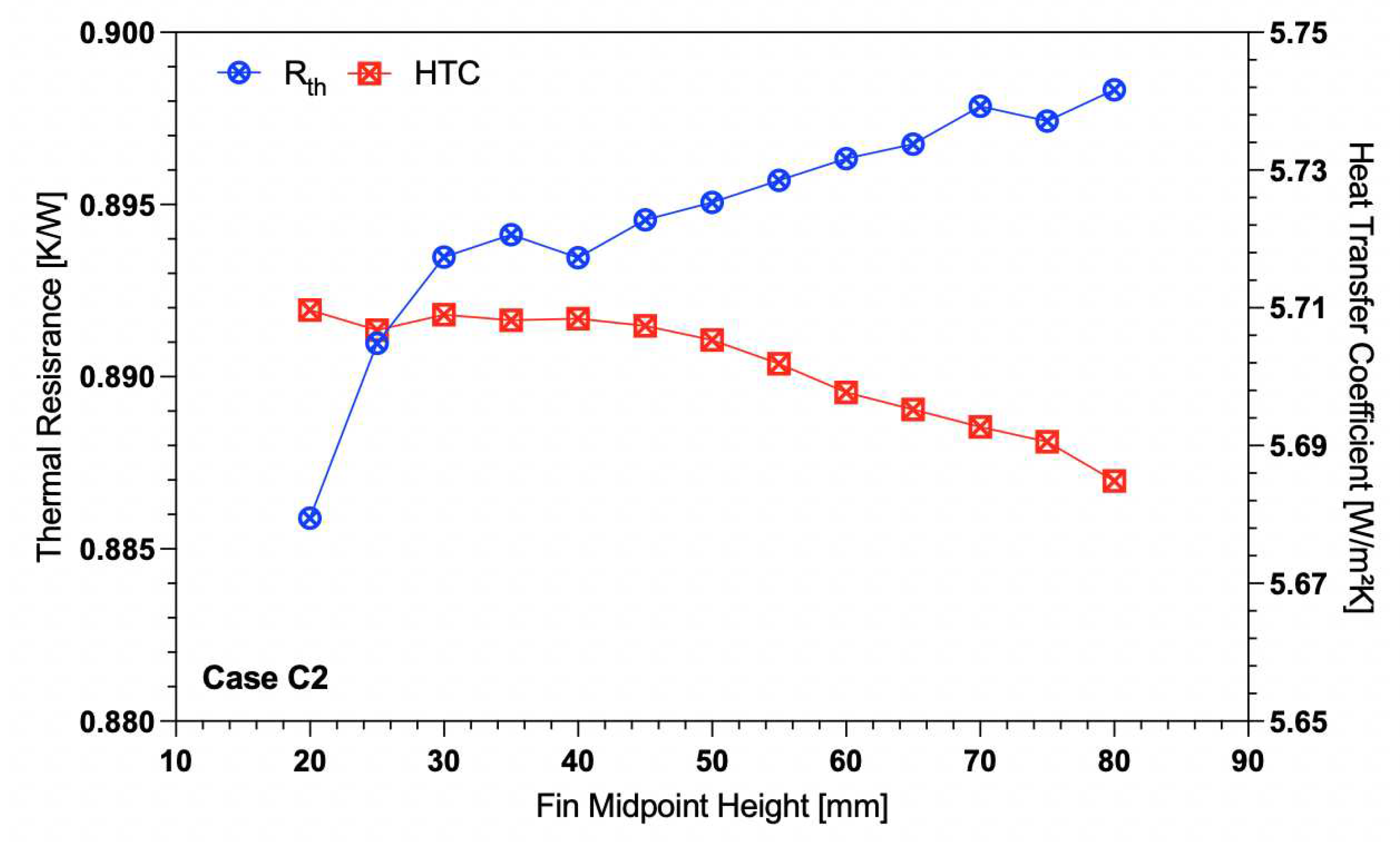
Figure 15.
Non-dimensional representation of performance parameters for all the design cases: (a) Thermal resistance, (b) Heat transfer coefficient, (c) Heat transfer coefficient by mass, and (d) Fin efficiency.
Figure 15.
Non-dimensional representation of performance parameters for all the design cases: (a) Thermal resistance, (b) Heat transfer coefficient, (c) Heat transfer coefficient by mass, and (d) Fin efficiency.
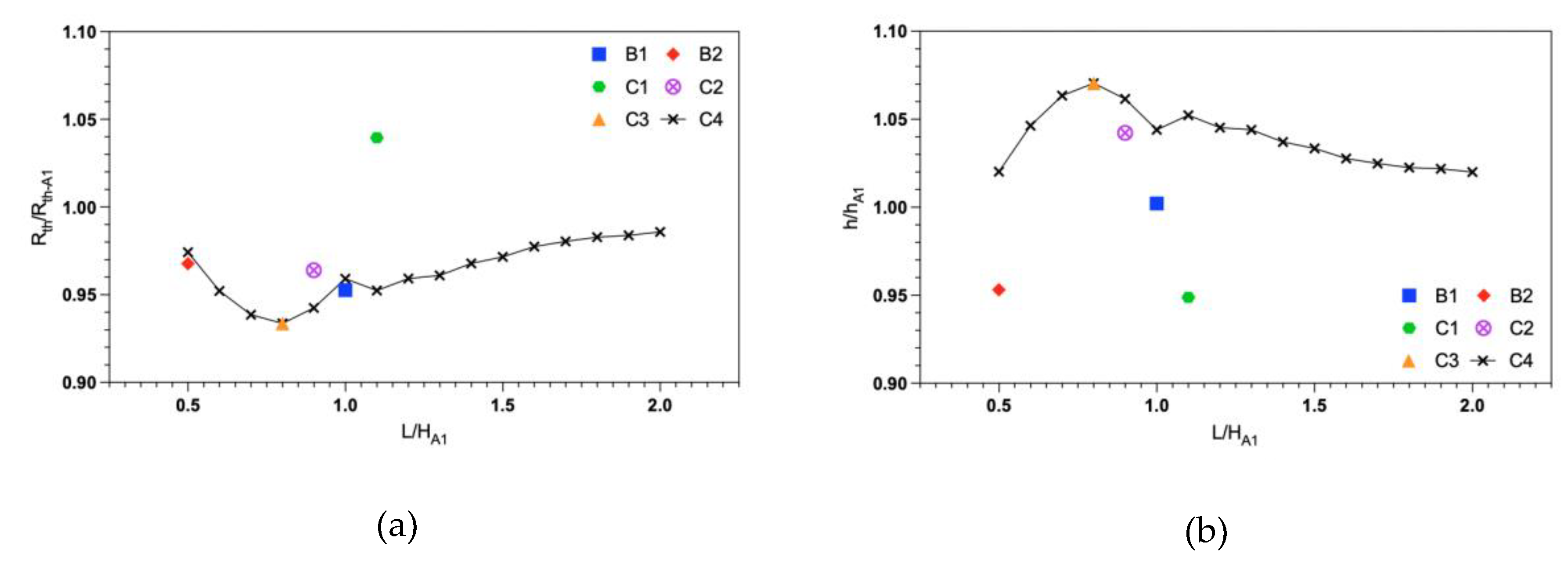
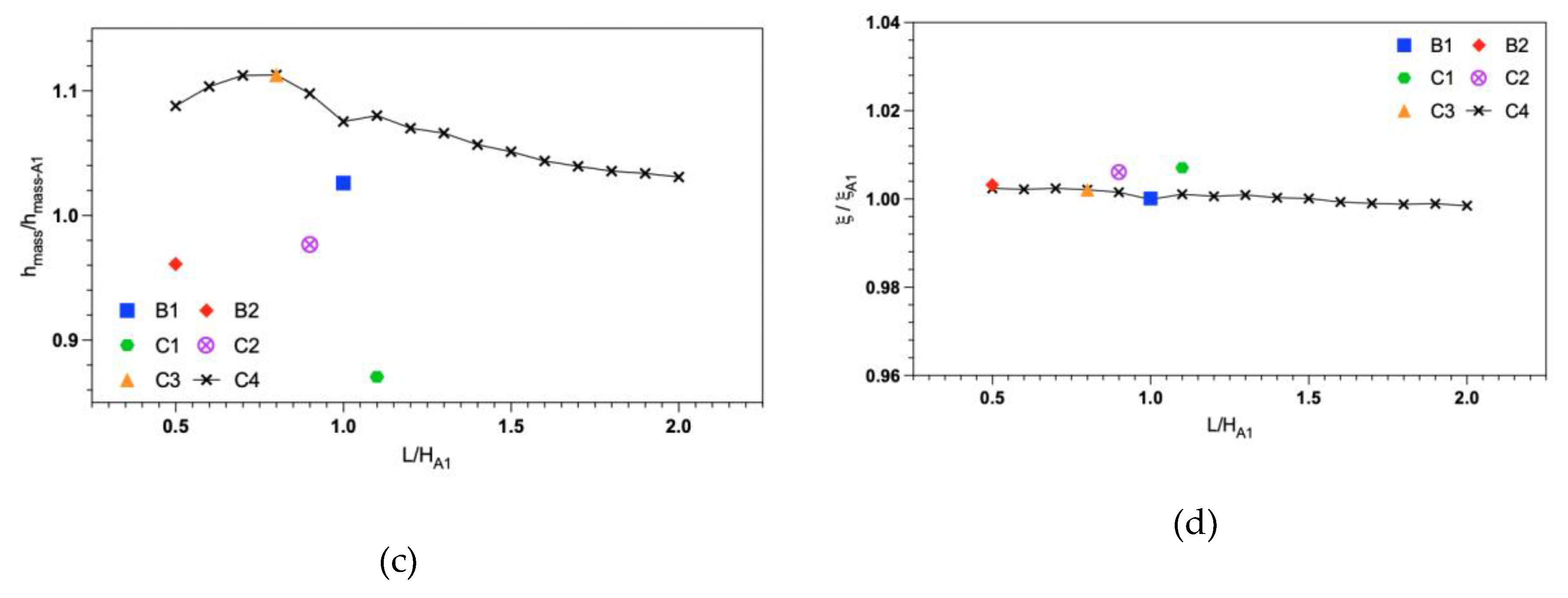

Table 1.
Fixed parameter values used in this CFD-based heat sink optimization study.
| Fixed Parameter | Value | Unit |
|---|---|---|
| Base Plate Height | 100 | mm |
| Base Plate Width | 100 | mm |
| Base Plate Thickness | 2 | mm |
| Fin Thickness | 2 | mm |
| Applied Heat Flux | 4000 | W/m2 |
Table 2.
Material properties for this CFD-based heat sink optimization study.
| Fixed Parameter | Unit | Aluminium alloy 2024 | Air |
|---|---|---|---|
| Density | kg/m3 | 2719 | 1.225 |
| Thermal conductivity | W/m.K | 202.4 | 0.0242 |
| Specific heat | J/kg.K | 871 | 1006.4 |
| Dynamic viscosity | kg/m.s | - | 1.789×10⁻⁵ |
| Thermal expansion coefficient | K−1 | - | 0.0033 |
Table 3.
Summary of the heat sink configurations studied.
| Design Code | Fin Shape | Parameter of Investigation | Range of Testing [mm] |
|---|---|---|---|
| A1 | Rectangular | Fin Spacing | 4 – 25 |
| A2 | Rectangular | Fin Length | 30 – 200 |
| B1 | Trapezoidal | Bottom Fin Length | 50 – 150 |
| B2 | Trapezoidal | Fin Length | 30 – 200 |
| C1 | Curved | Midpoint Length | 50 – 150 |
| C2 | Curved | Midpoint Height | 10 – 90 |
| C3 | Curved | Top Profile Length | 50 – 100 |
| C4 | Curved | Overall Fin Length | 30 – 200* |
| C5 | Curved | Fin Spacing | 4 – 25 |
| D1 | Angled | Symmetry on both sides and two different Fin Lengths | 55, 100 |
| D2 | Angled | Symmetry on one side and two different Fin Lengths | 55, 100 |
* Equivalent length of rectangular fin of equal area.
Table 4.
Angled fin design parameters.
| Parameter | Zhang et al. [3] | Present Study | Units |
|---|---|---|---|
| Vertical spacing | 8 | 8 | mm |
| Horizontal spacing | 6 | 6 | mm |
| Fin angle (to the horizontal) | 60 | 60 | Degrees |
| Fin length | 55 | 55 | mm |
| Base Plate width | 206 | 50 | mm |
| Base Plate height | 353 | 100 | mm |
| Fin thickness | 1.8 | 2 | mm |
Table 5.
Optimal fin spacing for a rectangular fin heat sink of length 100 mm.
| Geometry | Fin Spacing | Fin Number | Thermal Resistance (Rth) | Heat Transfer Coefficient (h) |
|---|---|---|---|---|
| Units | mm | - | K/W | W/m2K |
| Rectangular | 8.333 | 12 | 0.862 | 4.547 |
| Rectangular | 9.091 | 11 | 0.865 | 4.926 |
Table 6.
Summary of results using the laminar flow model without radiation. Relative differences are shown in [%] with respect to Case A1 (55 mm or 100 mm fin length, respectively).
Table 6.
Summary of results using the laminar flow model without radiation. Relative differences are shown in [%] with respect to Case A1 (55 mm or 100 mm fin length, respectively).
| DesignCase | FinLength | FinGeometry | Fin Max. Temp. | Avg. Vel. above Fins | HTC | ∆HTC | ||
|---|---|---|---|---|---|---|---|---|
| - | mm | - | K | m/s | K/W | % | W/m2K | % |
| A1 | 55 | Rectangular | 351.2 | 0.191 | 1.281 | 0.0% | 5.838 | 0.0% |
| D1 | 55 | Angled | 365.8 | 0.087 | 1.644 | +28.3% | 2.331 | -60.1% |
| D2 | 55 | Angled | 347.4 | 0.119 | 1.184 | -7.6% | 3.236 | -44.6% |
| A1 | 100 | Rectangular | 334.5 | 0.093 | 0.863 | 0.0% | 4.935 | 0.0% |
| D1 | 100 | Angled | 354.1 | 0.065 | 1.352 | +56.6% | 1.590 | -67.8% |
| D2 | 100 | Angled | 335.9 | 0.085 | 0.897 | +3.9% | 2.395 | -51.5% |
Table 7.
Summary of results using the laminar flow model with radiation enabled. Relative differences are shown in [%] with respect to Case A1 (55 mm or 100 mm fin length, respectively).
Table 7.
Summary of results using the laminar flow model with radiation enabled. Relative differences are shown in [%] with respect to Case A1 (55 mm or 100 mm fin length, respectively).
| DesignCase | FinLength | FinGeometry | Fin Max. Temp. | Avg. Vel. above Fins | HTC | ∆HTC | ||
|---|---|---|---|---|---|---|---|---|
| - | mm | - | K | m/s | K/W | % | W/m2K | % |
| A1 | 55 | Rectangular | 345.7 | 0.181 | 1.142 | 0.0% | 6.551 | 0.0% |
| D1 | 55 | Angled | 357.4 | 0.079 | 1.435 | +25.7% | 2.671 | -59.3% |
| D2 | 55 | Angled | 340.5 | 0.104 | 1.014 | -11.2% | 3.781 | -42.3% |
| A1 | 100 | Rectangular | 331.7 | 0.111 | 0.791 | 0.0% | 5.383 | 0.0% |
| D1 | 100 | Angled | 347.5 | 0.056 | 1.187 | +50.0% | 1.811 | -66.4% |
| D2 | 100 | Angled | 330.6 | 0.079 | 0.764 | -3.4% | 2.812 | -47.8% |
Table 8.
Summary of results using the transition-SST model with radiation disabled. Relative differences are shown in [%] with respect to Case A1 (55 mm or 100 mm fin length, respectively).
Table 8.
Summary of results using the transition-SST model with radiation disabled. Relative differences are shown in [%] with respect to Case A1 (55 mm or 100 mm fin length, respectively).
| DesignCase | FinLength | Fin Geometry | Fin Max.Temp. | Avg. Vel.above Fins | HTC | ∆HTC | ||
|---|---|---|---|---|---|---|---|---|
| - | mm | - | K | m/s | K/W | % | W/m2K | % |
| A1 | 55 | Rectangular | 341.2 | 0.205 | 1.030 | 0.0% | 7.264 | 0.0% |
| D1 | 55 | Angled | 346.9 | 0.084 | 1.172 | +13.8% | 3.270 | -55.0% |
| D2 | 55 | Angled | 343.1 | 0.104 | 1.078 | +4.7% | 3.556 | -51.0% |
| A1 | 100 | Rectangular | 329.5 | 0.213 | 0.738 | 0.0% | 5.776 | 0.0% |
| D1 | 100 | Angled | 343.3 | 0.002 | 1.081 | +47.0% | 1.988 | -65.6% |
| D2 | 100 | Angled | 330.7 | 0.057 | 0.766 | +3.9% | 2.805 | -51.4% |
Table 9.
Thermal performance of all the design cases with optimized fin spacing in terms of Rth and HTC. Relative differences are shown in [%] with respect to Case A1 (55 mm or 100 mm fin length, respectively).
Table 9.
Thermal performance of all the design cases with optimized fin spacing in terms of Rth and HTC. Relative differences are shown in [%] with respect to Case A1 (55 mm or 100 mm fin length, respectively).
| Design Case | FinLength | Array | FinTemp. | HTC | HTC(*) | HTC/Mass | HTC/Mass | |||
|---|---|---|---|---|---|---|---|---|---|---|
| mm | m2 | % | K | K/W | % | W/m2K | % | W/kgK | % | |
| A1 | 100 | 0.235 | 0.0% | 334.5 | 0.863 | 0.0% | 4.935 | 0.0% | 1.816 | 0.0% |
| B1 | 100 | 0.246 | 4.7% | 332.4 | 0.818 | -5.2% | 4.971 | 0.7% | 1.863 | 2.6% |
| B2 | 50 | 0.134 | -43.0% | 350.9 | 1.284 | 48.8% | 5.828 | 18.1% | 2.213 | 21.9% |
| C1 | 100 | 0.260 | 10.6% | 332.1 | 0.812 | -5.9% | 4.735 | -4.1% | 1.639 | -9.7% |
| C2 | 100 | 0.211 | -10.2% | 335.4 | 0.895 | 3.7% | 5.291 | 7.2% | 1.808 | -0.4% |
| C3 | 100 | 0.190 | -19.1% | 337.0 | 0.933 | 8.1% | 5.644 | 14.4% | 2.116 | 16.5% |
| C4 | 100 | 0.234 | -0.4% | 332.6 | 0.824 | -4.5% | 5.178 | 4.9% | 1.963 | 8.1% |
| D1 | 100 | 0.465 | 97.9% | 354.1 | 1.352 | 56.7% | 1.590 | -67.8% | 1.140 | -37.2% |
| D2 | 100 | 0.465 | 97.9% | 335.9 | 0.897 | 3.9% | 2.395 | -51.5% | 1.718 | -5.4% |
| A1 | 55 | 0.134 | 0.0% | 351.2 | 1.294 | 0.0% | 2.346 | 0.0% | 2.180 | 0.0% |
| D1 | 55 | 0.261 | 94.8% | 365.8 | 1.644 | 27.0% | 2.331 | -0.6% | 1.596 | -26.8% |
| D2 | 55 | 0.261 | 94.8% | 347.4 | 1.184 | -8.5% | 3.236 | 37.9% | 2.216 | 1.7% |
Disclaimer/Publisher’s Note: The statements, opinions and data contained in all publications are solely those of the individual author(s) and contributor(s) and not of MDPI and/or the editor(s). MDPI and/or the editor(s) disclaim responsibility for any injury to people or property resulting from any ideas, methods, instructions or products referred to in the content. |
© 2023 by the authors. Licensee MDPI, Basel, Switzerland. This article is an open access article distributed under the terms and conditions of the Creative Commons Attribution (CC BY) license (http://creativecommons.org/licenses/by/4.0/).
Copyright: This open access article is published under a Creative Commons CC BY 4.0 license, which permit the free download, distribution, and reuse, provided that the author and preprint are cited in any reuse.


