1. Introduction
Tactile sensors have gained immense popularity in robotics and automation systems in applications like artificial skins, etc. as they provide pressure maps through a force sensor array. However, hysteresis, a well-known phenomenon, can introduce nonlinearity and measurement errors in tactile sensors and actuator systems, limiting the performance of tactile sensors. To address this challenge, several novel approaches have been proposed in recent years. One approach focuses on adapting the external loop of the sensor's control system to compensate for hysteresis [
1]. By estimating the hysteresis error based on the difference between the desired and measured forces, this modification improves the accuracy and performance of robotic systems by relying on tactile sensors. In the field of piezoelectric actuators, one study introduced a method for modeling hysteresis patterns using a recurrent neural network (RNN) [
2]. This RNN captures the complex nonlinear relationship between the input voltage and output displacement, enabling hysteresis compensation and enhancing positioning system accuracy. Furthermore, a generalized Prandtl-Ishlinskii model has been employed to compensate for hysteresis in tactile sensors [
3]. By training the model with experimental data, real-time sensor output can be estimated, effectively improving force measurement accuracy. Additionally, innovative designs have been developed to minimize hysteresis in tactile sensors, such as a novel soft tactile electronic skin that reduces mechanical and electrical memory effects contributing to hysteresis [
4]. Similarly, a method utilizing a Gaussian process with sensory Markov properties has been proposed to counteract hysteresis in tactile sensors [
5]. By incorporating current and past sensory data, the current approach models the hysteresis behavior and estimates the sensor's output, improving force measurement accuracy in robotic systems. In the field of smart-material systems, an inverse feedforward controller utilizing a Preisach model has been introduced to control hysteresis nonlinearities [
6]. This method estimates the hysteresis behaviour and generates an inverse feedforward control signal to compensate for the nonlinearities, enhancing the performance and accuracy of smart-material systems. Furthermore, a Generalized Prandtl-Ishlinskii Model (GPIM) inversion technique proposed to compensate for hysteresis in micro positioning control systems [
7]. By modelling the hysteresis behaviour using a GPIM and generating an inverse GPIM-based compensation signal, we can improve the accuracy and performance of the micro positioning control system. In the field of piezoelectric actuators, a modified Prandtl-Ishlinskii (PI) model has been introduced to accurately capture the asymmetric hysteresis behaviour [
8]. Several studies have explored hysteresis compensation in soft sensors. For instance, a modified generalised Prandtl-Ishlinskii (GPI) model has been developed for modelling the asymmetric hysteresis nonlinearity of pneumatic artificial muscles (PAMs) [
9]. Additionally, a novel hysteresis model for piezoelectric actuators has been introduced, incorporating memory effects [
10]. Several recurrent neural networks have been used to mitigate hysteresis in soft sensors [
11], and an improved method for hysteresis modelling and correction in soft sensors has been proposed, utilizing a radial basis function neural network [
12]. Another adaptive method for hysteresis modelling and compensation in soft sensors employs a fuzzy neural network [
13]. Furthermore, an improved method for hysteresis compensation in soft sensors has been presented, utilizing a hybrid neural network [
14].
Significant progress had been made in the compensation and modelling techniques for hysteresis in soft sensors based on piezoresistive materials. However, practical and effective methods were needed to correct hysteresis nonlinearity. To address this issue, a novel approach was proposed that utilized a backpropagation neural network (BPNN). The BPNN was trained using input-output data pairs from experimental tests to modify the hysteresis nonlinearity in soft sensors. This approach aimed to enhance the accuracy of soft sensors and overcome the limitations posed by hysteresis.
For training the BPNN, the collected force sequences and their corresponding corrected resistances were used as inputs. The training process demonstrated favourable convergence and achieved a high level of accuracy. The effectiveness of this approach was validated through experiments, showing a significant reduction in the maximum error caused by hysteresis. The maximum error was reduced from 24.2% to 13.5% of the sensor's full-scale output.
2. Modelling the Hysteresis Nonlinearity of Conductive Fibre-Based Tactile Sensors using Backpropagation Neural Networks
Soft tactile sensors based on piezoresistive materials have drawn significant attention in recent years due to their wide-ranging applications in robotics, medical devices, consumer electronics, and gaming. However, the accuracy of these sensors is often hindered by hysteresis, a nonlinear phenomenon wherein the sensor's output is influenced by its current input and previous history. This hysteresis can introduce notable measurement errors and compromise the reliability of the sensor.
Several methods have been proposed to address this issue and modify the hysteresis nonlinearity of piezoresistive sensors, including curve-fitting models and neural network approaches [15-18]. Though hysteresis approximation using BPNN has been previously employed, the novelty of the proposed method lies in its specific application to a conductive fibre-based tactile sensor. A novel approach is introduced in the paper by employing BPNN to modify the hysteresis nonlinearity in this particular sensor type, which has not been explored in previous studies within the context of conductive fibre-based tactile sensors.
It should be emphasised that the novelty of a research contribution is not solely determined by the individual components or techniques utilised. Instead, it often resides in combining or applying these components in a new or unique context. In this instance, although using BPNN for hysteresis approximation is not groundbreaking, its application to conductive fibre-based tactile sensors represents a fresh approach within the specialised domain of tactile sensing.
The focus on conductive fibre-based tactile sensors in the present paper contributes to the existing knowledge by addressing the distinctive challenges and characteristics associated with this sensor type. By leveraging the capabilities of BPNN, the proposed method modifies the hysteresis nonlinearity, thereby augmenting the accuracy and performance of conductive fibre-based tactile sensors in force measurement and control applications.
In summary, although using BPNNs for hysteresis approximation is not new, the paper's contribution lies in applying this method to conductive fibre-based tactile sensors. This method addresses such sensor's specific challenges and requirements, thereby advancing the field of tactile sensing and offering new possibilities for improving force measurement and control in relevant applications.
The experimental setup used to design four distinct types of sensor units with varying layers is described, along with the process of collecting output resistances by applying force sequences. These force sequences and the corresponding corrected resistances are employed as inputs to train the BP-NN, resulting in favourable convergence and high accuracy (
Figure 1). Through validation experiments, we demonstrate that the proposed approach significantly reduces the maximum error caused by hysteresis, reducing it from 24.2% to 13.5% of the sensor's full-scale output.
Subsequent sections delve into the theoretical background underlying hysteresis modelling, curve-fitting models, and neural networks. Additionally, we elucidate how these methods are integrated into the proposed approach, showcasing a block diagram and a specific algorithm.
-
(a)
Hysteresis Model Using Neural Network:
The hysteresis model uses a BPNN that takes the input force sequence and outputs the corresponding output resistance. The neural network is trained on a set of input-output data pairs, where the input is the force sequence, and the output is the corresponding output resistance of the tactile sensor. During training, the neural network adjusts its weights to minimise the difference between predicted and actual output resistance. Once trained, the neural network can be used to predict the output resistance for any given force sequence [19-21].
-
(b)
Curve-Fitting Model(s)
Curve-fitting models analyse data points to establish relationships between variables, aiding in predictions and understanding patterns, with effectiveness depending on data quality and proper model selection. [
22,
23]. In this study, a polynomial curve-fitting model was used to correct the hysteresis nonlinearity of the tactile sensor. The polynomial curve-fitting model is given by following equation:
where R is the corrected output; F is the raw input, and a
0, a
1, and a
n are the polynomial coefficients. The coefficients are determined by minimising the sum of the square error between the corrected output and the actual output.
-
(c)
Neural Network
Neural networks (NN) are computational models that learn complex patterns and relationships from data. With their interconnected layers and mathematical operations, they enable accurate predictions and valuable insights in various domains. In this paper, a BPNN was employed to modify the hysteresis nonlinearity of the tactile sensor.[
24]
The BPNN algorithm consists of two phases: forward and backward. In the forward phase, the input is propagated through the network to generate the output. In the backward phase, the error between the actual output and the desired output is propagated backward through the network to adjust the weights of the nodes. [
25,
26] The algorithm can be summarised as shown below:
Here represents the output of node j in layer l; is the weight connecting node I in layer l-1 to node j in layer l; is the output of node I in the previous layer’; is the bias of node j in layer l; and is the activation function.
In the backward phase, the error between the actual output and the desired output is propagated backward through the network to adjust the weights of the nodes. The error
each node j in layer l measures how much that node contributes to the overall network error. It is defined as the partial derivative of the total error E for the input
of node j in layer l.
The weight updates are then determined based on this network error. The weights are adjusted in a direction that reduces the error by an amount proportional to the error and the previous layer's output. This is known as the delta rule:
Here
is the learning rate, which controls the size of weight updates. The biases are updated similarly:
These weight and bias updates are applied to the network after each input is processed to reduce the error gradually over time. By iteratively adjusting the weights and biases, the network can learn the mapping between the input and the desired output.
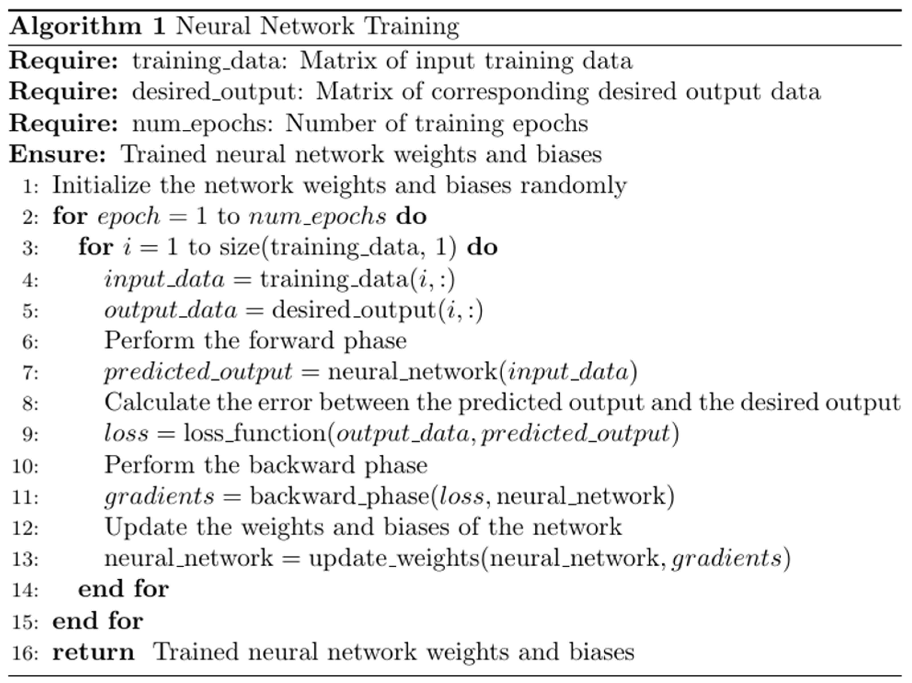
The algorithm can be summarised as follows:
Initialise the weights and biases of the network randomly.
-
For each input in the training data:
Perform the forward phase to generate the output of the network.
Calculate the error between the actual output and the desired output.
Perform the backward phase to adjust the weights of the network. Calculate the error between the actual output and the desired output.
Repeat step 2 for a specified number of epochs or until the network reaches a satisfactory level of performance. (see Algorithm 1)
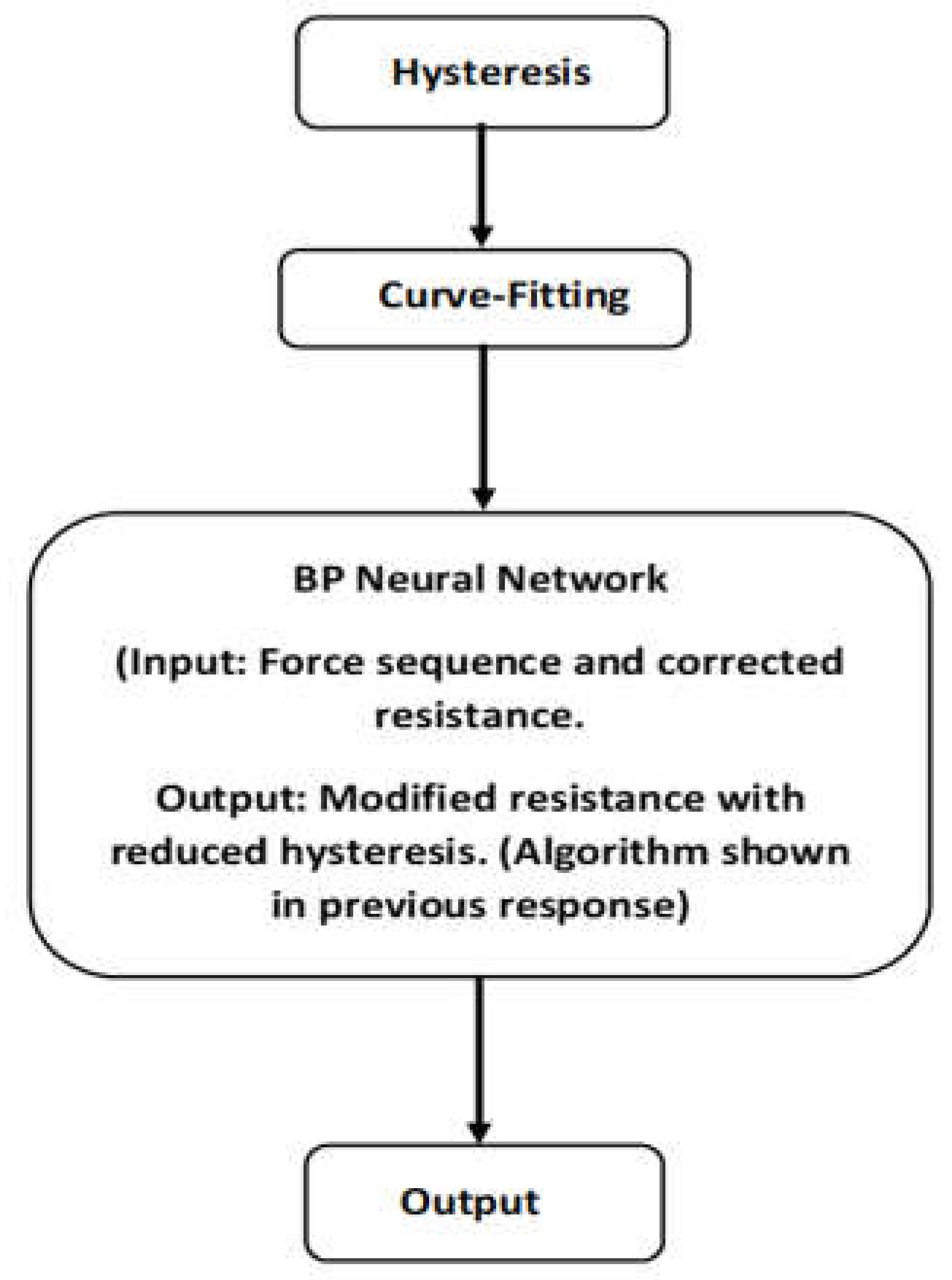
Here is a generic block diagram showing the integration of the hysteresis model, curve-fitting model, and BPNN (
Figure 2):
The integration of the hysteresis model, curve-fitting model, and BPNN provides a comprehensive approach for modelling a system where force is the input and resistance is the output. The hysteresis model captures the non-linear dynamics and memory effects of the system in response to force. The curve-fitting model approximates the mathematical relationship existing between force and resistance. The BPNN learns from the curve-fitting model's output to improve resistance predictions using backpropagation. This integrated system takes force as input, processes it through the hysteresis model, refines the output with the curve-fitting model, and further enhances it with the BPNN, thereby generating accurate predictions of resistance based on the force applied.
3. Design a Soft Tactile Sensor
Fabric-based sensors are selected due to their simple design, ease of fabrication, and low cost. They are stretchable and flexible and can adhere to soft surfaces. In the following section, the fabrication and design of the tactile sensor are discussed.
3.1. Use of Materials
The fabric sensor used in this study operates based on the piezoresistive effect, which induces a decrease in the electrical resistance of a piezoresistive material upon applying pressure. The sensor consists of two main components:
These materials work synergistically to create a tactile sensor that detects and converts pressure changes into analogue electrical signals, typically in voltage.
3.2. Sensor Assembly
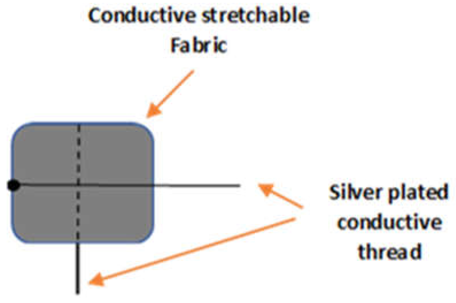
Assembling the sensor involved integrating the tactile sensor fabric with textiles to enable measurements of muscle activities. The silver-coated conductive thread was utilized to connect the sensor to a measurement system. This 100% polyamide fully silver-plated thread, with a linear resistance of <300 Ohm/m, was chosen for its low resistance characteristics. In this study, the silver-plated thread was employed to optimize contact points and circuit paths [30, 31]. The data for resistance versus force relationship was collected manually and saved in an Excel file. MATLAB program was utilised for data analysis and for generating plots to visualise the relationship between resistance and force (
Figure 3).
Figure 3(a) displays the EeonTexTM knitted conductive fabric, which contains conductive fibres that allow electrical current to flow through it. This fabric is used in various applications, such as smart textiles, wearable technology, and sensor systems.
Figure 3(b) displays the silver-plated thread, a conductive thread made by coating a base thread with a layer of silver. This thread is often used with conductive fabrics to create wearable electronics and others. Lastly,
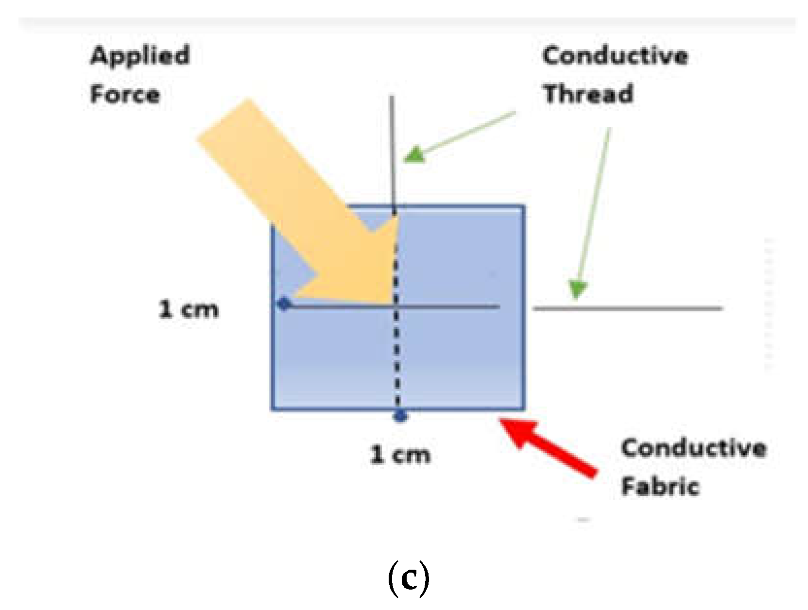
Figure 3(c) shows the complete sensor design that utilises the EeonTexTM knitted conductive fabric and silver-plated thread. The specific design of the sensor is for detecting the electric resistance signals when applying forces.
To keep the elasticity of the fabrics, the thread was sewn using a long-running loose stitch (saddle stitch). All the necessary pieces of samples were prepared with dimensions of 1 × 1 cm
2.
Figure 4 shows the overall diagram of the designed soft tactile sensor.
3.3. Experimental Setup
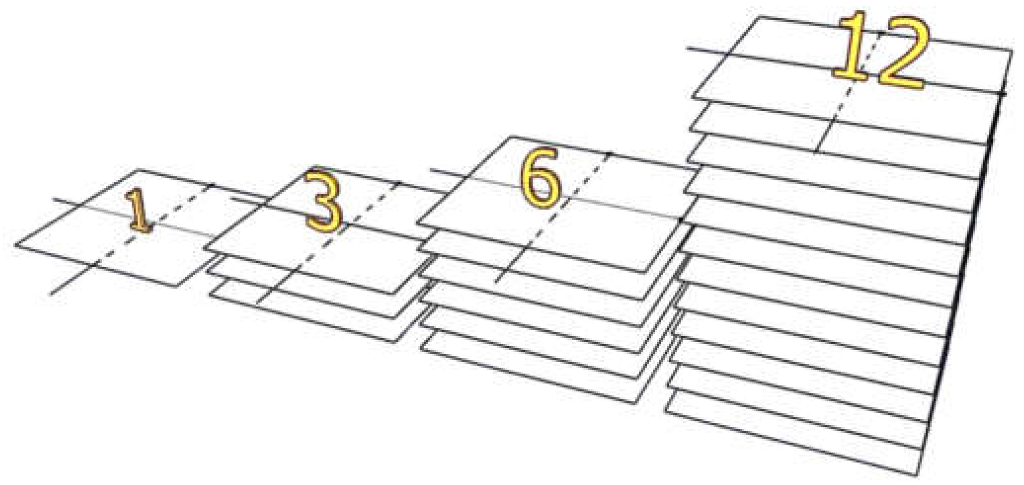
In the current study, we used four tactile sensor samples (one, three, six, and twelve layers) see
Figure 5. We designed the sensor in layers three, six, and twelve to increase the range of applying force to be measured. An increase in the number of layers implies an increase in the capacity of the tactile sensor to apply force, and it can be used in other applications, such as in the patient's seat or bed.
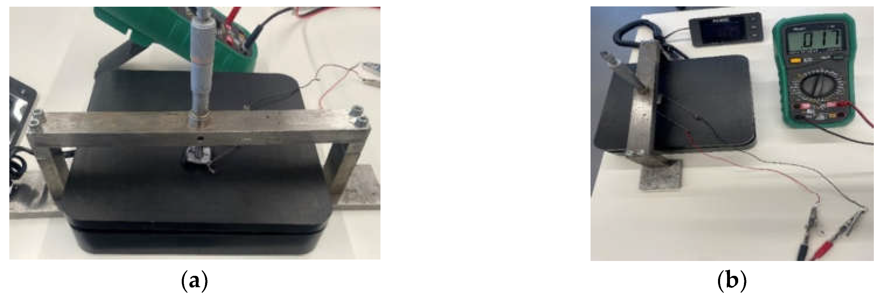
For each sensor, we applied forces using a force instrument that stands over the sensor, which is installed on the digital electronic weight scale (
Figure 6), after which the change in resistance is measured via a multi-meter.
Figure 6(a) shows the placement of a sensor on a weight scale when force is applied using a force instrument. It depicts the sensor's location of the object being weighed or the type of force instrument being used.
Figure 6(b) shows a setup for measuring the resistance change of a tactile sensor. Finally,
Figure 6 (c) shows a functional diagram or schematic of how to apply force to a tactile sensor. This involves using a specific mechanism to exert pressure or tension on the sensor in a controlled manner.
To study the behaviour of the tactile sensor output, a measurement method was used to register the sensor response to the sequences of forces that are exerted manually. Four to six consecutive loading-unloading cycles with different points of return for the same ascending curve and different starting points rising from the same descending curve are applied. Thus, the descending and ascending behaviour of the sensor is respectively characterised. The cycles are performed with an increase of 0.1 N between forces. These hysteresis curves represent the average output produced by the tactile sensor point after repeating each cycle five times. The interval between the new force level being exerted and the resistance output is 2 sec. To quantify the hysteresis exhibited by the sensor, the hysteresis error as the difference in sensor output resistance to the same applied force is determined when these forces are exerted on the ascending and descending branches of cycles. The maximum force applied by using a force instrument to the tactile sensor varied depending on the type of object used to apply force. When using the index fingertip on a thin ring, the maximum force (F) was 59.5±21.4 N, while when using all four fingers on a straight bar, the maximum force (F) was 268.7±77.2 N [
32]. This variation in the F values reflects the different force ranges that the sensor is expected to encounter in real-world applications and provides essential data for understanding the sensor's response to different levels of force.
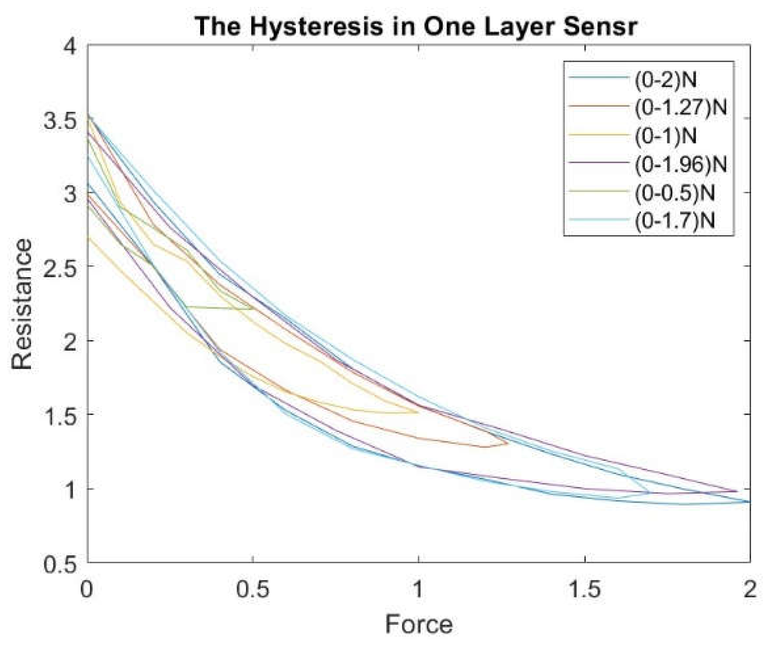
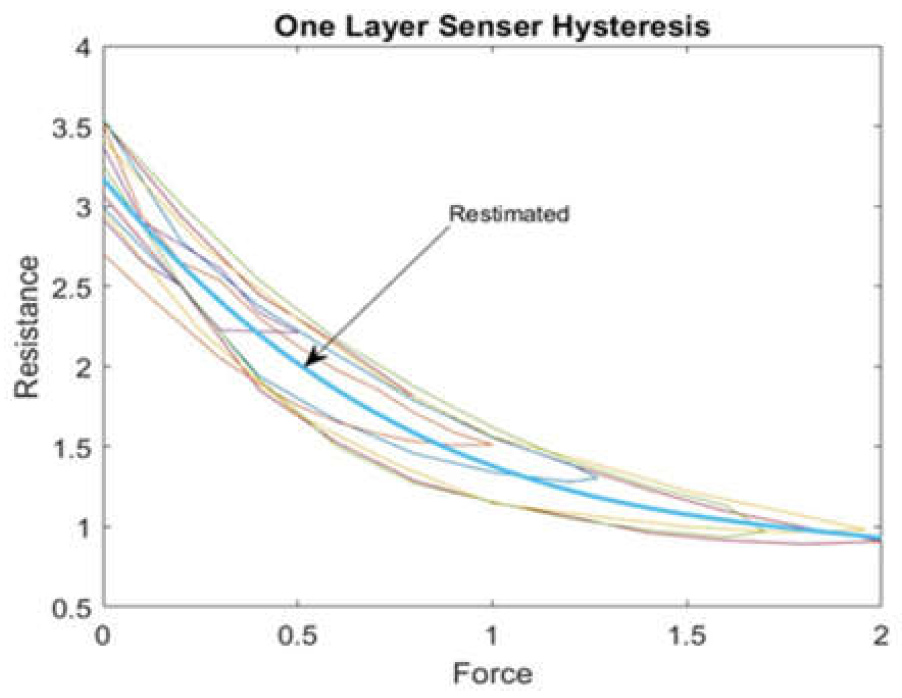
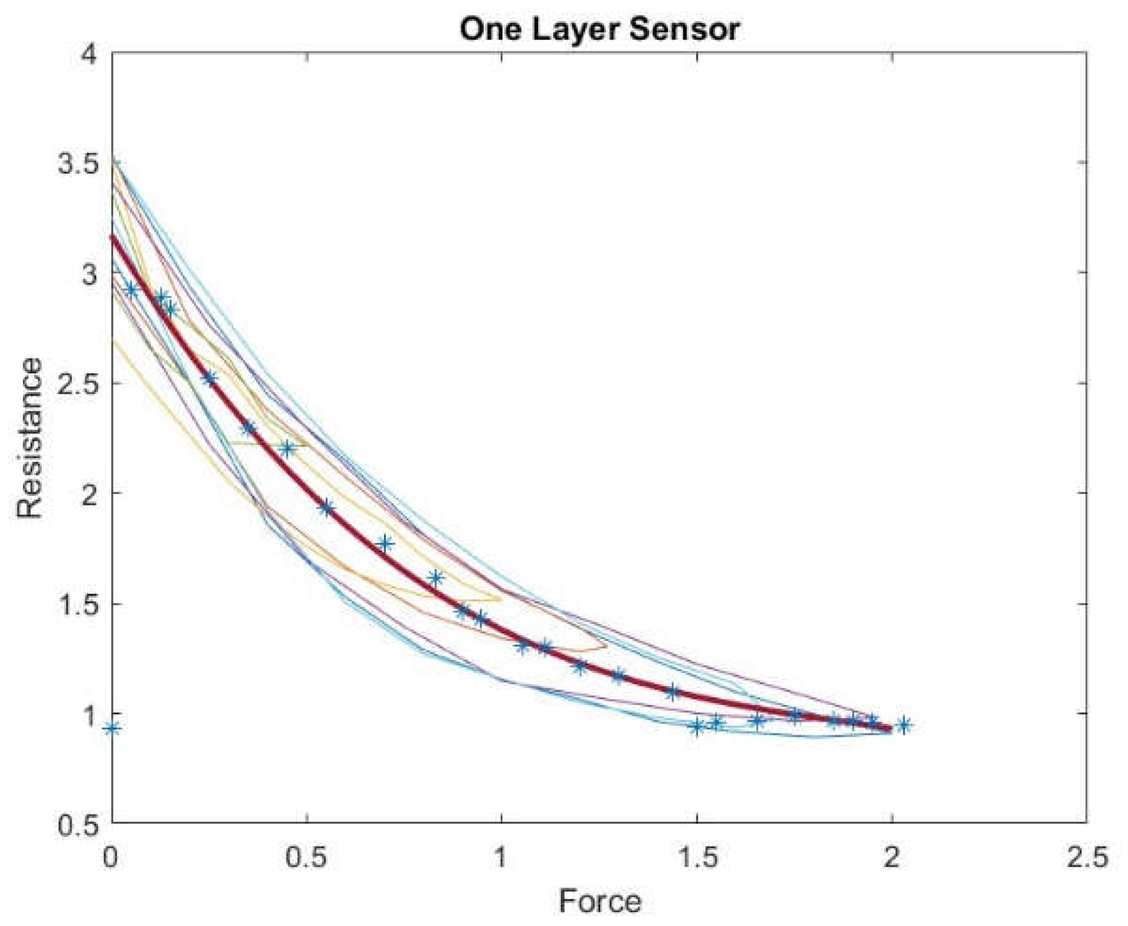
For the one-layer sensor, we applied a force of more than 0-2 N; the load was increased until the sensor output reached its saturation level. Then, we reduced the load from 2 to 0 N and measured the resistance change; accordingly, we plotted the results as a force function. We repeated this experiment with random force ranges (0-1.27 N, 0-1 N, 0-1.96 N, 0-0.5 N, and 0-1.7 N).
Figure 7 shows the hysteresis in the one-layer sensor.
The maximum and average hysteresis errors are referenced to the highest output value to obtain a percentage of the error relative to the full scale. The maximum error due to hysteresis is 24.2% of full-scale output.
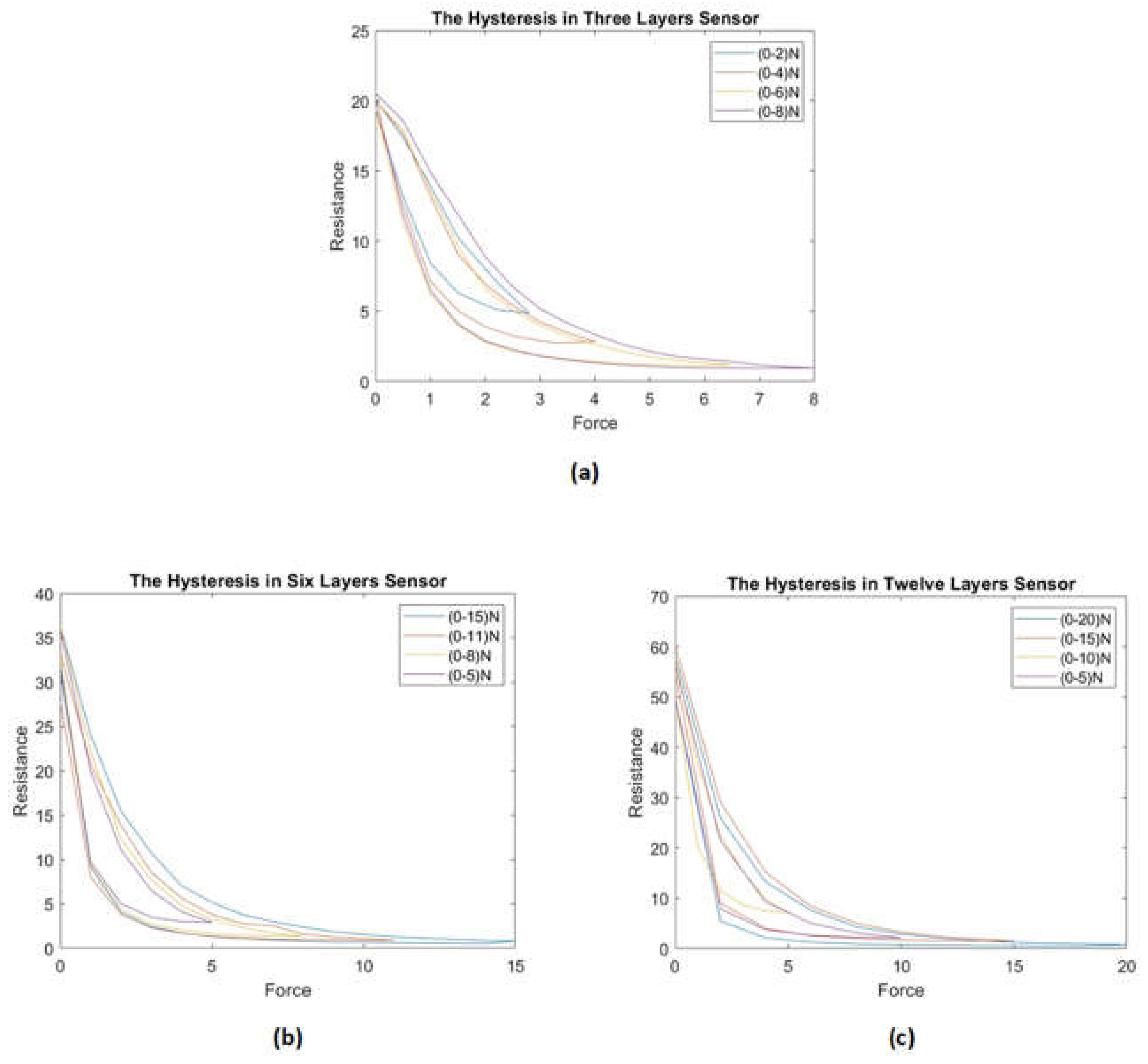
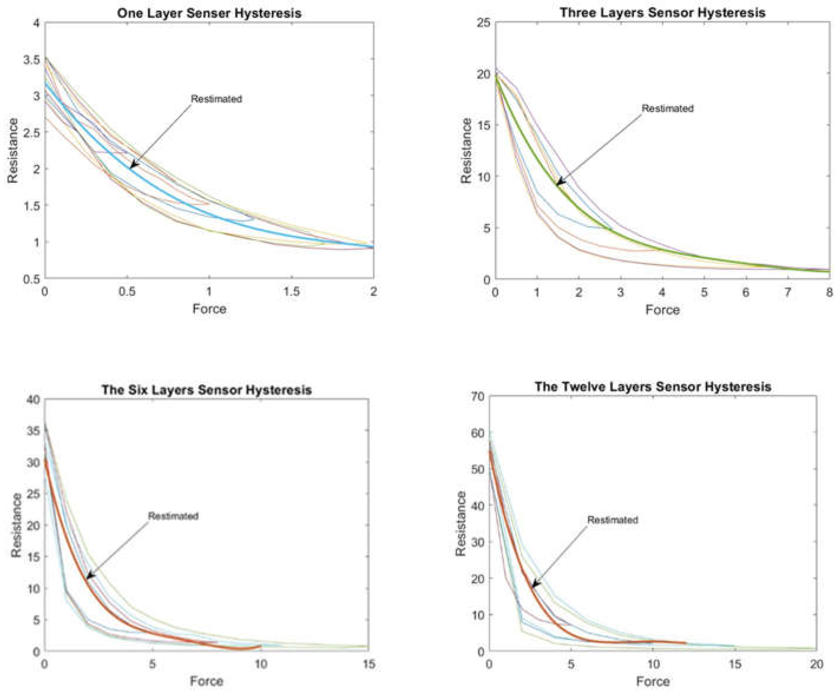
For the three-layer sensor, we applied force ranges of 0-2.8 N, 0-4 N, 0-6 N, and 0-8 N and recorded the associated resistance changes over several experiments, reporting the average resistance over the individual experiments as a function of force.
The experiment was again repeated with the six- and twelve-layer sensors and the associated hysteresis was plotted accordingly.
Figure 8 shows the hysteresis for the three-, six- and twelve-layer sensors.
Figures (7) and (8) illustrate that the hysteresis curve of the proposed sensor exhibits a multi-loop behaviour in different layers of the sensor. This means that the output resistance of the sensor depends not only on the current force applied but also on the force history.
Figure (7) shows the hysteresis behaviour of the sensor when it is compressed to a maximum force and then released multiple times. The sensor exhibits a different number of loops, indicating that the sensor's hysteresis behaviour varies depending on the sensor's compressed and released layer. The number of loops increases as compressions and releases increase, indicating that the force history influences the sensor's hysteresis behaviour. Similarly, Figure (8) shows the hysteresis behaviour of the sensor when it is compressed and released multiple times in the same layer.
The findings emphasize that the output curve of the proposed sensor is influenced by both the current force applied and the force history. This underscores the significance of considering the hysteresis phenomenon during the design and interpretation of results from tactile sensors. To tackle this challenge, the paper proposes a Backpropagation Neural Network (BPNN) that adjusts the sensor's resistance based on estimated values obtained from the polynomial curve. This approach enhances the accuracy and reliability of readings, enabling more precise interpretations of the sensor's output.
4. Modelling Hysteresis Based on Backpropagation Neural Network
Neural networks are a popular choice for compensating for hysteresis in tactile sensors because they can effectively learn the complex nonlinear relationships between input and output data.
Tactile sensors are used to detect and measure physical forces, pressures, and vibrations, among other things. Hysteresis is a common problem encountered in tactile sensors that can cause measurement inaccuracies. Hysteresis occurs when the sensor's output does not return to its original state after the input has changed, causing a lag in the sensor's response. [30-32]
Neural networks can learn to compensate for this hysteresis by analysing the sensor's input-output data and building a model to predict the correct output based on the input. They can learn the nonlinear relationship between input and output data, allowing them to compensate for hysteresis accurately. [
33]
Though other methods can also be used to compensate for hysteresis in tactile sensors, such as physical calibration or mathematical modelling, these methods may be less effective in capturing the complex nonlinear relationship between input and output data. Neural networks offer a flexible and powerful solution for hysteresis compensation in tactile sensors. [
34]
Nonlinear hysteresis in a tactile sensor can result in degraded system performance and instability [
35]. In the experiment, a BPNN was used to eliminate nonlinear hysteresis as an Artificial Neural Network (ANN) is simple and sufficient for the problem we discussed, albeit within the tactile sensor. BPNNs have a high precision approximation, robust fault tolerance, and nonlinear solid mapping capabilities [35-37].
A Back Propagation (BP) neural network was used due to its better generalisation and strong nonlinear mapping abilities, which make it a popular choice in various fields. The BPNN was trained to predict the static resistance value based on the current and historical resistance values (R
at and R
t-1 respectively) and the estimated resistance value, which was used as a target [
38,
39,
40].
The neural network used in the study consisted of an input layer that has the current resistance R
t at a time(
t), the historical resistance R
t-1 at a time (
t-1), and a corrected resistance (R
estimated) as a target, the output layer is a static resistance R
Statict for training, and two hidden layers. Each hidden layer has five neurons; the transfer function is the sigmoid function. The Levenberg-Marquardt algorithm (LMA) is a popular optimisation method for training neural networks. It is a variation of the Gauss-Newton algorithm which is known for fast convergence and good stability. Using the LMA algorithm to train the BPNN, the model could learn the complex relationships between the input and output variables and make accurate predictions [
41].
Overall, the use of BPNN in the proposed sensor system offers more accuracy and reliability, and different neural network techniques can be helpful in various applications where precise and consist of measurements are required.
5. Modified Hysteresis: Simulation and Experiments
A tactile sensor is used to verify the hysteresis model based on BP neural networks. The target part is determined by approximating a curve from the hysteresis graph, and for each layer, the approximated curve's line is plotted as a desired resistance.
Figure 9 shows the approximated curve plotted for one-layer sensor. This curve likely represents the relationship between the sensor's actual resistance values with the desired values represented by the curve; we can evaluate the accuracy of the hysteresis model and make any necessary adjustments.
A third–degree polynomial was used to fit the hysteresis curve in a one-layer tactile sensor, which provided the best practical results. After fitting the polynomial curve, the force values were substituted into the polynomial to determine the corresponding estimated resistance values. These estimated resistance values were then used as the target input for the BPNN.
BP is a popular neural network training algorithm used to adjust the network weights and to minimise the difference between the predicted and actual values [
42]. In this case, the target input was the estimated resistance value obtained from the polynomial regression, and the neural network was trained to predict this value based on the input force values.
The proposed model could capture the nonlinear relationship between the force and resistance values by combining the polynomial regression and neural network techniques and make accurate predictions. This approach can be helpful in various applications where complex relationships between variables are challenging to model using traditional techniques.
Fitting a polynomial curve to hysteresis data is a common approach, but it has limitations as the relationship is complex. In such cases, neural networks excel by capturing nonlinear patterns, extracting hidden features, generalising to new data, and handling diverse inputs. Their flexibility and ability to model complex relationships make neural networks a preferred choice when traditional methods struggle in machine learning [
23].
Once a polynomial curve is fitted to the hysteresis data, the estimated values can be used as inputs for a neural network. Neural networks are powerful machine learning models that can learn complex patterns and relationships in data. By using the estimated values from the polynomial curve as inputs for the neural network, the variables can make better predictions.
where F represents the force applied (0 – 2 N).
Equation (6) shows that the estimated value of R relates to the force applied (F) in the current study. The range of values for F in this equation is between 0 and 2N; 41 samples have been used to derive this equation.
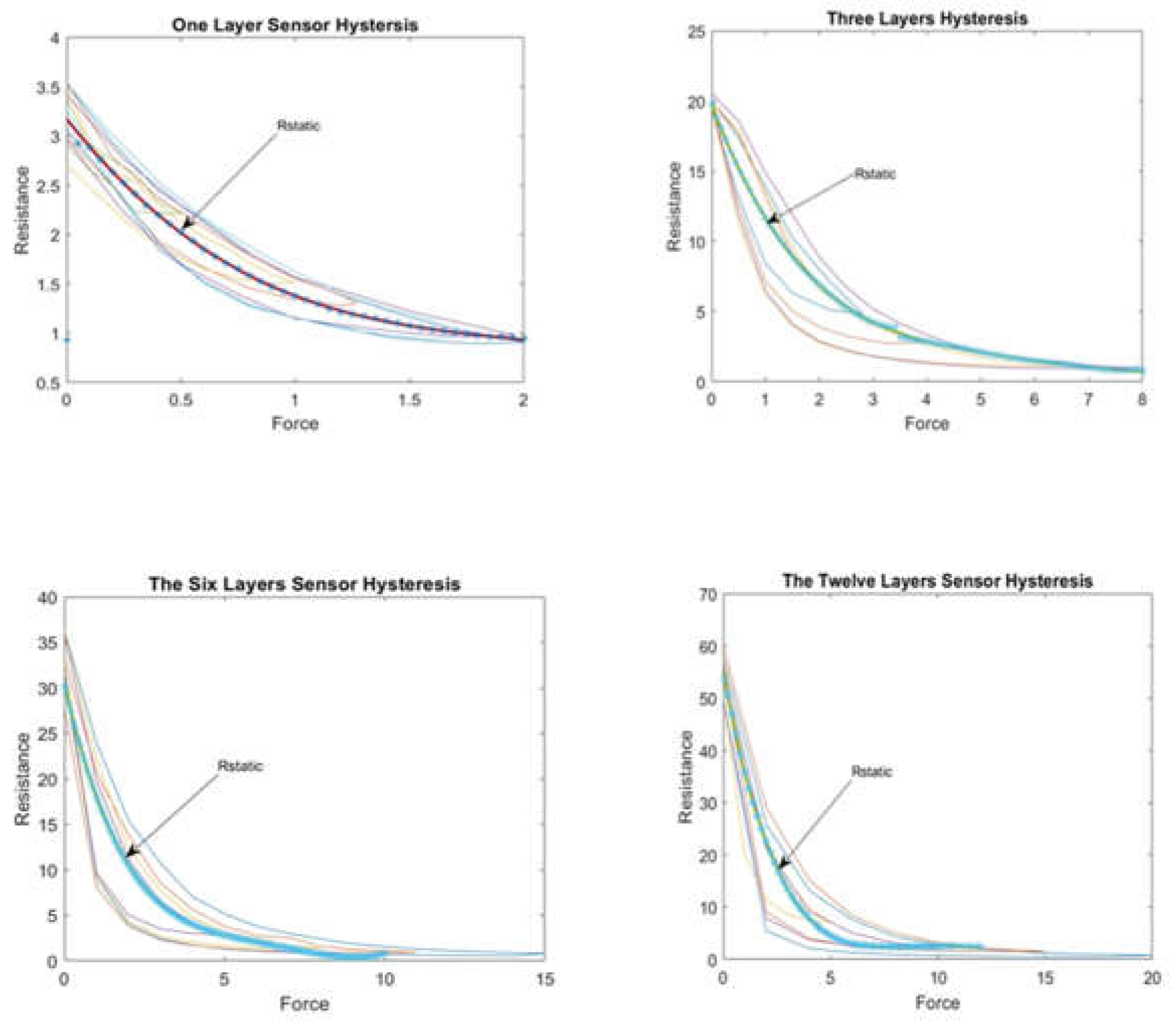
The earlier tested procedure of one layer sensor was repeated for all layers, with
Figure 10 showing the subsequent results:
The corrected curve equation for all layers of sensors can be found in the graphs shown above, and by using the same procedure of layer one sensor the desired target in our BPNN can be found.
The range of values for F in equation (7) is between 0 and 8N, and 90 samples are used to derive this equation.
Values for F in equation (8) range from 0 N to 15 N. Overall, 142 samples were used to derive this equation.
The range of values for F in this equation is between 0 and 20 N, and 240 samples have been used to derive this equation. Three equations 2- 4 represent the estimated curve equation for the three-, six-, and twelve-layer sensors.
The equations provide an estimate of the value of R (representing a dependent variable) based on the force (F) applied, an independent variable. Each equation exhibits different characteristics in terms of the power of F and the sign of the coefficients. This helps us understand the relationship between F and R.
The power of F in the equations captures complex and nonlinear relationships between F and R, accommodating different curves and intricate patterns. By considering powers of F ranging from 2 to 4, these equations can capture the nonlinearity and complexity present in the relationship between F and R. Positive coefficients indicate a direct relationship, while negative coefficients suggest an inverse relationship. These coefficients are determined through regression analysis and depend on the dataset and the statistical method employed.
6. The Sensitivity of the System
Uncertainty analysis is used to quantify the uncertainty in the output of a mathematical model by examining the uncertainty in its input [
43]. Uncertainty analysis aims to understand how much of the uncertainty in the output can be attributed to uncertainty in each input variable. This is important because it allows us to identify the most critical source of uncertainty and focus on reducing it. [
44,
45]
The analysis aims to conduct a sensitivity analysis using Monte Carlo simulation and understand the relationship between the force variable (F) and the estimated values of (R). This analysis is crucial for understanding the behaviour of the models and evaluating the impact of force on the estimated values.
Monte Carlo simulation was employed as a powerful tool to assess the sensitivity of the estimated values to different levels of applied force. The value of F was systematically varied within specified ranges to conduct the sensitivity analysis. The corresponding changes in the estimated (R) values were observed and analysed.
The analysis revealed significant findings regarding the relationship between the force variable and the estimated values of R. It provided insights into how changes in force affect the estimated resistance values. By systematically varying the force variable, we observed how the estimated values of R responded, enabling a comprehensive assessment of the models' behaviour.
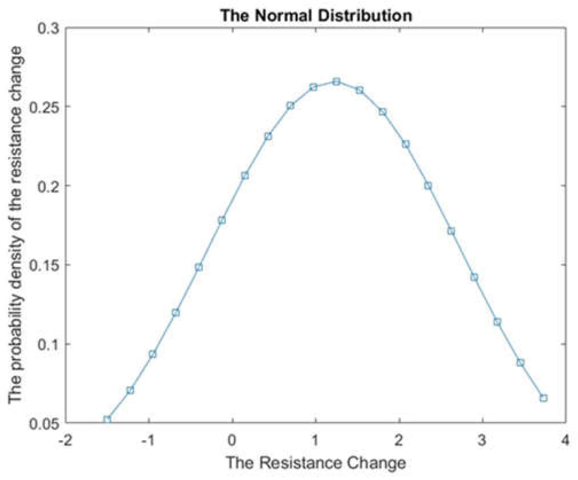
Figure 11 presents a normal distribution graph, which plays a crucial role in analysing and predicting data. The graph shows the distribution of the resistance variable within a population. The curve illustrates that the majority of values cluster around the mean, representing the centre or average value. As we move further away from the mean in both directions, the number of values gradually decreases.
In this specific case, the estimated mean distribution for the R-value was found to be 1.1125. This value serves as a measure of central tendency, indicating the average resistance value in the population. Additionally, the standard deviation of 1.513 indicates the spread or variability of resistance values from the mean.
By analysing the normal distribution graph and considering the mean and standard deviation, we gain valuable insights into the overall pattern and variability of resistance values.
7. Analysis and Discussions
The validation for the tactile sensor was performed by applying force and removing it from the sensors and measuring the corresponding changes in resistance. The observed resistance changes were then compared to the theoretically expected resistance changes. This validation process specifically focused on evaluating the performance and accuracy of the tactile sensor itself.
Figure 12 shows the validation of the system by using the same force data set as was used initially to train in the NN model for one-layer and other sensors.
As shown in
Figure 12, the tactile sensor has been specifically designed to accurately measure changes in resistance in response to applied or removed force. Through the validation process, the tactile sensor has demonstrated its capability to produce reliable and accurate results within the maximum force domain of 2 N for the layer one sensor.
The validation results indicate that the tactile sensor consistently provides measurements that closely align with the actual values of measurements. This alignment signifies that the predicted results generated by the neural network closely match the expected values based on the training data. Notably, the output results of the BP neural network, which fall perfectly on the target curve 'Restimated' after training, serve as a good indicator of the accuracy and reliability of the tactile sensor.
Furthermore, use of the same dataset for training and validation purposes facilitates a direct comparison between the predicted and actual results. When the predicted results closely resemble the actual results, the accuracy and reliability of the tactile sensor are confirmed in measuring resistance changes.
Based on these findings, we conclude that the tactile sensor is reliable and accurate in its measurements. It consistently provides highly dependable results and demonstrates high alignment between predicted and actual values. Accurately capturing resistance changes, reliable performance within the specified force range, and close alignment with actual results validate the reliability and accuracy of the tactile sensor in measuring resistance changes.
It may be highlighted that using the same data set for training and validation can potentially lead to overfitting, where the model becomes highly specialized to the training data and may struggle to generalise to new data. To address this concern, the model was validated using new and independent data sets also. The tactile sensor was tested with new sets of 25, 30, and 60 random forces, and the resulting output resistance was recorded and compared to the expected values (
Figure 13). This type of testing ensures that the model can accurately predict resistance values even when presented with new and previously unseen data.
Close alignment of the output results of the BP neural network with the target curve Restimated after training is a positive indication of the effectiveness of the training process. It suggests that the neural network has learned the underlying patterns and relationships between force and resistance, resulting in accurate predictions. This alignment between the predicted results and the target curve indicates that the neural network, and subsequently the tactile sensor, is performing well in accurately estimating resistance values.
Continuing testing and validation are essential to ensure the ongoing accuracy and reliability of the tactile sensor. This includes testing the tactile sensor under various conditions and using different data sets that were not included in the training process of the BPNN, to ensure its ability to generalize to new situations and data.
In addition to assessing the performance and accuracy of the BPNN, it is crucial to evaluate the robustness of the tactile sensor. Robustness refers to the ability of a sensor to maintain its performance and reliability despite uncertainties or variations in the input.
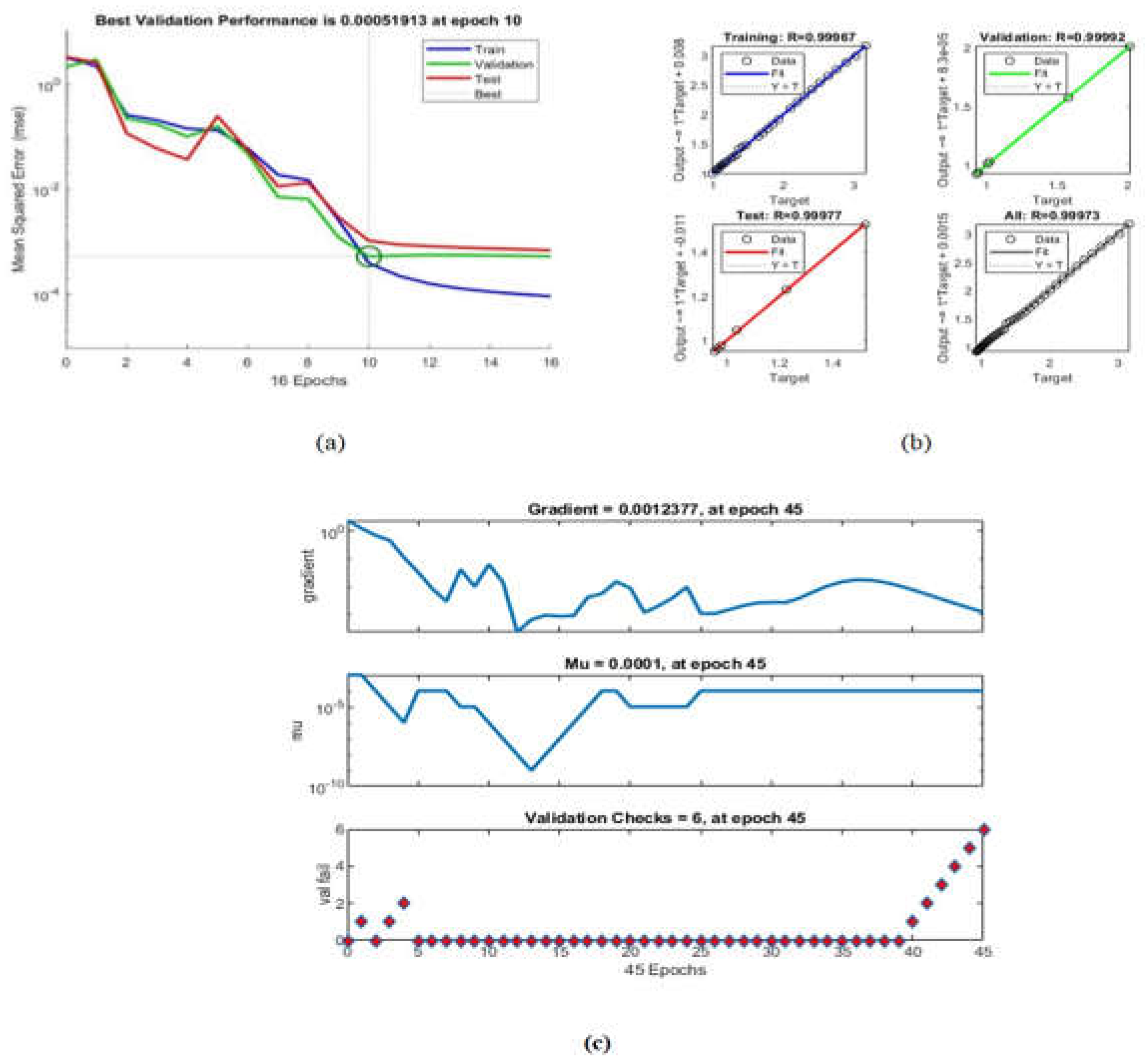
To evaluate the robustness of the tactile sensor, various factors, including the gradient, mu, and validation check values were considered for neural network training. Analysis revealed that at epoch 45, the gradient was 0.0012377, mu was 0.0001, and the validation check value was 6. These values provide insights into the stability and adaptability of the neural network during the training process.
Furthermore, the validation performance of the BPNN, as shown in
Figure 14(a), indicates the system's ability to maintain a low validation error of 0.000051913 at a specific epoch. This suggests that the neural network can consistently provide accurate predictions of the tactile sensor's resistance despite potential variations in the input force.
Data shown in
Figure 14(b) and the regression values shown in
Table 1 reveal that the system exhibits remarkable robustness. The high R-values across all datasets (training, validation, test, and overall) indicate a strong correlation between the predicted resistance values and the actual values. This consistency in performance demonstrates the system's ability to handle variations in input effectively.
Moreover, utilising a new dataset for validation, distinct from the one used for training, provides an additional measure of the system's robustness. By evaluating the system's performance on unseen data, the generalisability and ability of the system to handle new scenarios can be evaluated. The close alignment between the predicted and the actual results on the validation dataset suggests that the system maintains its accuracy and reliability when faced with new inputs.
Overall, the system's robustness is the combination of a low validation error, high correlation coefficients, stability during training, and consistent performance on new datasets. These findings highlight the system's ability to reliably measure changes in resistance based on the applied force, even in the presence of uncertainties or variations in the input. The system's robustness enhances its practical utility and strengthens its potential for various applications.
By conducting a comprehensive analysis of the system's performance, accuracy, and robustness, we gain valuable insights into its behaviour and capabilities. These insights can tell about the sensor system's design, optimisation, and application, thereby contributing to improved reliability and performance of system in real-world scenarios.
Figure 13(a) shows the validation performance of the BPNN, with the best validation performance of 0.000051913 at the epoch. This indicates that the neural network can accurately predict the sensor's resistance based on the input force applied.
Figure 13(b) shows the neural network regression values, with R values indicating the correlation between the predicted and actual resistance values in training, validation, and test datasets. The R values in training, validation, and testing are all above 0.9999, indicating a strong correlation between the predicted and actual resistance values. The overall R-value of 0.99973 also indicates a strong correlation between predicted and actual values. These results suggest that the proposed system performs well and accurately predicts the sensor's resistance.
Table 2 given in Appendix 1 displays the results of the BPNN evaluation for sensors with varying numbers of layers. The performance of the BPNN was assessed using the mean squared error (MSE) and correlation coefficient (R) metrics. Please refer to
Table 1 for detailed information.
The results shown are based on testing different types of sensors with different numbers of layers. The sensors were evaluated using MSE and R.
Mean squared error is a measure of the difference between the predicted values and the actual values. The lower the MSE, the better the performance of the sensor. A correlation coefficient measures the strength and direction of the relationship between predicted and actual values. The closer the correlation coefficient is to 1, the stronger the relationship between the predicted and actual values.
The results show that the performance of the sensors varies depending on the number of layers. Generally, increasing the number of layers in the sensor improves its performance, as shown by the decreasing values of MSE and increasing R values. However, in some cases, the sensor's performance decreases as the number of layers increases.
These results provide valuable insights for designing and optimising sensors for various applications.
Results obtained from testing the BPNN for a tactile sensor with varying layers show that the proposed method is effective in modifying hysteresis nonlinearity in soft tactile sensors based on piezo resistance materials. The BP algorithm adjusted the neural network weights, resulting in good convergence and high accuracy in compensating for the effect of hysteresis.
This study's contribution lies in proposing a method for improving the performance of tactile sensors by capturing the nonlinear relationship between force and resistance values using a combination of polynomial regression and neural network techniques. The resulting models can be interpreted better and are easier to understand than the complex mathematical models used in Preisach or Prandtl-Ishlinskii models, making them more suitable for practical applications in various fields such as robotics, medical devices, consumer electronics, and gaming.
However, the choice of modelling technique depends on several factors, such as the specific application, the complexity of the hysteresis behaviour, and availability of the data. In some cases, more complex models may be necessary to capture the sensor output's hysteresis accurately. Overall, this study demonstrates the effectiveness of combining machine-learning techniques for improving the performance of tactile sensors. The proposed method is a promising approach for future research in this field.
8. Conclusions
In summary, tactile sensors are an array of force sensors that provide pressure maps, and many of them are based on polymers due to their ability to conform to different surfaces and to withstand high forces at a low cost. However, these sensors often suffer from hysteresis and drift, negatively impacting sensor performance. Various modified Preisach and Prandtl–Ishlinskii (PI) models compensate for these errors into the model and for asymmetrical hysteresis nonlinearities.
In this research, we tried to improve the soft tactile sensors based on piezoresistance materials. These sensors are promising for applications with a large area but suffer from hysteresis, which limits their accuracy. To address this issue, we developed a BPNN to modify the hysteresis nonlinearity of conductive fibre-based tactile sensors.
In the current study, multiple sensor units were developed with different layers and the output resistance was collected by applying force sequences on the sensors. These force sequences, along with the corresponding corrected resistance values, were utilized to train a BPNN. This network exhibited good convergence and demonstrated high accuracy during the training process.
To assess the effectiveness of the trained BPNN, we conducted validation experiments using new datasets. The results of these experiments revealed a significant reduction in the maximum error caused by hysteresis. This reduction signifies the BP network's ability to effectively address nonlinearity in soft tactile sensors, resulting in improved accuracy.
The proposed approach outlined in this paper holds immense promise for enhancing the accuracy of soft tactile sensors. Its potential implications span across various applications, including robotics, prosthetics, and human-computer interfaces, where precise and reliable sensing capabilities are of utmost importance. By advancing the accuracy of tactile sensors, this research contributes to the existing knowledge in the fields and paves the way for future advancements in practical implementations.
Appendix 1
Table 2.
Comparison of Neural Network Performance with Different Numbers of Sensor Layers.
Table 2.
Comparison of Neural Network Performance with Different Numbers of Sensor Layers.
| Layers |
Observation |
MSE |
R |
| 1 |
6 |
9.41E-05 |
0.996 |
| 1 |
11 |
0.0039 |
0.9975 |
| 1 |
14 |
0.0515 |
0.9992 |
| 1 |
18 |
0.0263 |
0.9988 |
| 1 |
21 |
0.0058 |
0.9997 |
| 1 |
29 |
9.9327E-05 |
0.999 |
| 1 |
46 |
0.0261 |
0.9972 |
| 3 |
6 |
6.7356E-05 |
0.999 |
| 3 |
11 |
0.0045 |
0.9983 |
| 3 |
14 |
0.0515 |
0.9992 |
| 3 |
18 |
0.1109 |
0.9997 |
| 3 |
21 |
0.0028 |
1 |
| 3 |
29 |
0.1510 |
0.9973 |
| 3 |
46 |
0.0114 |
0.9984 |
| 6 |
6 |
0.0001 |
1 |
| 6 |
11 |
0.0055 |
0.9997 |
| 6 |
14 |
0.0107 |
0.9998 |
| 6 |
18 |
0.1736 |
0.9995 |
| 6 |
21 |
0.0051 |
1 |
| 6 |
29 |
0.0051 |
1 |
| 6 |
46 |
0.0042 |
0.9994 |
| 12 |
6 |
0.0034 |
0.9992 |
| 12 |
11 |
0.0222 |
0.9985 |
| 12 |
14 |
0.0842 |
0.9989 |
| 12 |
18 |
0.9985 |
0.9993 |
| 12 |
21 |
0.2538 |
0.9965 |
| 12 |
29 |
0.9731 |
0.9728 |
| 12 |
46 |
0.2597 |
0.9964 |
References
- Sánchez-Durán J.A.,V. V. Óscar Oballe-Peinado, Castellanos-Ramos J, and Hidalgo-López J. A. A new model based on an adaptation of External loop to compensate the Hysteresis of Tactile sensors, Senensor 2015, 15,26170-26197. [CrossRef]
- Yang X., Li W., Wang Y., and Ye G.: Modelling Hysteresis in Piezo Actuator Based on Neural Networks. College of Mechatronics Engineering, China University of Mining and Technology, Xuzhou 221008, China, Springer-Verlag Berlin Heidelberg 2008.
- Sánchez-Durán J.A.,V. V. Óscar Oballe-Peinado, Castellanos-Ramos J, and Hidalgo-López J. A. Hysteresis correction of tactile sensor response with a generalised Prandtl-ISHLINSKI model, Microsyst Technol (2012) 18:1127-1138. Springer-Verlag 2012. [CrossRef]
- Yao H., Yanga W., Chenga W., Jun Tana Y., Hian See H., Lia S., Anwar Alia H.P., Lima B. Z. H., Liuc Z., Liu C., and Teea K.: Near–hysteresis-free soft tactile electronic skins for wearables and reliable machine learning. 25352–25359 | PNAS | October 13, 2020, | vol. 117 | no. 41. China. [CrossRef]
- Horii T., Nagai Y., Natale L., Giovannini F., Metta G., and Asada M.: Compensation for tactile hysteresis using Gaussian process with sensory Markov property. 2014 IEEE-RAS International Conference on Humanoid Robots. ISBN:978-1-4799-7174-9, Madrid, Spain. [CrossRef]
- Kuhnen, K.; Janocha, H. Inverse feedforward controller for complex hysteretic nonlinearities in smart-material systems. Control Intell. Syst. 2001, 29, 74–83.
- Janaideh, M.A.; Rakheja, S.; Su, C.Y. An Analytical Generalized Prandtl-Ishlinskii Model Inversion for Hysteresis Compensation in Micropositioning Control. IEEE ASME Trans. Mechatron. 2011, 16, 734–744. [CrossRef]
- Jiang, H.; Ji, H.; Qiu, J.; Chen, Y. A modified prandtl-ishlinskii model for modelling asymmetric hysteresis of piezoelectric actuators. IEEE Trans. Ultrason. Ferroelectr. Freq. Control 2010, 57, 1200–1210. [CrossRef]
- Gu, GY; Zhu, L.M.; Su, C.Y. Modeling and Compensation of Asymmetric Hysteresis Nonlinearity for Piezoceramic Actuators with a Modified Prandtl-Ishlinskii Model. IEEE Trans. Ind. Electron. 2014, 61, 1583–1595. [CrossRef]
- Zhang, G.; Zhang, C.; Gu, J. A Memory-Based Hysteresis Model in Piezoelectric Actuators. J. Control Sci. Eng. 2012, 2012, e498590. [CrossRef]
- Guangzeng Chen, and Yunjiang Lou: Recurrent-Neural-Network-Based Rate-Dependent Hysteresis Modeling and Feedforward Torque Control of the Magnetorheological Clutch. IEEE/ASME TRANSACTIONS ON MECHATRONICS, VOL. 27, NO. 5, OCTOBER 2022. [CrossRef]
- Qiankun Zhou, Wei Chen, Lijun Wu, and Huizhong Yang: Improved Hysteresis Modeling and Correction for Soft Sensor with Radial Basis Function Neural Network. IEEE Transactions on Instrumentation and Measurement Volume: 66 Issue: 11 Pages: 3015-3024 Year: 2017 Digital Object.
- Wenxiang Zhao, Huajun Guo, Jian Cao, and Changqing Xu: Adaptive Hysteresis Modeling and Compensation for Soft Sensor in Industrial Fermentation. IEEE Transactions on Industrial Electronics, 2019.
- Yaxin Wang, Xiaodong Wang, and Yong Zhang: An Improved Hysteresis Compensation Method for Soft Sensor Based on Hybrid Neural Network" that was published in the journal Sensors and Actuators B: Chemical. The paper was published in 2018 and can be found in Volume 255, pages 1835-1848.
- Peter Roberts, Mason Zadan & Carmel Majidi: Soft Tactile Sensing Skins for Robotics. Soft Robotics (M Spenko, Section Editor), Published: 24 July 2021 2, pages343–354 (2021).
- Roland Buechi: Machine Learning for Mathematical Modelling of Piezo Hysteresis. MikroSystemTechnik Kongress 2021, 8-10, November 2021, Stuttgart-Ludwigsburg, IEEE.
- Xinliang Z., Yonghong T., Miyong S. c, Yangqiu X.: Neural networks-based identification and compensation of rate-dependent hysteresis in piezoelectric actuators. Physica B: Condensed Matter, Volume 405, Issue 12, 15 June 2010, Pages 2687-2693. [CrossRef]
- Guo K., Chen X., Liu Z., and Zhang Y.: Nonlinear Hysteresis Compensation of Piezoresistive Pressure Sensors Using Recursive Least-Squares Method. IEEE Sensors Journal in 2018.
- Zhikai H., Renqiu X., and Zhongyi C.: An improved BP neural network-based calibration method for the capacitive flexible three-axis tactile sensor array. Cognitive Computation and Systems, The Institution of Engineering and Technology, 18 November 202.
- Saccomandi P., Zollo L., Ciancio A. L., Schena E., Fasano A., Oddo C.M., Carrozza M.C., and Camboni D.: Tactile piezoresistive sensors for robotic application: design and metrological characterisation. IEEE Instrumentation and Measurement Society, 2017. [CrossRef]
- Yin H., Wei L., Guilin Y., Hao L., Junyu L., Tongtong Z., and Xiaojiu L.: A Novel Method for Fabricating Wearable, Piezoresistive, and Pressure Sensors Based on Modified-Graphite/Polyurethane Composite Films. Materials 2017, 10(7), 684, 22 June 2017. [CrossRef]
- Yuming M., Haijun H., Yan L., Xiaolong W., Dongping H., Jiawei Z., Yuan W.: A tactile sensor based on piezoresistive effect and electromagnetic induction. Sensor & Actuators: A. Physical 344(2022)113716. Institute of Systems Engineering, China Academy of Engineering Physics, Mianyang 621900, Sichuan, China.
- Shakeb A. Khan, Shahani DT, Agarwala AK: Sensor calibration and compensation using artificial neural network. ISA Transactions 42(2003) 337-352, Indian Institute of Technology, New Delhi 110016, India.
- Maximilian K., Artur L., Dhananjay S., Frederik D., Max F., Saahil O., Justin B., Patrick van der S.: ML-based tactile sensor calibration: A universal approach. Robotics (cs. RO); Machine Learning, June 2016. [CrossRef]
- Sánchez-Durán J.A., Hidalgo-López J.A., Castellanos-Ramos J., Oballe-Peinado Ó., Vidal-Verdú F. Influence of Errors in Tactile Sensors on Some HighLevel Parameters Used for Manipulation with Robotic Hands. Sensors. 2015; 15:20409–20435. [CrossRef]
- Zareinejad M., Rezaei S.M., Ghidary S.S., Abdullah A., Motamedi M. Robust impedance control of a piezoelectric stage under thermal and external load disturbances. Control Cybern. 2009;38:635–648.
- Brokate M., Sprekels J. Hysteresis and Phase Transitions. Springer New York; New York, NY, USA: 1996.
- Oballe-Peinado Ó., Castellanos-Ramos J., Hidalgo-López J.A., Vidal-Verdú F. Direct interfaces for smart skins based on FPGAs; Proceedings of the SPIE Europe Microtechnologies for the New Millennium; Dresden, Germany. 4 May 2009.
- Visintin A. Differential Models of Hysteresis. Springer Berlin Heidelberg; Berlin, Germany: 1994.
- Adly A.A., Abd-El-Hafiz S. K.: Using Neural Networks in the Identification of Preisach Type Hysteresis Models. IEEE Transactions on Magnetics 34(3), 629–635 (1998). [CrossRef]
- Zhao S., Nguyen C., Hoang T., Nho Do T. and Phan H.: Transparent Pneumatic Tactile Sensors for Soft Biomedical Robotics. Sensors 2023, 23(12), 5671. [CrossRef]
- Wang F., Yoshida A.,Takeda F., Sekine T., Kumaki D. and Tokito S.: Printed Directional Bending Sensor with High Sensitivity and Low Hysteresis for Human Motion Detection and Soft Robotic Perception. Sensors 2023, 23(11), 5041. [CrossRef]
- Ali Hossain Md., Mijanur Rahman Md., Prodhan U.K., Farukuzzaman Khan Md.: Implementation of Backpropagation Neural Network For Isolated Bangla Speech Recognition. International Journal of Information Sciences and Techniques (IJIST) Vol.3, No.4, July 2013. [CrossRef]
- Joel A. C., Potvin J.R.: Maximum isometric finger pull forces. International Journal of Industrial Ergonomics 41 (2011) 91e95. [CrossRef]
- Keng-Chieh Y., Chia-Hui H., Conna Y., Pei-Yao C. & Po-Hong S.: Using Artificial Neural Backpropagation Network Model to Detect the Outliers in Semiconductor Manufacturing Machines. International Conference on Industrial, Engineering and Other Applications of Applied Intelligent Systems. pp 240–249,2014. [CrossRef]
- Suliman A., Zhang Y.: A Review on Backpropagation Neural Networks in the Application of Remote Sensing Image Classification January 2015. [CrossRef]
- Morris K.: What is Hysteresis, Applied Mechanics Reviews 64(5):1001-September 2011, University of Waterloo. [CrossRef]
- Massimo B.: Back Propagation Neural Networks, Source PubMed, February 1998, Substance Use & Misuse 33(2):233-70. [CrossRef]
- Ktena A., Manasis C.: Preisach Hysteresis Modeling and Applications, National and Kapodistrian University of Athens, January 2006. [CrossRef]
- Elettotecnico Nazionale Galileo Ferraris, C.M.d Azeglio 42, I-10125 Torinto, Italy, IEEE Transaction on Magnetics, Vol.28, No. 5, Eeptemper 1992.
- Henri P. Gavin: The Levenberg-Marquardt algorithm for nonlinear least squares curve-fitting problems, Department of Civil and Environmental Engineering Duke University 18 September 2020.
- Chih L.H., Chau J., Ye H.C.: Piezomechanics using intelligent variable-structure control. IEEE Transactions on Industrial Electronics 48(1), 47–59 (20). [CrossRef]
- Zhi-Hua W., Elie B., Siu Kui A., James S.: Analysing the Sensitivity of WRF's Single-Layer Urban Canopy Model to Parameter Uncertainty Using Advanced Monte Carlo Simulation: Journal of Applied Meteorology and Climatology; Boston Vol. 50, Iss. 9, (Sep 2011): 1795-1814. [CrossRef]
- Castellanos-Ramos J., Navas-Gonzaez R., Macicior H., Sikora T., Ochoteco E., Vidal-Verd F.: Tactile sensors based on conductive polymers. Microsyst.Technol.2010,16,765-776. [CrossRef]
- Kuhnen K., Janocha H. Inverse feedforward controller for complex hysteretic nonlinearities in smart-material systems. Control Intell. Syst. 2001; 29:74–83.
|
Disclaimer/Publisher’s Note: The statements, opinions and data contained in all publications are solely those of the individual author(s) and contributor(s) and not of MDPI and/or the editor(s). MDPI and/or the editor(s) disclaim responsibility for any injury to people or property resulting from any ideas, methods, instructions or products referred to in the content. |
© 2023 by the authors. Licensee MDPI, Basel, Switzerland. This article is an open access article distributed under the terms and conditions of the Creative Commons Attribution (CC BY) license (http://creativecommons.org/licenses/by/4.0/).
