Preprint
Article

Analyzing a SEIR-Type Mathematical Model of SARS-COVID-19 Using Piecewise Fractional Order Operators

Altmetrics

Downloads

208

Views

74

Comments

0

A peer-reviewed article of this preprint also exists.

This version is not peer-reviewed

Submitted:

25 June 2023

Posted:

26 June 2023

You are already at the latest version

Alerts
Abstract
The continuing public health issue known as COVID-19 (the 2019 Novel Corona virus infection) has a global emphasis. Despite (or perhaps because of) the fact that there are significant gaps in our understanding of COVID-19 epidemiology, transmission dynamics, research methods, and management breakout poses a new kind of global hazard. The good news is that there is currently enough knowledge about the epidemic process to allow for the creation of mathematical forecasting models. We modify a conventional SEIR epidemic model to the unique dynamic compartments and epidemic features of COVID 19 as it spreads in a population with a diverse age structure. Although many US states and other nations around the world followed lockdown and reopening processes, we perform some analysis on using some techniques of the epidemic course. A new perspective of fractional calculus known as piecewise derivatives of fractional order is used to study the proposed model. Sufficient conditions are established to show the existence theory. In addition, a numerical scheme based on Newton’s polynomials is established to simulate the approximate solutions of the proposed model by using various fractional orders. Some real data results are also shown with comparison of the numerical results.
Keywords: 
Subject: Computer Science and Mathematics  -   Mathematical and Computational Biology

1. Introduction

End of 2019 saw the discovery of the fatal COVID-19 coronavirus disease in the renowned Chinese city Wuhan. The aforementioned illness has spread quickly around the globe. WHO declared it a global pandemic by the end of March 2020 (see [1,2,3]). More than six million deaths attributed to COVID-19 have been documented globally. Approximately 600 to 700 people in the same line have an infection. The state of the economy, people’s health, and their way of life have all been severely disrupted. Researchers and scientists are working around the clock to find the best treatment for the aforementioned sickness (see [4]). Every state in the globe has already seized it.
Because of advances in technology, epidemiology has advanced to the point where different infectious diseases are examined for treatment, control, curing, and so on (see [5]). It should be noted here that mathematical biology also plays a significant part in the investigation of many diseases. As a result, significant progress has been made in the mathematical modelling of infectious diseases over the previous many decades (see [6,7]). In terms of research, mathematical modelling has grown in popularity during the previous three decades. Mathematical models aid in the development of secure public health methods for the successful control of various diseases [8,9]. These mathematical models are useful for studying spatiotemporal patterns as well as the dynamic behaviour of infections. With the importance of mathematical models, academics have researched COVID-19 from many perspectives over the last three years cite5. Researchers in this field are employing a variety of approaches to develop successful techniques for controlling this condition (some recent studies are included in [12,13]). Recently, a mathematical model was employed to investigate the impacts of immunization in nursing homes, for example, see [14]. Researchers [15] investigated mathematical modeling and effective intervention options for the COVID-19 outbreak. Recently, some writers investigated COVID-19 mathematical models using stochastic differential equations and environmental white noise (see [16]).
As we know that the field of epidemiology has been thoroughly researched using the idea of classical derivative. Because classical differential operators are local, they cannot adequately explain a variety of inherited, short and long memory processes. As a result, fractional calculus has received significantly greater attention in recent decades in order to more thoroughly understand the aforementioned process. It has gained popularity because its dynamic characteristics have demonstrated a wide range of applications in real-world situations such as biological and physical phenomena [17]. Fractional calculus, like regular calculus, has a long history [18]. Several authors have explored the said topic from various perspectives; we refer to a few as [19,20,21]. The aforementioned calculus has numerous applications in science and technology (see [22,23]). Because of its non-locality, the fractional order derivative has a higher degree of freedom [24]. As a result, the aforementioned derivative may be preferable to the standard order derivative in the mathematical modelling of infectious diseases. Various writers have done useful work in the past, for example, existence theory of solution to fractional differential equations [25], qualitative results in [26,27], respectively. As a result, similar to classical differential equations, various tools and methods for investigating fractional order differential and integral equations (FODIEs) for approximate or analytical results have been developed (see fractional visco-elasticity model in [28,29], fractional calculus in mechanical system modeling in [30], and asphalt mixtures testing model of non-integer order in [31]).
Majority of real-world problems have some degree of unpredictability that traditional mathematical models cannot capture. In recent decades, the concept of stochastic mathematical differential equations has been proposed and widely employed, with notable results. However, rather from following randomness, other problems follow non-locality trends, such as long-range dependence, fractal processes, power law processes, and crossover behaviors, implying that physical events exhibit a wide range of behaviors. To address these issues, a class of fractional derivatives was suggested, which includes fractional differential operators with singular type kernels, fractal fractional operators, and differential operators with regard to other functions. These operators, however, are still poor at characterizing crossover behavior. The idea of short memory fractional order derivative was developed for the first time to characterize the aforementioned behavior. Although fractional derivatives have extended memory capability, the piecewise notion has been shown to be more powerful than the described (see details in [32]). To examine the crossover properties, we introduce several notions such as fractal-fractional derivative, fractional order derivative with singular and non-singular kernels, and some other forms of derivative operators. For example, [33,57,58,59] refers to some valuable work on nonlocal operators and their applications, [34] refers to a mathematical model under the Caputo-Fabrizio operator, [35] refers to fractional dynamics of cellulose degradation, [36] refers to local and nonlocal operators with applications, and [37] refers to existence and uniqueness with applications to epidemiology. Although randomness considerations in the framework of the stochastic equation produce more realistic results, the crossover dynamical behavior has not been studied [38]. Many real-world process models, such as heat flow, fluid flow, and many complex advection problems, exhibit this behavior (see [39]). The exponential and Mittag-Leffler mappings cannot find the timing of crossovers in fractional calculus. Because many real-world issues exhibit crossover behavior that is not adequately characterized by the standard fractional order derivative. Because such phenomena, such as earthquakes, pendulum motion, the volatility of the economy in less developed countries at the present moment, and so on, are experiencing rapid changes in their state of rest or uniform motion. Using piecewise equations with fractional order derivatives, this crossover behavior can be clearly demonstrated. Recently, some essential aspects in this regard have been identified by analyzing various models in [40]. The authors developed classical and global piecewise derivatives, as well as various applications. Various infectious disease models have recently been examined employing non-singular and power-law type operators, as shown in [41,42,43,44,45,46].
Keeping the above importance, we intend to focus on these fundamental problems in this study, utilizing a model specifically adapted to reflect the hallmark of the COVID 19 dynamics, as well as the constraints in our reaction to it. We replicate the epidemic dynamics first inside one community with a specific social pattern, using a conventional SEIR design that allows for long incubation. Here, we formulate our model under piecewise derivative as
0 P C C D t r ( S ) ( t ) = a ρ 1 S I 1 + γ I ( δ + p ) S 0 P C C D t r ( E ) ( t ) = p S δ E ρ 2 α E I 0 P C C D t r ( I ) ( t ) = ρ 1 S I 1 + γ I + ρ 2 α E I ( δ + μ 0 + w b ) I 0 P C C D t r ( R ) ( t ) = w I δ R ,
where 0 P C C D t r stands for piecewise Caputo derivative which can be described for any function say y as
0 P C C D t r ( y ( t ) ) = 0 C D t ( y ( t ) ) = d y d t , 0 < t t 1 , 0 C D t r ( y ( t ) ) = 1 Γ ( 1 r ) t 1 t 2 ( t η ) r y ( η ) d η , t 1 < t t 2 ,
where 0 D t r represents the usual Caputo fractional order derivative. The Flow chart of our model is given in Figure 1, while the parameters are described in Table 1. The Flow chart of our model is given in Figure 1, and the nomenclatures in Table 1.
From the Flow Table Figure 1, we state that a is the recruitment rate, and ρ 1 S I 1 + γ I denoted contact rate. If natural death is involved whose rate δ and p stands for migration to exposed class for infection. Thus the amount δ E is due to natural death and ρ 2 E I denoted the rate of infection which is reduced by rate α . Further μ 0 is the death rate due to COVID, w denoted recovery rate.
Some essential results, such as disease-free and endemic equilibrium points and basic reproduction numbers, are computed. Boundedness is also confirmed. We then investigate the above mentioned model for the existence and uniqueness of approximation solutions using Banach and Schauder fixed point theorems. It is noteworthy that existence theory with piecewise derivatives of fractional orders introduces some novel aspects to such dynamical issues. According to the theory, there is a solution to such physical difficulties. In addition, we provide some results for the numerical interpretation of the system using a numerical scheme similar to the one employed in [40]. For classic fractional order systems, various numerical tools have proved particularly effective in recent times. For example, in [47], the Range-Kutta approach was employed to solve several fractional order problems. Researchers [48] additionally makes use of a revolutionary parameter estimation technique. In [49], a nonstandard numerical approach was utilized to solve fractional order problems. In citeFD, the finite difference method was utilized to investigate a fractional order system. Improved finite-difference strategies were also employed in [51,52,53] for a distinct set of non-integer order issues. We use genuine data from the sources cited as [54,55,56,60] in this example. In this paper, we apply the numerical method described in [50] to study the numerical analysis of the considered model at different fractional orders.
The manuscript is structured as: Section 1 of our work is devoted to a lengthy introduction. Section 2 contains some essential results that we require in this paper. In addition, some basic results for the prosed model are provided below. In Section 3, we use fixed point theory to develop existence theory for an approximate solution to the suggested model. The numerical strategy for an approximate solution to the proposed model is covered in Section 4. The Section 5 is dedicated to graphical representations of our findings. Finally, Section 6 provides a quick conclusion and discussion of the numerical results.

2. Elementary Results

In the section, we give some fundamental results from fractional calculus which we need throughout this work. Also, some basic results for our proposed model are given here.
Definition 1.
[40] If Ω be differentiable function with r > 0 , then the classical and fractional order piecewise integration is defined as
0 P C I t r Ω ( t ) = 0 t 1 Ω ( η ) d η , 0 < t t 1 , 1 Γ ( r ) t 1 t ( t η ) r 1 Ω ( η ) d ( η ) , t 1 < t T ,
where 0 P C I t stands for classical integration in 0 < t t 1 and represents Riemann-Liouville integration in t 1 < t T .
Definition 2.
[40] Let 0 < r 1 and if Ω C [ 0 , T ] be differentiable, then the classical and fractional order piecewise derivative is defined as
0 P C C D t r Ω ( t ) = Ω ( t ) , 0 < t t 1 , 0 C D t r Ω ( t ) , t 1 < t T .
Lemma 1.
[40] Let Ω L [ 0 , T ] C [ 0 , T ] and g L [ 0 , T ] , then the solution of the given problem
0 P C C D t r Ω ( t ) = g ( t ) , 0 < r 1
is derived as
Ω ( t ) = Ω 0 + 0 t g ( η ) d η , 0 < t t 1 , Ω ( t 1 ) + 1 Γ ( r ) t 1 t ( t η ) r 1 g ( η ) d ( η ) , t 1 < t t 2 .

2.1. Some Fundamental Results about the Model (1)

Here we provide some basic results about the model (1). The feasible region and boundedness of the proposed model is given in Remark 1.
Remark 1.
Let N be the total papulation at any time t, we have
N = S + E + I + R .
Taking derivative of (3) w.r.t ’t’, and using model (1), we get
0 P C C D t r N ( t ) a δ N .
On solving (4) and taking t , we get
N a δ .
Hence the feasible region is described as
Φ = { ( S , E , I , R ) R + 4 : N a δ } .
Hence the solution is bounded and inside the region given by Φ.
Putting left hand sides of model (1) equal to zero and solving the equations, the disease free equilibrium is obtained as
E 0 = ( S 0 , E 0 , 0 , 0 ) = a ( δ + p ) , a p δ ( δ + p ) , 0 , 0 .
In the same line, we also compute the endemic equilibria as
S * ( t ) = a ( 1 + γ I * ) ρ 1 I * + ( δ + p ) ( 1 + γ I * ) E * ( t ) = p a ( 1 + γ I * ) ( ρ 1 I * + ( δ + p ) ( 1 + γ I * ) ) ( δ + ρ 2 α I * ) R * ( t ) = w I * δ .
Further the threshold number R 0 is computed by taking second and third equation of (1), from which we have
F = ρ 1 S I 1 + γ I + ρ 2 α E I 0 and V = ( δ + μ 0 + w b ) I p S δ E .
Jacobian of F and V at disease free equilibrium are given by
J ( F ) = ρ 1 S 0 + ρ 2 α E 0 0 0 0 and J ( V ) = δ + μ 0 + w b 0 0 δ .
Also one has
V 1 = 1 δ + μ 0 + w b 0 0 1 δ
F V 1 = ρ 1 S 0 + ρ 2 α E 0 δ + μ 0 + w b 0 0 0 .
Hence R 0 is obtained as
R 0 = ρ 1 a δ + ρ 2 α a δ ( δ + p ) ( δ + μ 0 + w b ) .
In Figure 2, we present 3D profile of R 0 for some specify values given in Table 2.

3. Existence Theory

In this section, we will develop the existence and uniqueness results for the solution of the proposed model (1). To proceed, let G : [ 0 , T ] × R R be a nonlinear continuous function, then the solution according to Lemma 1 of
0 P C C D t r Ω ( t ) = G ( t , Ω ) , 0 < r 1 , Ω ( 0 ) = Ω 0
is given as
Ω ( t ) = Ω 0 + 0 t G ( η , Ω ( η ) ) d η , 0 < t t 1 , Ω ( t 1 ) + 1 Γ ( r ) t 1 t 2 ( t η ) r 1 G ( η , Ω ( η ) ) d ( η ) , t 1 < t t 2 ,
where
Ω ( t ) = S ( t ) E ( t ) I ( t ) R ( t ) , Ω 0 = S 0 E 0 I 0 R 0 , Ω ( t 1 ) = S ( t 1 ) E ( t 1 ) I ( t 1 ) R ( t 1 ) , G ( t , Ω ( t ) ) = G 1 ( t , Ω ( t ) ) = G 1 ( Ω , t ) , 0 < t < t 1 , G 1 ( Ω , t ) , t 1 < t t 2 , G 2 ( t , Ω ( t ) ) = G 2 ( Ω , t ) , 0 < t < t 1 , G 2 ( Ω , t ) , t 1 < t t 2 , G 3 ( t , Ω ( t ) ) = G 3 ( Ω , t ) , 0 < t < t 1 , G 3 ( Ω , t ) , t 1 < t t 2 , G 4 ( t , Ω ( t ) ) = G 4 ( Ω , t ) , 0 < t < t 1 , G 4 ( Ω , t ) , t 1 < t t 2 .
Let > t 2 t > t 1 > 0 , with space described by E = C [ 0 , T ] × C [ 0 , T ] × C [ 0 , T ] × C [ 0 , T ] endowed with norm
Ω = max t [ 0 , T ] | Ω ( t ) | .
Some hypothesis are stated as:
(C1) 
Let L G > 0 , such that Ω , Ω ¯ E , then
| G ( t , Ω ) G ( t , Ω ¯ ) | L G | Ω Ω ¯ | .
(C2) 
If C G > 0 , and M G > 0 , then
| G ( t , Ω ( t ) ) | C G | Ω | + M G .
Theorem 1.
Under the hypothesis ( C 1 ) , ( C 2 ) , and if there exists a closed bounded subset
B = { Ω E : Ω R 1 , 2 , R 1 , 2 > 0 } ,
where
R 1 , 2 max | Ω 0 | + t 1 M G 1 t 1 C G , 0 < t t 1 , | Ω ( t 1 ) | Γ ( r + 1 ) + T r M G ( Γ ( r + 1 ) T r C G , t 1 < t t 2 ,
then the problem (7) has at least on solution. Consequently the proposed model (1) has atleast one solution.
Proof. 
Let B of E as
B = { Ω E : Ω R 1 , 2 , R 1 , 2 > 0 } .
Here describing the operator by T : B B as
T ( Ω ) = Ω 0 + 0 t G ( η , Ω ( η ) ) d η , 0 < t t 1 , Ω ( t 1 ) + 1 Γ r t 1 t 2 ( t η ) σ 1 G ( η , Ω ( η ) ) d ( η ) , t 1 < t t 2 .
For Ω B , we have
| T ( Ω ) ( t ) | | Ω 0 | + 0 t 1 | G ( η , Ω ( η ) ) | d η , | Ω ( t 1 ) | + 1 Γ ( r ) t 1 t 2 ( t η ) r 1 | G ( η Ω ( η ) ) | d ( η ) , | Ω 0 | + 0 t 1 [ C G | Ω | + M G ] d η , | Ω ( t 1 ) | + 1 Γ ( r ) t 1 t 2 ( t η ) r 1 [ C G | Ω | + M G ] d ( η ) , | Ω 0 | + t 1 [ C G R 1 , 2 + M G ] R 1 , 2 , 0 < t t 1 , | Ω ( t 1 ) | + T r Γ ( r + 1 ) [ C G R 1 , 2 + M G ] R 1 , 2 , t 1 < t t 2 ,
where for t 1 < t < t 2 , we put | ( t 1 η ) r ( t 2 η ) r | T r . Hence we have that T ( Ω ) R 1 , 2 which yields that T ( B ) B . Thus T maps bounded set to bounded. Thus T is bounded operator. Since G is continuous function. Therefore T is also continuous operator. Additionally, take t n > t m [ 0 , t 1 ] , then
| T ( Ω ) ( t n ) T ( Ω ) ( t m ) | = | 0 t n G ( η , Ω ( η ) ) d η 0 t m G ( η , Ω ( η ) ) d η | t m t n | G ( η , Ω ( η ) ) | d η t m t n [ C G | Ω | + M G ] d η ( C G R 1 , 2 + M G ) [ t n t m ] .
From (11), we see that t n t m , then
| T ( Ω ) ( t n ) T ( Ω ) ( t m ) | 0 , as t n t m .
Also T is bounded operator. So
T ( Ω ) ( t n ) T ( Ω ) ( t m ) 0 , as t n t m .
Hence T is equi-continuous in this case. Furthermore, for t n > t m ( t 1 , T ] , consider
| T ( Ω ) ( t n ) T ( Ω ) ( t m ) | = | 1 Γ ( r ) 0 t n ( t n η ) r 1 G ( η , Ω ( η ) ) d η 1 Γ ( r ) 0 t m ( t m η ) r 1 G ( η , Ω ( η ) ) d η | 1 Γ ( r ) 0 t m [ ( t m η ) r 1 ( t n η ) r 1 ] | G ( η , Ω ( η ) ) | d η + 1 Γ ( r ) t m t n ( t n η ) r 1 | G ( η , Ω ( η ) ) | d η 1 Γ ( r ) [ 0 t m [ ( t m η ) r 1 ( t n η ) r 1 ] d η + t m t n ( t n η ) r 1 d η ] ( C G | Ω | + M G ) ( C G R 1 , 2 + M G ) Γ ( r + 1 ) [ t n r t m r + 2 ( t n t m ) r ] .
Further from (12), we see that
| T ( Ω ) ( t n ) T ( Ω ) ( t m ) | 0 , as t m t n .
Also T is bounded over ( t 1 , T ] so is uniformly continuous. Hence
T ( Ω ) ( t n ) T ( Ω ) ( t m ) 0 , as t n t m .
Therefore, T is equi-continuous in ( t 1 , t 2 ] interval. Hence T is equi- continuous mapping over [ 0 , t 1 ] ( t 1 , t 2 ] . Thus T is a relatively compact operator. By using Arzelá-Ascoli theorem, operator T is completely continuous. Hence, the concerned problem (7) has at least one solution. Hence, the proposed model (1) has at least one solution.
Theorem 2.
Inview of Hypothesis ( C 1 ) , the problem (7) has a unique solution if max T L G , T r Γ ( r + 1 ) L G < 1 . Consequently, the proposed model (1) has a unique solution.
Proof. 
If T : E E can be described as
T ( Ω ) = Ω 0 + 0 t G ( η , Ω ( η ) ) d η , 0 < t t 1 , Ω ( t 1 ) + 1 Γ r t 1 t 2 ( t η ) σ 1 G ( η , Ω ( η ) ) d ( η ) , t 1 < t t 2 .
Then, Ω , Ω ¯ E , over [ 0 , t 1 ] , one has
T ( Ω ) T ( Ω ¯ ) = max t [ 0 , t 1 ] | 0 t 1 G ( η , Ω ( η ) ) d η 0 t 1 G ( η , Ω ¯ ( η ) ) d η | T L G Ω Ω ¯ .
From (13), we have
T ( Ω ) T ( Ω ¯ ) T L G Ω Ω ¯ .
By the same fashion for t ( t 1 , t 2 ] , we have
T ( Ω ) T ( Ω ¯ ) = max t ( t 1 , t 2 ] | 1 Γ ( r ) t 1 t 2 ( t η ) r 1 G ( η , Ω ( η ) ) d η 1 Γ ( r ) t 1 t 2 ( t η ) r 1 G ( η , Ω ¯ ( η ) ) d η | T r Γ ( r + 1 ) L G Ω Ω ¯ .
From (15), we have
T ( Ω ) T ( Ω ¯ ) T r Γ ( r + 1 ) L G Ω Ω ¯ .
Hence, from (14) and (16), we see that T is a contraction operator. Hence (7) has a unique solution. Consequently our proposed model (1) has a unique solution. □

4. Numerical Scheme

Here for the conduction of numerical results, for the proposed model (1), we construct a numerical method for the two sub-intervals of [ 0 , T ] . The numerical scheme for the piecewise problem well is like an integer order numerical scheme as established in [40]. Using the piece-wise integral form of 1 for classical and Caputo format as follows
S ( t ) ) = S 0 + 0 t 1 G 1 ( η , ) d η , 0 < t t 1 , S ( t 1 ) + 1 Γ ( r ) t 1 t 2 ( t η ) r 1 G 1 ( η ) d η , t 1 < t t 2 , , E ( t ) ) = E 0 + 0 t 1 G 2 ( η , ) d η , 0 < t t 1 , E ( t 1 ) + 1 Γ ( r ) t 1 t 2 ( t η ) r 1 G 2 ( η ) d η , t 1 < t t 2 , , I ( t ) ) = I 0 + 0 t 1 G 3 ( η , ) d η , 0 < t t 1 , I ( t 1 ) + 1 Γ ( r ) t 1 t 2 ( t η ) r 1 G 3 ( η ) d η , t 1 < t t 2 , , U ( t ) ) = R 0 + 0 t 1 G 4 ( η , ) d η , 0 < t t 1 , R ( t 1 ) + 1 Γ ( r ) t 1 t 2 ( t η ) r 1 G 4 ( η ) d η , t 1 < t t 2 .
We first construct the technique for the first equation of the system (17) and the same procedure will be repeated for the remaining equations also. At t = t n + 1 , we have
S ( t n + 1 ) ) = S 0 + 0 t 1 G 1 ( Ω , η ) d η , 0 < t t 1 , S ( t 1 ) + 1 Γ ( r ) t 1 t n + 1 ( t η ) r 1 G 1 ( S , E , I , R , η ) d η , t 1 < t t 2 ,
By expressing equation (18) in the Newton interpolation formula given in [40] as
S ( t n + 1 ) = S 0 + k = 2 i [ 5 12 G 1 ( S k 2 , E k 2 , I k 2 , R k 2 , t k 2 ) r t 4 3 G 1 ( S k 1 , E k 1 , I k 1 , R k 1 , t k 1 ) r t + G 1 ( S k , E k , I k , R k , t k ) ] , S ( t 1 ) + ( r t ) r 1 Γ ( r + 1 ) k = i + 3 n G 1 ( S k 2 , E k 2 , I k 2 , R k 2 , t k 2 ) Π + ( r t ) r 1 Γ ( r + 2 ) k = i + 3 n [ G 1 ( S k 1 , E k 1 , I k 1 , R k 1 , t k 1 ) G 1 ( S k 2 , E k 2 , I k 2 , R k 2 , t k 2 ) ] Λ + r ( r t ) r 1 2 Γ ( r + 3 ) k = i + 3 n [ G 1 ( S k , E k , I k , R k , t k ) 2 G 1 ( S k 1 , E k 1 , I k 1 , R k 1 , t k 1 ) + G 1 ( S k 2 , E k 2 , I k 2 , R k 2 , t k 2 ) ] Ξ .
For the rest of the three equations, we can write the Newton interpolation scheme as given bellow
E ( t n + 1 ) = E 0 + k = 2 i [ 5 12 G 2 ( S k 2 , E k 2 , I k 2 , R k 2 , t k 2 ) r t 4 3 G 2 ( S k 1 , E k 1 , I k 1 , R k 1 , t k 1 ) r t + G 2 ( S k , E k , I k , R k , t k ) ] , E ( t 1 ) + ( r t ) r 1 Γ ( r + 1 ) k = i + 3 n G 2 ( S k 2 , E k 2 , I k 2 , R k 2 , t k 2 ) Π + ( r t ) r 1 Γ ( r + 2 ) k = i + 3 n [ G 2 ( S k 1 , E k 1 , I k 1 , R k 1 , t k 1 ) G 2 ( S k 2 , E k 2 , I k 2 , R k 2 , t k 2 ) ] Λ + r ( r t ) r 1 2 Γ ( r + 3 ) k = i + 3 n [ G 2 ( S k , E k , I k , R k , t k ) 2 G 2 ( S k 1 , E k 1 , I k 1 , R k 1 , t k 1 ) + G 2 ( S k 2 , E k 2 , I k 2 , R k 2 , t k 2 ) ] Ξ ,
I ( t n + 1 ) = I 0 + k = 2 i [ 5 12 G 3 ( S k 2 , E k 2 , I k 2 , R k 2 , t k 2 ) r t 4 3 G 3 ( S k 1 , E k 1 , I k 1 , R k 1 , t k 1 ) r t + G 3 ( S k , E k , I k , R k , t k ) ] , I ( t 1 ) + ( r t ) r 1 Γ ( r + 1 ) k = i + 3 n G 3 ( S k 2 , E k 2 , I k 2 , R k 2 , t k 2 ) Π + ( r t ) r 1 Γ ( r + 2 ) k = i + 3 n [ G 3 ( S k 1 , E k 1 , I k 1 , R k 1 , t k 1 ) G 3 ( S k 2 , E k 2 , I k 2 , R k 2 , t k 2 ) ] Λ + r ( r t ) r 1 2 Γ ( r + 3 ) k = i + 3 n [ G 3 ( S k , E k , I k , R k , t k ) 2 G 3 ( S k 1 , E k 1 , I k 1 , R k 1 , t k 1 ) + G 3 ( S k 2 , E k 2 , I k 2 , R k 2 , t k 2 ) ] Ξ
R ( t n + 1 ) = R 0 + k = 2 i [ 5 12 G 4 ( S k 2 , E k 2 , I k 2 , R k 2 , t k 2 ) r t 4 3 G 4 ( S k 1 , E k 1 , I k 1 , R k 1 , t k 1 ) r t + G 4 ( S k , E k , I k , R k , t k ) ] , R ( t 1 ) + ( r t ) r 1 Γ ( r + 1 ) k = i + 3 n G 4 ( S k 2 , E k 2 , I k 2 , R k 2 , t k 2 ) Π + ( r t ) r 1 Γ ( r + 2 ) k = i + 3 n [ G 4 ( S k 1 , E k 1 , I k 1 , R k 1 , t k 1 ) G 4 ( S k 2 , E k 2 , I k 2 , R k 2 , t k 2 ) ] Λ + r ( r t ) r 1 2 Γ ( r + 3 ) k = i + 3 n [ G 4 ( S k , E k , I k , R k , t k ) 2 G 4 ( S k 1 , E k 1 , I k 1 , R k 1 , t k 1 ) + G 4 ( S k 2 , E k 2 , I k 2 , R k 2 , t k 2 ) ] Ξ ,
where Π = ( n k + 1 ) r ( n j ) r , Λ = ( n k + 1 ) r ( n k + 3 + 2 r ) ( n k ) ( n k + 3 + 3 r ) , Ξ = [ ( n k + 1 ) α ( 2 ( n k ) 2 + ( 3 α + 10 ) ( n k ) + 2 α 2 + 9 α + 12 ) ( n k ) α ( 2 ( n k ) 2 + ( ( 5 α + 10 )
( n k ) + 6 α 2 + 18 α + 12 ) .

5. Numerical Simulation

In this section, we present the numerical simulation in Figure 3, Figure 4, Figure 5, Figure 6, Figure 7, Figure 8, Figure 9 and Figure 10, using the obtained scheme of Newton polynomials of classical and piecewise derivative concepts. We divide the whole interval into two sub-intervals and check the first interval for integer order derivative while the second interval is tested on different fractional orders in sense of Caputo derivative by using the data given in Table 2.
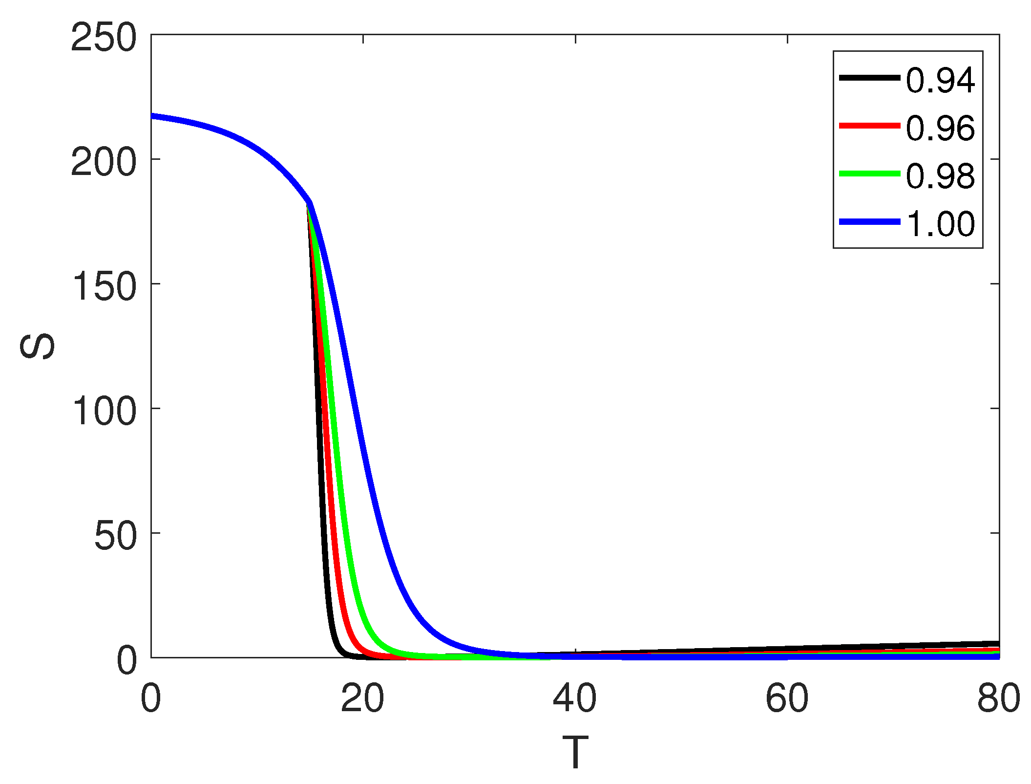
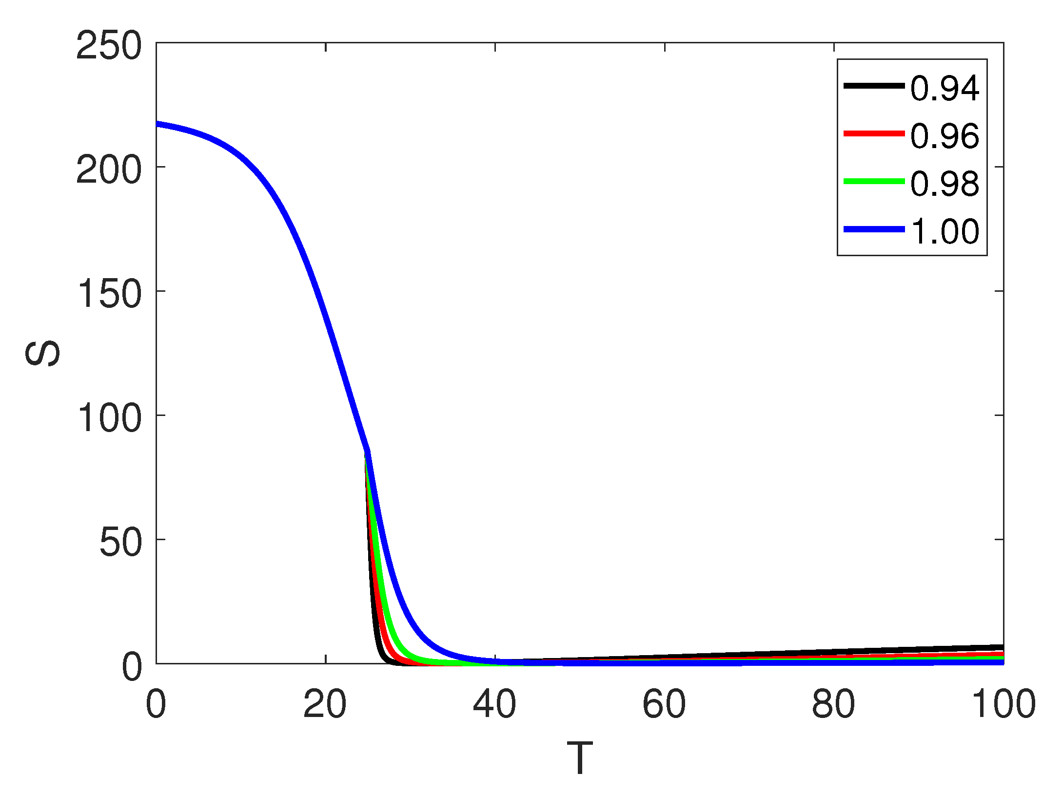
Figure 3 and Figure 4 represent, the susceptible population which declines and then becomes stable as the remaining classes increase on both intervals. The single curve is for the first interval and it shows integer order classical behavior from [ 0 , t 1 ] = [ 0 , 20 ] . While the four different curves show the global order derivative behavior on [ t 1 , t 2 ] = [ 20 , 80 ] . In Figure 4 the intervals are slightly increased and this also shows the same behavior.
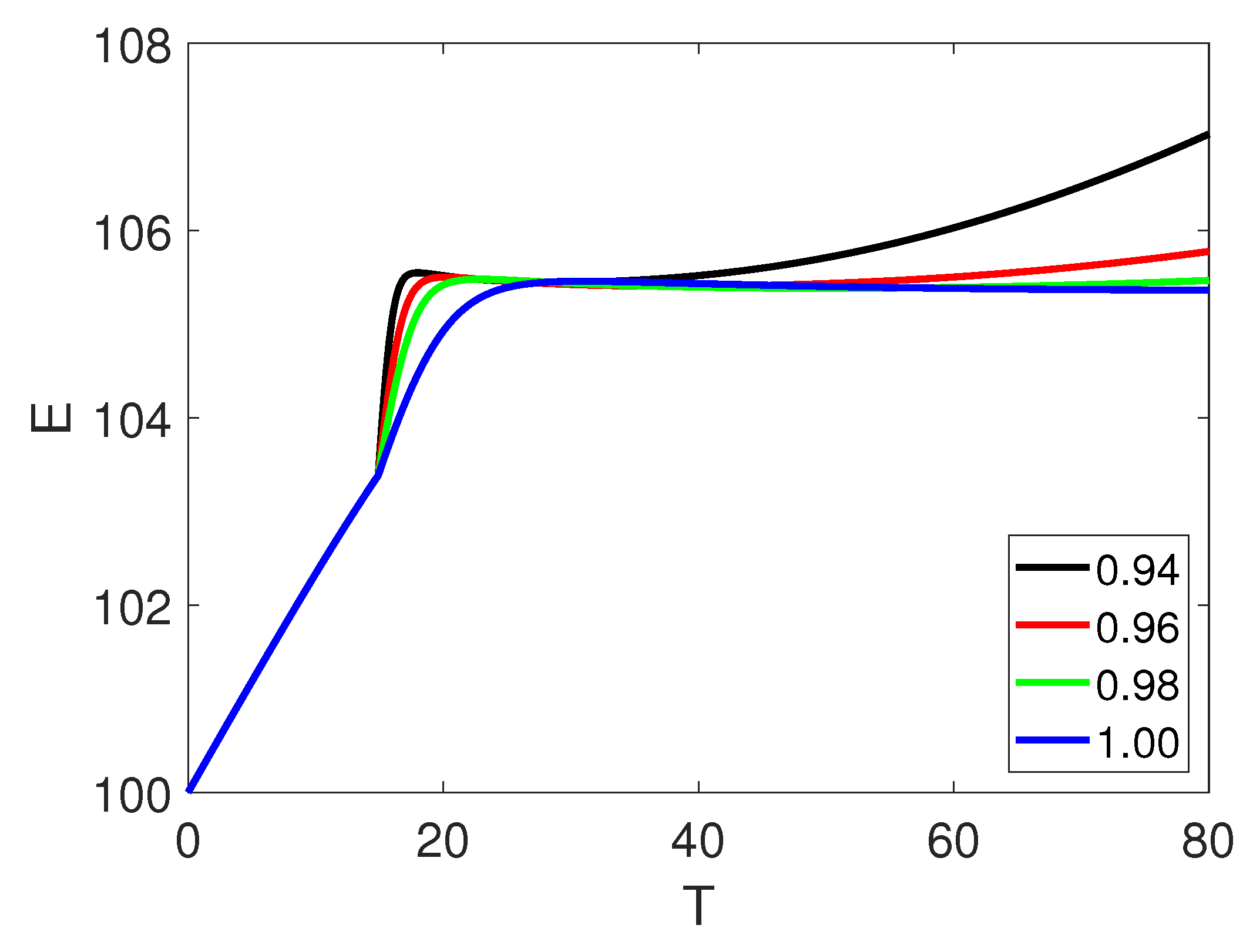
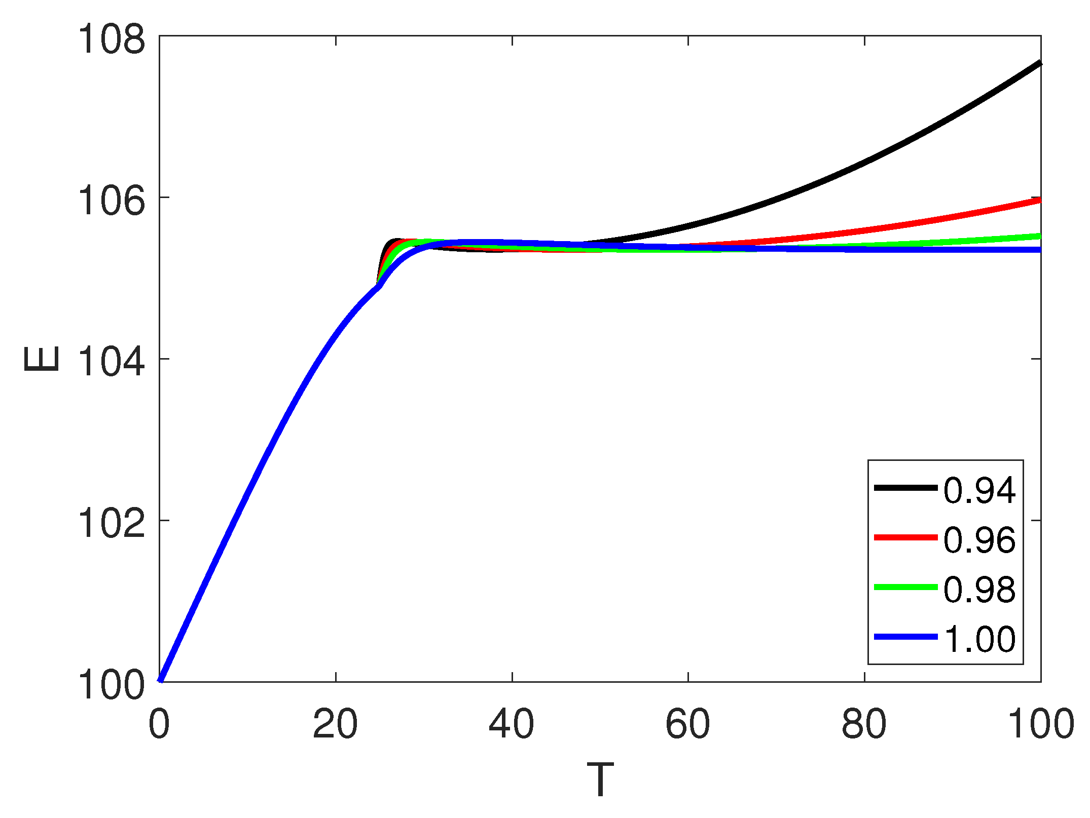
Next, Figure 5 and Figure 6 represent the exposed population which grows up and then becomes stable as the remaining two classes decline on both intervals. The single curve is for the first interval and it shows classical order dynamics on [ 0 , t 1 ] . While the four different curves show the fractional Caputo order derivative behavior on [ t 1 , t 2 ] . In Figure 6 the time interval is [0, 100], showing the same dynamics.
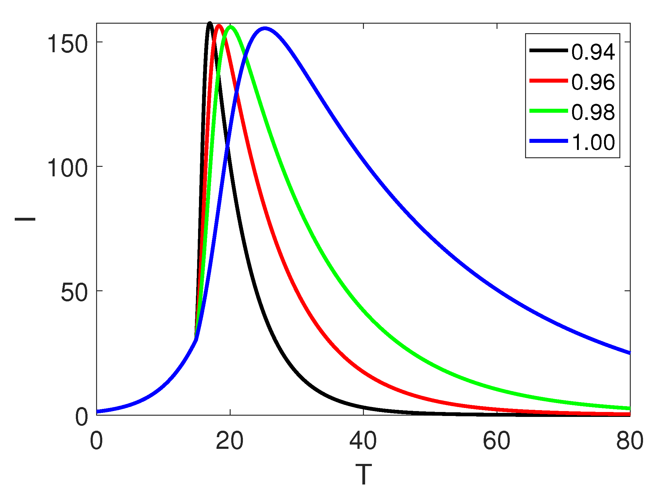
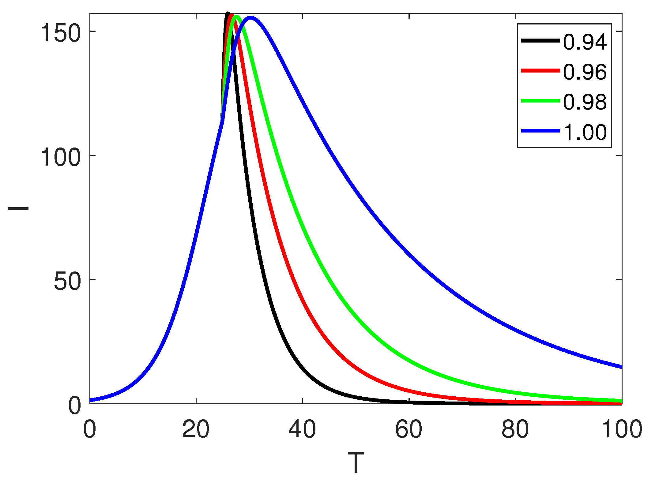
Furthermore, Figure 7 and Figure 8 show the infected population which grows up reaches up to its peak value, and then declines towards the convergent point. The first shows the integer order derivative, while the other show, the fractional Caputo derivative behavior on different fractional orders. In Figure 8 the time interval is changed, showing the same dynamics.
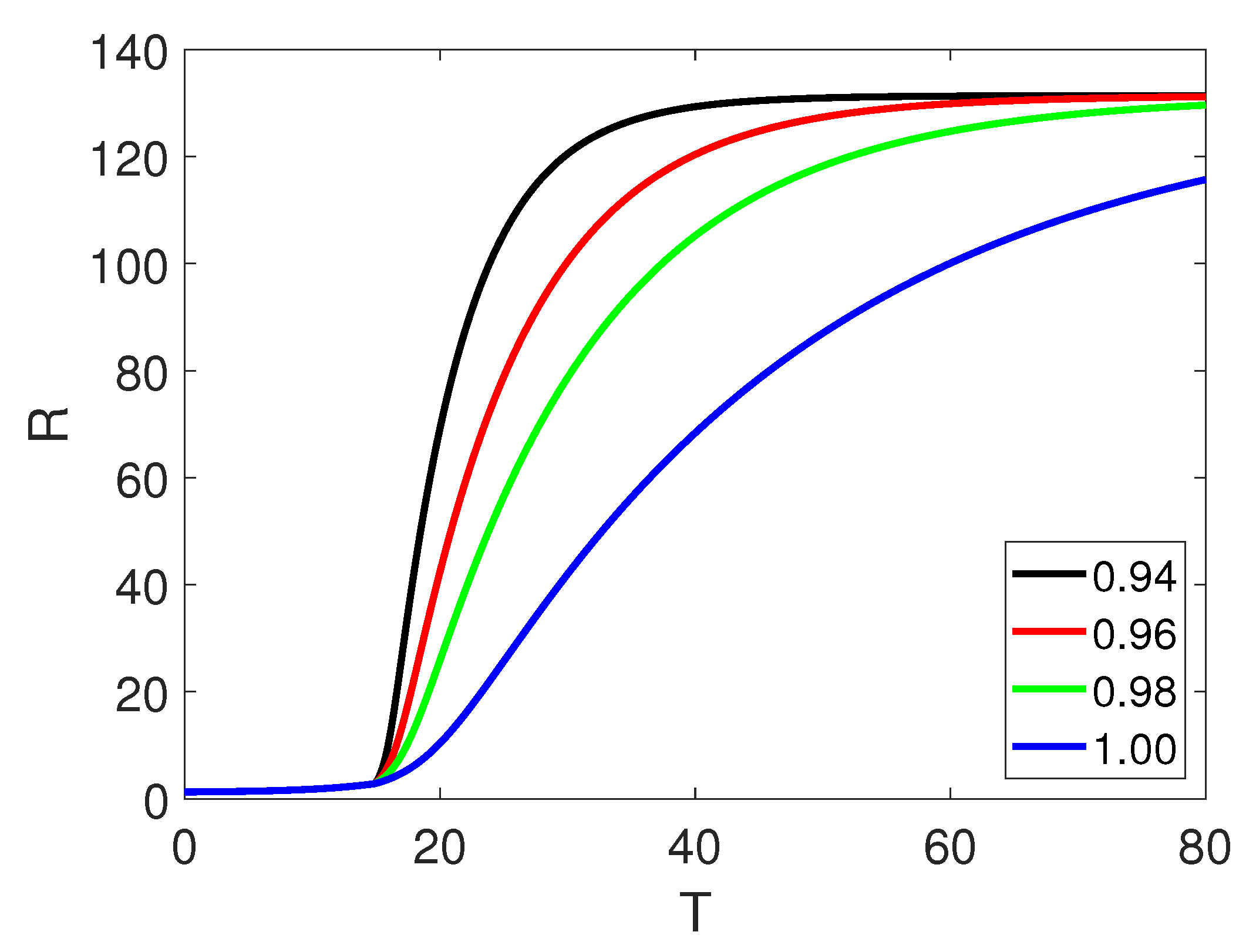
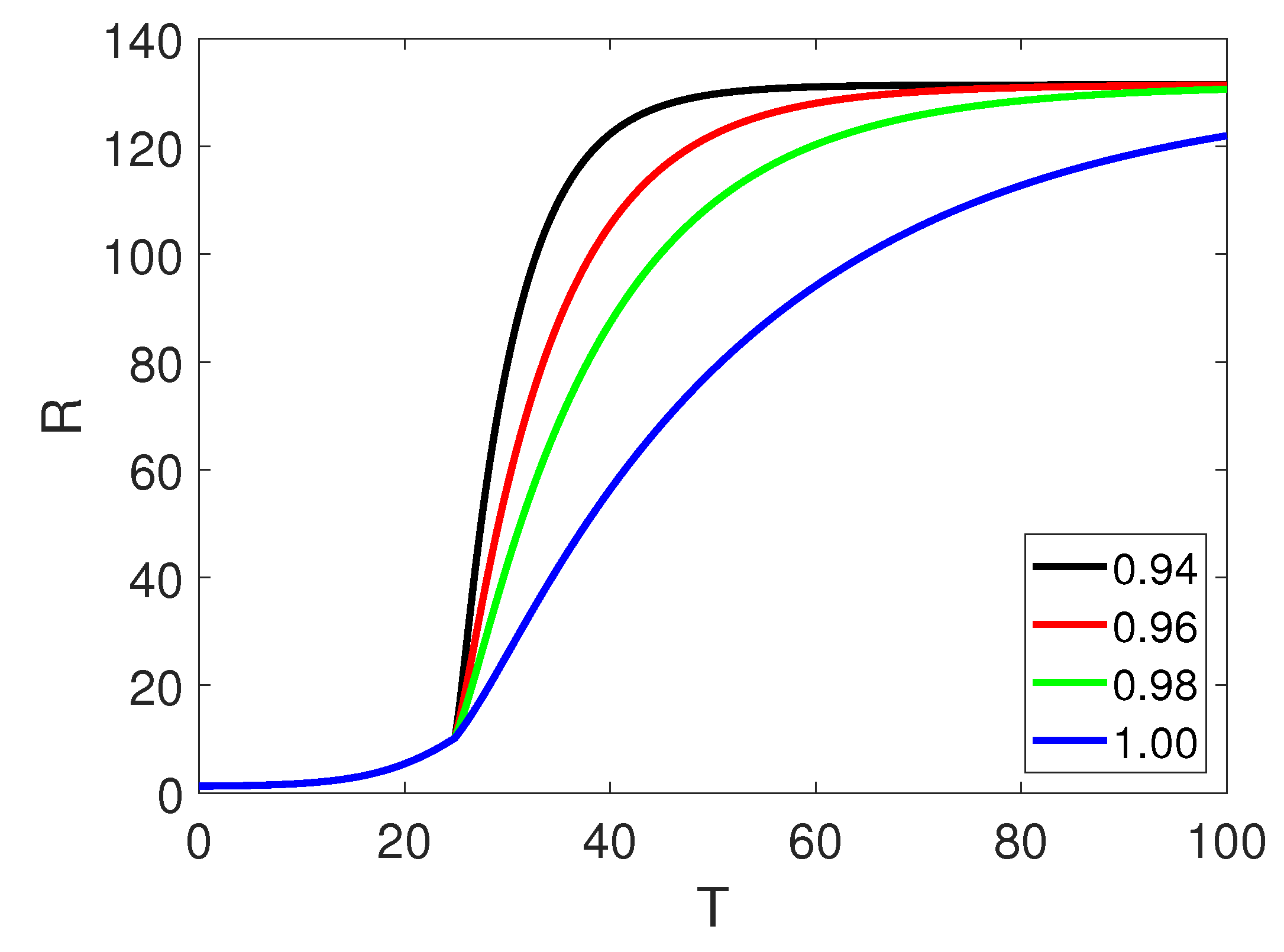
The dynamics of the recovered population are shown in Figure 9 and Figure 10, which indicate a sluggish increase at the first interval of integer order, followed by a fast increase that leads to the population’s stable value at the convergent point. The fractional Caputo order derivative dynamics are represented by the second interval, whilst the integer order derivative is represented by the first interval. The time interval is extended and the same dynamical behavior is displayed in Figure 10.
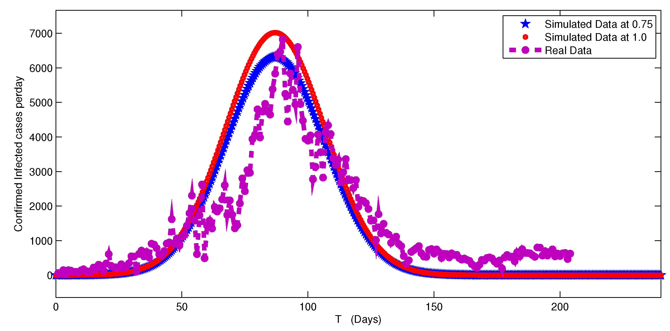
Here, we compare our results in ordinary form with some actual data for infected patients reported for 200 days in Pakistan using the citation style [56] at the specified fractional order. Similar to what is described in [60], the simulation is carried out. We can see that the simulated findings closely match those of actual data. This phenomenon shows that our plan and numerical analysis are valid. The relevant Figure is identified as Figure 11.

6. Discussion and Conclusion

In this paper, we developed a model based on the concept of piecewise equations with fractional order Caputo derivatives. We developed the existence theory of the proposed model’s solution using Schauder and Banach’s fixed point theory. In addition, a numerical scheme based on the Newton interpolation formula has been devised. The results were then graphically shown using real data for various fractional orders. Furthermore, in the case of stated infected persons, concerned results have been displayed and compared with real data. Because many real-world issues have abrupt shifts in their condition of rest or uniform motion, this is referred to as crossover behaviour. Traditional derivatives of either classical or fractional form cannot effectively depict this phenomenon. Using pieces-wise equations with fractional order derivatives, the aforementioned behaviour can be well explained. Furthermore, fractional order derivatives maintain a higher degree of freedom and flexibility. Figure 3, Figure 4, Figure 5, Figure 6, Figure 7, Figure 8, Figure 9 and Figure 10 show the crossover behavior at the indicated positions. Two sets of various fractional orders and time intervals have been used in the numerical simulation of all four compartments. The bending effects are also displayed when t 1 is used to describe the dynamics of piecewise derivatives.
The solutions and the integer order solution have also been compared. While the second interval is checked in multiple fractional orders, the first interval of the numerical simulation was given in integer order. Along with the comparison with integer order, both intervals are examined on fractional orders. Such an analysis can be used to examine numerous global occurrences when abrupt changes in the dynamics of several quantities occur. This enquiry can deal with the crossover aspects of both integer and fractional orders. In the end, we made a close comparison between our findings and some actual facts. Future applications of this style of analysis include more intricate dynamical issues including derivatives of the Mittag-Leffler and fractal-fractional types. The aforementioned model will then be examined utilizing singular and non-singular differential operators in the context of stochastic fractional order differential equations.

Data Availability Statement

All the data used in the paper is included in the manuscript.

Acknowledgments

The authors extend their appreciation to the Deputyship for Research Innovation, Ministry of Education in Saudi Arabia for funding this research through the project number IFP-IMSIU-2023126. The authors also appreciate the Deanship of Scientific Research at Imam Mohammad Ibn Saud Islamic University (IMSIU) for supporting and supervising this project.

Conflicts of Interest

The authors declare that they have no any kind of conflict of interest regarding this work.

References

  1. World Health Organization (WHO), Naming the coronavirus disease (COVID-19) and the virus that causes it,Archived from the original on 28 February 2020. Retrieved 28 February, 2020.
  2. D. S. I.Hui, et.al., The continuing 2019-nCoV epidemic threat of novel coronaviruses to global health-The latest 2019 novel coronavirus outbreak in Wuhan, China, Bulletin of Mathematical Biology, 91(6) (2020) 264-66. [CrossRef]
  3. S.Zhao, et. al, Preliminary estimation of the basic reproduction number of novel coronavirus (2019-nCoV) in China International Journal of Infectious Diseases 92 (2020) 214-217. [CrossRef]
  4. S.Zhao, et.al., Estimating the unreported number of novel coronavirus (2019-nCoV) cases in China in the first half of January 2020, a data-driven Modelling analysis of the early outbreak. J. Clin. Med., 9(2) (2020) 388. [CrossRef]
  5. I. Nesteruk, Statistics based predictions of coronavirus 2019-nCoV spreading in mainland China, MedRxiv, 4(1) (2020) 1988-1989. [CrossRef]
  6. K. Shah, R.U. Din, W. Deebani, P. Kumam, Z. Shah, On nonlinear classical and fractional order dynamical system addressing COVID-19, Results in Physics, 24 (2021) 104069. [CrossRef]
  7. J.A. Lotka, Contribution to the theory of periodic reactions, The Journal of Physical Chemistry, 14(3) (2002) 271-274. [CrossRef]
  8. N.S. Goel, S.C. Maitra, and E.W. Montroll, On the Volterra and other nonlinear models of interacting populations,Reviews of modern physics, 43(2) (1971) p.231. [CrossRef]
  9. M.M.Khalsaraei, An improvement on the positivity results for 2-stage explicit Runge-Kutta methods, J.Comput. Appl. Math., 235(1)(2010) 137-143. [CrossRef]
  10. P. Zhou, X.L. Yang, X.G. Wang, B. Hu, L. Zhang, W.Zhang, H.R.Si, Y. Zhu, B. Li, C.L. Huang, H.D.Chen, A pneumonia outbreak associated with a new coronavirus of probable bat origin. Nature, 579(7798) (2020) 270-273. [CrossRef]
  11. Q. Li, X. Guan, et.al., Early transmission dynamics in Wuhan, China, of novel coronavirus infected pneumonia, New England Journal of Medicine, 382 (2020) 1199-1207. [CrossRef]
  12. I.I. Bogoch, et.al., Pneumonia of unknown aetiology in Wuhan, China: potential for international spread via commercial air travel. Journal of travel medicine, 27(2) (2020) taaa008. [CrossRef]
  13. A.B. Gumel, et al., Modelling strategies for controlling SARS out breaks, Proc. R. Soc. Lond. B, 271(1554) (2004) 2223–2232. [CrossRef]
  14. R. Kahn, I. Holmdahl, S. Reddy, J. Jernigan, M.J. Mina, R.B.Slayton, Mathematical Modeling to Inform Vaccination Strategies and Testing Approaches for Coronavirus Disease 2019 (COVID-19) in Nursing Homes, Clinical Infectious Diseases, 74(4) (2022) 597-603. [CrossRef]
  15. J. Mondal and S. Khajanchi, Mathematical modeling and optimal intervention strategies of the COVID-19 outbreak, Nonlinear Dynamics, 2022 (2022), 1-26. [CrossRef]
  16. S. Hussain, et.al., On the Stochastic Modeling of COVID-19 under the Environmental White Noise, Journal of Function Spaces, 2022 (2022), Article ID 4320865, 9 pages. [CrossRef]
  17. J.T. Wu, K. Leung, G.M. Leung, Nowcasting and forecasting the potential domestic and international spread of the 2019-nCoV outbreak originating in Wuhan, China: a modelling study, The Lancet, 395(10225) (2020) 689-697. [CrossRef]
  18. J.T.Machado, V. Kiryakova, F. Mainardi, Recent history of fractional calculus, Commun. Nonl. Sci. Numer. Simul., 16(3) (2011) 1140-1153. [CrossRef]
  19. F.C. Meral, T.J. Royston, R. Magin, Fractional calculus in viscoelasticity: an experimental study. Commun. Nonl. Sci. Numer. Simul., 15(4) (2010) 939-945. [CrossRef]
  20. L.M. Richard, Fractional calculus in bioengineering, part 1, Critical Reviews in Biomedical Engineering 32(1) (2004). [CrossRef]
  21. M. Dalir, M. Bashour, Applications of fractional calculus, Appl. Math. Sci., 4(21) (2010) 1021-1032. [CrossRef]
  22. L.M. Richard, Fractional Calculus in Bioengineering. Vol. 2. No. 6. Redding: Begell House, 2006. [CrossRef]
  23. A.Y.Rossikhin and M. V. Shitikova, Applications of fractional calculus to dynamic problems of linear and nonlinear hereditary mechanics of solids, (1997), 15-67. [CrossRef]
  24. F. Mainardi, Fractional calculus. In Fractals and fractional calculus in continuum mechanics, Springer, Vienna, 1997.
  25. M.M.Matar, M. I. Abbas, J. Alzabut, M.K.A. Kaabar, S. Etemad, S. Rezapour, Investigation of the p-Laplacian nonperiodic nonlinear boundary value problem via generalized Caputo fractional derivatives. Advances in Difference Equations, 2021(1) (2021) 1-18. [CrossRef]
  26. M.Shimizu and W. Zhang, Fractional calculus approach to dynamic problems of viscoelastic materials. JSME Int. J.Ser. C. Mech. Sys. Mach. Ele. Manuf., 42(4) (1999) 825-837. [CrossRef]
  27. F. Mainardi, An historical perspective on fractional calculus in linear viscoelasticity, Fractional Calculus and Applied Analysis,15(4) (2012) 712-717. [CrossRef]
  28. Z. Dai, et al., A model of lung parenchyma stress relaxation using fractional viscoelasticity, Medical Eng. Physics, 37(8) (2015) 752-758. [CrossRef]
  29. M. M. Amirian and Y.Jamali, The concepts and applications of fractional order differential calculus in modeling of viscoelastic systems: a primer, Critical Reviews in Biomedical Engineering 47( 4) (2019) 1-35. [CrossRef]
  30. H. Khan, J.F. Gómez-Aguilar, A. Alkhazzan, A. Khan, A fractional order HIV-TB coinfection model with nonsingular Mittag-Leffler Law, Mathematical Methods in the Applied Sciences, 43(6)(2020) 3786-3806. [CrossRef]
  31. C. Celauro, C. Fecarotti, A. Pirrotta, and A. C. Collop, Experimental validation of a fractional model for creep/recovery testing of asphalt mixtures, Construction and Building Materials, 36( 2012) 458-466. [CrossRef]
  32. G.C.Wu, M. Luo, L.L. Huang, S. Banerjee, Short memory fractional differential equations for new memristor and neural network design, Nonlinear Dynamics, 100(4) (2020) 3611-3623. [CrossRef]
  33. A. Atangana, D. Baleanu, New fractional derivatives with non-local and non-singular kernel. Theory Appl Heat Transf Model Therm Sci 20(2) (2016) 763-9. [CrossRef]
  34. E.F.D. Goufo, Application of the Caputo-Fabrizio fractional derivative without singular kernel to Korteweg-de Vries-Burgers equation, Math Model Anal, 21(2)(2016) 188-98. [CrossRef]
  35. E.F.D. Goufo, A bio mathematical view on the fractional dynamics of cellulose degradation, Fract. Calc. Appl. Anal., 18(3)(2015) 554-64. [CrossRef]
  36. R.Begum, O. Tunç, H. Khan, H. Gulzar, A. Khan, A fractional order Zika virus model with Mittag-Leffler kernel, Chaos, Solitons & Fractals, 146 (2021) 110898. [CrossRef]
  37. A. Atangana, S.I.Araz, Nonlinear equations with global differential and integral operators:existence, uniqueness with application to epidemiology, Results in Phy., 20 (2021): 103593. [CrossRef]
  38. S.K. Kabunga, E.F.D.Goufo, V. H. Tuong. Analysis and simulation of a mathematical model of tuberculosis transmission in democratic Republic of the Congo, Adv. Differ. Equ., (1)(2020) 1-19. [CrossRef]
  39. A. Atangana, S.I. Araz, Mathematical model of COVID-19 spread in Turkey and South Africa: theory, methods and applications, Adv Differ Equ 2020 (2020):659. [CrossRef]
  40. A. Atangana, S. I. Araz, New concept in calculus:Piecewise differential and integral operators, Chaos Soliton. Fract., 145 (2021) 110638. [CrossRef]
  41. M.A. Khan and A. Atangana, Modeling the dynamics of novel coronavirus (2019-nCov) with fractional derivative, Alexandria Engineering Journal, 59(4) (2020) 2379-2389. [CrossRef]
  42. M.A. Khan, A. Atangana, E. Alzahrani, The dynamics of COVID-19 with quarantined and isolation, Advances in Difference Equations, 2020(1) (2020) 1-22. [CrossRef]
  43. S. Boccaletti, W. Ditto, G. Mindlin, A. Atangana, Modeling and forecasting of epidemic spreading: The case of Covid-19 and beyond, Chaos, Solitons, and Fractals, 135 (2020) 109794. [CrossRef]
  44. E. Atangana, A.Atangana, Facemasks simple but powerful weapons to protect against COVID-19 spread: Can they have sides effects?. Results in Physics, 19 (2020) 103425. [CrossRef]
  45. A.Zeb, A. Atangana, Z.A. Khan and S. Djillali, A robust study of a piecewise fractional order COVID-19 mathematical model. Alexandria Engineering Journal, 61(7) (2022), pp.5649-5665. [CrossRef]
  46. S. Boccaletti, D. William, G. Mindlin, and A. Atangana, Modeling and forecasting of epidemic spreading: The case of Covid-19 and beyond, Chaos, Solitons and Fractals, 135 (2020) 109794. [CrossRef]
  47. M.S.Arshad.et.al, A Novel 2-Stage Fractional Runge-Kutta Method for a Time Fractional Logistic Growth Model, Discrete Dynamics in Nature and Society, 2020 (2020), Article ID 1020472, 8 pages. [CrossRef]
  48. F. Liu, K. Burrage, Novel techniques in parameter estimation for fractional dynamical models arising from biological systems, Comput. Math. Appl., 62(3) (2011) 822-833. [CrossRef]
  49. M.T.Hoang, O.F. Egbelowo, Dynamics of a fractional-order hepatitis B epidemic model and its solutions by nonstandard numerical schemes, Mathematical Modelling and Analysis of Infectious Diseases, 2020 (2020) 127-153. [CrossRef]
  50. F. Zhuo-Jia, et al. Numerical solutions of the coupled unsteady nonlinear convection-diffusion equations based on generalized finite difference method, The European Physical Journal Plus 134(6) (2019) 1-20. [CrossRef]
  51. B. Wang, L. Li, Y. Wang, An efficient nonstandard finite difference scheme for chaotic fractional-order Chen system. IEEE Access, 8 (2020) 98410-98421. [CrossRef]
  52. A.J.Arenas, G. González-Parra, B.M. Chen-Charpentier, Construction of nonstandard finite difference schemes for the SI and SIR epidemic models of fractional order, Math. Comput. Simul., 121 (2016) 48-63. [CrossRef]
  53. R. Lewandowski, and Z. Pawlak, Dynamic analysis of frames with viscoelastic dampers modelled by rheological models with fractional derivatives, Journal of sound and Vibration, 330(5) (2011) 923-936. [CrossRef]
  54. https://www.worldometers.info/world-population/pakistan-population/ 25 January 2022.
  55. https://www.coronatracker.com/country/pakistan/ 10 December 2021.
  56. www.worldometers.info, Current information about COVID-19 in Pakistan, 18 January, 2021.
  57. A Al Elaiw, F Hafeez, MB Jeelani, M Awadalla, K Abuasbeh .Existence and uniqueness results for mixed derivative involving fractional operatorsAIMS Mathematics 8 (3), 7377-7393.
  58. Jeelani, M. B. (2023). STABILITY AND COMPUTATIONAL ANALYSIS OF COVID-19 USING A HIGHER ORDER GALERKIN TIME DISCRETIZATION SCHEME. Advances and Applications in Statistics, 86(2), 167–206. https://doi.org/10.17654/0972361723022. [CrossRef]
  59. A Moumen, R Shafqat, A Alsinai, H Boulares, M Cancan, MB Jeelani ,Analysis of fractional stochastic evolution equations by using Hilfer derivative of finite approximate controllability. AIMS Math 8, 16094-16114. [CrossRef]
  60. K. Shah, T. Abdeljawad, R. Din, To study the transmission dynamic of SARS-CoV-2 using nonlinear saturated incidence rate, Physica A: Statistical Mechanics and its Applications, 604 (2022) 127915. [CrossRef]
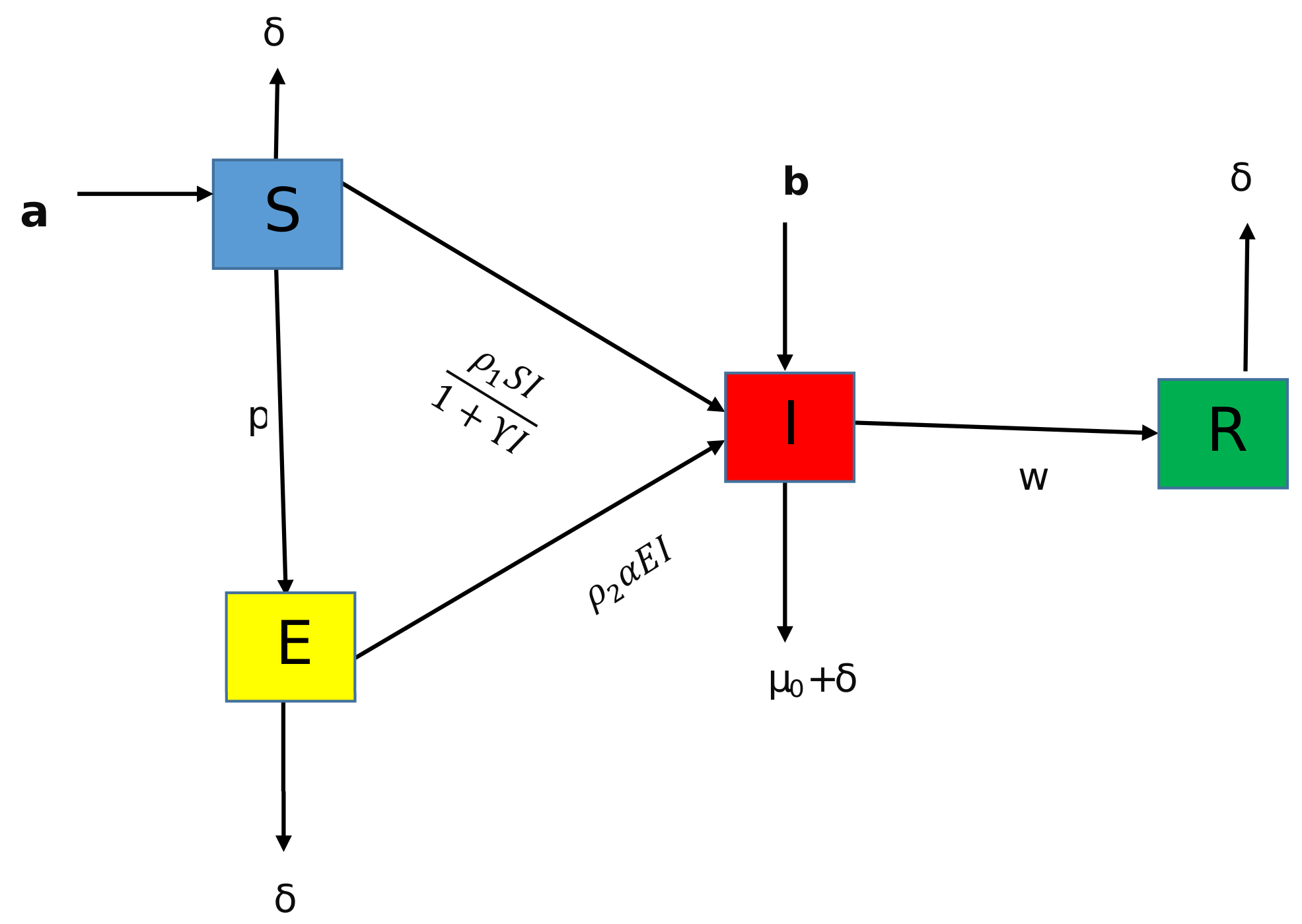
Figure 1. Flow Chart of our established Model (1).
Preprints 77600 g001
Figure 2. 3D profile of R 0 computed in (5).
Preprints 77600 g002
Figure 3. Piecewise representation of approximate solution for S for classical derivative on [ 0 , t 1 ] and fractional order derivative on [ t 1 , t 2 ] of order r .
Preprints 77600 g003
Figure 4. Piecewise representation of approximate solution for S for classical derivative on [ 0 , t 1 ] and fractional order derivative on [ t 1 , t 2 ] of order r .
Preprints 77600 g004
Figure 5. Piecewise representation of approximate solution for E for classical derivative on [ 0 , t 1 ] and fractional order derivative on [ t 1 , t 2 ] of order r .
Preprints 77600 g005
Figure 6. Piecewise representation of approximate solution for E for classical derivative on [ 0 , t 1 ] and fractional order derivative on [ t 1 , t 2 ] of order r .
Preprints 77600 g006
Figure 7. Piecewise representation of approximate solution for I for classical derivative on [ 0 , t 1 ] and fractional order derivative on [ t 1 , t 2 ] of order r .
Preprints 77600 g007
Figure 8. Piecewise representation of approximate solution for I for classical derivative on [ 0 , t 1 ] and fractional order derivative on [ t 1 , t 2 ] of order r .
Preprints 77600 g008
Figure 9. Piecewise representation of approximate solution for R for classical derivative on [ 0 , t 1 ] and fractional order derivative on [ t 1 , t 2 ] of order r .
Preprints 77600 g009
Figure 10. Piecewise representation of approximate solution for R for classical derivative on [ 0 , t 1 ] and fractional order derivative on [ t 1 , t 2 ] of order r .
Preprints 77600 g010
Figure 11. Comparison of per day infected cases with that of simulated data of our proposed model.
Preprints 77600 g011
Table 1. Parameters and their discerption of the model (1).
Nomenclature Representation
S Susceptible class
E Exposed class
I Infected class
R Recovered class
N 0 Total initial papulation
N Total population at time t
b Immigrant to I from E
μ 0 infection death rate
δ death rate due to natural way
a Recruitment rate
p Migration rate from S to E
γ Saturation value of virus
α rate at which infection is reducing
ρ 1 contact rate
w rate at which individual gets ride from infection
ρ 2 infection rate
Table 2. Numerical values of the nomenclatures of the model.
Nomenclature Numerical value
S 217.342565 in millions[54]
E 100 in million (assumed)
I 1.386348 in million[54]
R 1.271087 in million [54]
b 0.135 (assumed) d a y 1
μ 0 0.19 [54] d a y 1
δ 0.000065 [54] d a y 1
a 1.43 (assumed) d a y 1
p 0.45 d a y 1
γ 0.00019 (assumed) d a y 1
α 0.0008601 (assumed) d a y 1
ρ 1 0.10 (assumed) d a y 1
w 0.98 (assumed) d a y 1
ρ 2 0.020 (assumed) d a y 1
Disclaimer/Publisher’s Note: The statements, opinions and data contained in all publications are solely those of the individual author(s) and contributor(s) and not of MDPI and/or the editor(s). MDPI and/or the editor(s) disclaim responsibility for any injury to people or property resulting from any ideas, methods, instructions or products referred to in the content.
Copyright: This open access article is published under a Creative Commons CC BY 4.0 license, which permit the free download, distribution, and reuse, provided that the author and preprint are cited in any reuse.
Prerpints.org logo

Preprints.org is a free preprint server supported by MDPI in Basel, Switzerland.

Subscribe

© 2024 MDPI (Basel, Switzerland) unless otherwise stated