1. Introduction
There has been a significantly increase in the use of deep learning (DL) models to conduct multivariate time series (TS) data analysis in many key application areas; such as banking, healthcare, environment, and other areas that benefit society; as well as crucial infrastructures that are powered by the Internet of Things or the climate.
Quantitative system dynamics data from historical performance and qualitative fundamental data from various news sources affect the performance of TS data obtained from economic markets. As both these types of data can be combined to effectively identify patterns in economic data, it is currently of significant interest and researched by both professionals and academics alike. Most extant studies have used data that has been derived from news sources to estimate the direction of stock movements. However, this caused a classification problem, which was the exact price of an asset in the future, which poses a regression problem. Therefore, this present study hypothesised that using multiple datasets obtained from the Saudi Stock Exchange (Tadawul); specifically opening, lowest, highest, and closing prices; to conduct a multivariate analysis increases the accuracy of the forecasted future price of a stock.
As stock market predictions heavily rely on a combination of mental vs. physical characteristics and rational vs. illogical behaviours to yield stable values, they are extremely difficult to precisely anticipate. As such, it is one of the most significant topics in the computer science industry at present.
Stock market prices for the next 10 days can be predicted by analysing a financial timeline over an extended period of time. Extant studies indicate that significantly accurate stock price forecasts can be made using accurate coding. Nevertheless, some studies suggest that market hypotheses and predictions are merely hypothetical and inaccurate.
Multiple models have been proposed to forecast stock prices. The variables chosen, the analysis method, and the modelling process significantly affect the forecasting accuracy of a model. Deep learning (DL) and machine learning (ML) have been frequently used to analyse and predict stock prices. Artificial intelligence (AI), a field of study in computer science and technology, has made considerable strides in recent years and significantly simplified multiple real-world problems.
As there are multiple variables that affect a prediction, it is simpler to project the weather or a certain trait than the stock market as it is a constant state of flux. More specifically, stock prices fluctuate independently at the times since financial markets have regular ups and downs. Therefore, compiling accurate historical data is no small feat as the stock market is volatile. Moreover, a variety of factors; such as economic, business, personal, political, and social issues; could affect the market. As such, it is virtually impossible to predict changes in stock prices due to the stock market's extreme unpredictability. Globalisation as well as the development of information and communication technology (ICT) has increased the number of individuals seeking to make exorbitant returns from the stock market. As such, stock market predictions have become crucial for investors.
The fundamental method and the technical method are the two different methods of forecasting the stock market. Unlike the technical method, which uses analyses graphs to forecast future stock prices, the fundamental method examines every facet of a firm's internal worth. However, the fundamental method is not without drawbacks as it generates fewer time predictions and lacks compliance. As such, many stock market prediction studies utilise the technical method. Moving averages, genetic algorithms, easy measurement, regression, and support vector machines (SVMs) are some of the ML methods that have been employed to address this issue. However, none of them produce predictions that are extremely precise. This has given rise to the use of mixed method approaches. Although problem-solving methods have been around for a while, in the data science industry, these are some of the most difficult issues to solve as many significant concerns are involved when predicting future prices and spotting trends in stock market data.
This present study examined a method that uses a long short-term memory (LSTM) or temporary memory algorithm. A potent technique for handling TS data is the recurrent neural network (RNN). In many ways, LSTMs are subordinate to sensory RNN networks and feed broadcasts (Alabdulkreem et al., 2023). This is due to the fact that, by choosing long patterns, they possess a commemorative quality. Few RNN models have been utilised to predict movements in the stock market. A LSTM is one of the most effective RNN structures. This present study discusses the distinctions between univariate and multivariate analysis as it primarily examines multivariate TS analysis. A TS that only contains one variable is referred to as a univariate TS. A TS data's value at time step 't' is basically derived from its preceding time steps; t-1, t-2, t-3, and so on. Unlike multivariate models, univariate models are easier to construct. The closing price of a capital asset is typically the variable of interest when predicting stock prices (D. Kim & Baek, 2022).
Unlike a univariate TS, multivariate TSs do not contain single dependent variables but several interconnected variables (Dinh, Thirunavukkarasu, Seyedmahmoudian, Mekhilef, & Stojcevski, 2023). It also considers numerous influencing aspects as well as non-influencing aspects. Predicting stock market prices using multivariate analysis depends on many different variables; such as opening, highest, lowest, and closing prices. Therefore, multivariate models are typically more challenging (Tai, Wang, & Huang, 2023) to develop than univariate models. This poses difficulties including the management of several parameters in a high dimensional space (Tuli, Casale, & Jennings, 2022).
This present study concentrates on the short-term price behaviour of the communication industry, which is made up of three major firms: Etihad Etisalat (Mobily), Saudi Telecom Company (STC), and Zain KSA. These three businesses were chosen as best they reflect the economy of the Kingdom of Saudi Arabia (KSA) in the Saudi Stock Exchange (Tadawul) as they are heavily traded. The KSA's communication industry is among the largest and fastest emerging markets in North Africa and the Middle East, with Mobily, STC, and Zain KSA as the top players in the mobile market. In 2022, the combined market valuation of these three firms surpassed 58 billion Saudi riyals.
This present study:
Outlines what is required to conduct a TS analysis as well as demonstrates how each of the univariate and multivariate models examined are satisfied and applied to the proposed LSTM DL.
Provides an in-depth theoretically-based comparison of the resilience, memory consumption, stability, flow control, and robustness of univariate and multivariate TSs as well as thoroughly examines the mathematical logic and internal structure of both TSs to explain why a multivariate TS is better than a univariate TS.
Uses real datasets to depict the results of the experimental analysis, which indicated that other prices affect the predictive accuracy of the proposed LSTM DL.
Chapter 1 provides an introduction to the researched topic while Chapter 2 discusses relevant extant studies and how the present study differs from them. In Chapter 3, the dataset that this present study used is discussed. Chapter 4 outlines the methodology that was used to develop the proposed LSTM DL while Chapter 5 discusses the prediction algorithm of the proposed LSTM DL. Chapter 6 outlines forecasting methods and Chapter 7 provides the results of the experiment. The accuracy of the the proposed LSTM DL is examined in Chapter 8 while, in Chapter 9, existing models are fitted with the proposed LSTM DL and the conclusion is discussed.
2. Literary Survey
It is essential to review extant studies prior to conducting a research. The experimental findings of Liu and Long (2020) demonstrated that the proposed hybrid framework, which could be used for fiscal data analysis and research or stock market monitoring, had the best projection accuracy. As the primary component of the mixed framework, a dropout strategy and particle swarm optimisation (PSO) were used to augment a DL network predictor that was based on a LSTM network. The proposed framework for projecting stock closing prices outperformed conventional models in terms of prediction. Theoretically, the LSTM network is particularly well suited for financial TS projection due of its cyclic nature, which gives it the function of long-term memory. The deep hybrid framework's components included data processing, a DL predictor, and the predictor optimisation technique (Liu & Long, 2020).
Nabipour et al. (2020) used bagging, decision tree, random forest, gradient boosting, adaptive boosting (AdaBoost), eXtreme gradient boosting (XGBoost), RNN, artificial neural networks (ANN), and LSTM. Different ML techniques were used to forecast future stock market group values. From the Tehran Stock Exchange, four groups; i.e., petroleum, diversified financials, non-metallic minerals, and basic metals; were selected for experimental assessments. Due to its intrinsic subtleties, non-linearity, and complexity, the estimation of stock group prices has long been appealing to and challenging for investors (Nabipour, Nayyeri, Jabani, Mosavi, & Salwana, 2020).
Manujakshi et al. (2022) used a hybrid prediction rule ensembles (PRE) and deep neural networks (DNN) stock prediction model to address nonlinearity in the examined data. The mean absolute error (MAE) and root-mean-square-error (RMSE) metrics were used to calculate the results of the hybrid PRE-DNN stock estimation model. The stock prediction rules with the lowest RMSE score was selected from all the stock prediction rules generated using the PRE approach. As it improved the RMSE by 5% to 7%, the hybrid PRE-DNN stock estimation model outperformed DNN and ANN single prediction models. Because of the many aspects which affect the stock market, including corporate earnings, geopolitical tension, and commodity prices, stock prices are prone to volatility (Manujakshi, Kabadi, & Naik, 2022).
The single-layer RNN model suggested by Zaheer et al. (2023) improved prediction accuracy by 2.2%, 0.4%, 0.3%, 0.2%, and 0.1%. The experimental findings supported the efficacy of the proposed prediction methodology, which helps investors increase their earnings by selecting wisely. The model uses the input stock data to anticipate the closing price and highest price of a stock for the following day. The obtained results demonstrated that CNN performed the worst while the LSTM outperformed the CNN-LSTM, the CNN-RNN outperformed the CNN-LSTM and the LSTM, and the proposed single-layer RNN model outperformed all of them. Due to the non-linearity, substantial noise, and volatility of TS data on stock prices, stock price estimation is highly difficult (Zaheer et al., 2023).
Kim et al. (2022) proposed methods of predicting the oil prices of Brent Crude and West Texas Intermediate (WTI) using multivariate TS of key S&P 500 stock prices, Gaussian process modelling, vine copula regression, DL, and a smaller number of significant covariates. The 74 large-cap key S&P 500 stock prices and the monthly log returns of the oil prices of both companies for the timespan of February 2001 to October 2019 were used to test the proposed methods on actual data. With regards to the extent of prediction errors, the vine copula regression with NLPCA was generally superior to other proposed approaches. To reduce the dimensions of the data, a Bayesian variable selection and nonlinear principal component analysis (NLPCA) were used (J.-M. Kim, Han, & Kim, 2022).
Munkhdalai et al. (2022) used a unique locally adaptable and interpretable DL architecture supplemented with RNNs to render model explainability and superior predictive accuracy for time-series data. The experimental findings using publicly available benchmark datasets demonstrated that the model not only outperformed state-of-the-art baselines in terms of prediction accuracy but also identified the dynamic link between input and output variables. Next, to make the regression coefficients adjustable for each time step, RNNs were used to re-parameterise the basic model. A simple linear regression and statistical test were used to establish the base model. In time-dependent fields like finance and economics that depend on variables, explaining dynamic relationships between input and output variables is one of the most crucial challenges (Munkhdalai et al., 2022).
According to Charan et al. (2022), the Prophet model based on logistic regression had the lowest RMSE value of all the other algorithms, therefore, it was the most effective. A firm's growth and advancement can be easily predicted by examining its stock market performance, which paves the way for the advancement of stock price projection technology to determine the effects of any event occurring in the modern world. Four supervised ML models; Facebook Prophet, multivariate linear regression, autoregressive integrated moving average (ARIMA), and LSTM; were used to predict the closing stock price of Tata Motors, a major Indian automaker, while RMSE was used to determine efficacy (Charan, Rasool, & Dubey, 2022).
The introduction of an automated system which can predict potential stock prices with significant precision is important as it is not humanly possible for stock market traders and investors to comprehend the nature of fluctuations in prices. Forecasting future stock market trends is unfortunately quite difficult due to the unpredictable, non-linear, and volatile character of stock market values. Uddin et al. (2022) demonstrated the promising potential of their proposed architecture by examining data from the Dhaka Stock Exchange. In order to reduce investment risks, it is crucial for the interested parties and stakeholders to possess suitable and insightful trends of stock prices (Uddin, Alam, Das, & Sharmin, 2022)
Domala and Kim (2022) predicted the significant wave height using ML and DL techniques. Regression models, SVMs, and DL models; such as LSTM and CNN; were used to conduct univariate and multivariate analyses. The suggested models were a superb technique for forecasting the significant wave height. The inputs used to estimate significant wave heights included wind direction, wind speed, wind pressure, gust speed, and sea surface temperature. The basis of these inputs was correlations with the target feature. In order to analyse the data type, exploratory data analysis was conducted on the gathered meteorological wave data. The data was then filtered and put into the ML algorithms (Domala & Kim, 2022).
Stock values can be easily predicted using ML algorithms on data from financial news, which can also impact investors' interests. Precise prediction analysis is essential for evaluating stock values and their ups and downs throughout time because stock markets are, by their very nature, unpredictable. According to Thangamayan et al. (2022), DL technology has made it possible to anticipate stock prices with precision. The study predicted the stock market using numerous models. On the other hand, using conventional prediction methods with non-stationary TS data is no longer successful (Thangamayan et al., 2022).
Youness and Driss (2022) examined and compared the LSTMDL and ARIMA algorithms for a univariate TS, particularly for stock prices. Classical approaches; such as ARIMA; outperformed DLs as they are very straightforward to use, particularly for linear univariate datasets. The performance was measure using MAE, mean absolute percentage error (MAPE), or root-mean-square deviation and the extracted dataset. The LSTMDL algorithms were more potent and produced superior projections (Youness & Driss, 2022).
Using an RNN and discrete wavelet transform (DWT), Jarrah and Salim (2019) sought to forecast Saudi stock price trends based on its historic prices. A comparison indicated that the proposed DWT-RNN method provided for a more precise estimation of the day's closing price using MAE, mean squared error (MSE), and RMSE than the ARIMA method. The developed RNN was trained using the back propagation through time (BPTT) approach to assist in forecasting the closing price of the Saudi market's stocks for the selected sample of firms for the upcoming seven days. The noise around the data collected from the Saudi stock market was reduced with the help of the DWT technique. The results were then analysed and compared to that of more conventional prediction algorithms; such as ARIMA (Jarrah & Salim, 2019).
3. Research Dataset
This present study used Tadawul All Share Index-Saudi Arabia (TASI) stocks from Infosys and Reliance with historical prices spanning a total of 1472 days, from 1 January 2017 to 21 November 2022. All the data required for this present study was gathered from investing.com (
https://www.investing.com/indices/ttisi).
Table 1,
Table 2 and
Table 3 provide excerpts of each company.
Table 1.
A snippet of STC stock prices.
Table 1.
A snippet of STC stock prices.
| Date |
Closing |
Opening |
Highest |
Lowest |
| 21/11/2022 |
37.75 |
37.8 |
37.85 |
37.65 |
| 20/11/2022 |
37.8 |
37.85 |
37.85 |
37.6 |
| 17/11/2022 |
37.65 |
38 |
38.05 |
37.65 |
| 16/11/2022 |
38 |
37.8 |
38 |
37.15 |
| 15/11/2022 |
37.8 |
38.3 |
38.3 |
37.5 |
| 14/11/2022 |
38.3 |
38.25 |
38.5 |
38 |
Table 2.
A snippet of Mobily stock prices.
Table 2.
A snippet of Mobily stock prices.
| Date |
Closing |
Opening |
Highest |
Lowest |
| 21/11/2022 |
35.45 |
35.2 |
35.65 |
34.9 |
| 20/11/2022 |
35.85 |
36.5 |
36.5 |
35.2 |
| 17/11/2022 |
36.45 |
35.85 |
36.5 |
35.55 |
| 16/11/2022 |
36.1 |
35 |
36.5 |
35 |
| 15/11/2022 |
35 |
35.8 |
36 |
34.95 |
| 14/11/2022 |
36 |
36.3 |
36.8 |
35.8 |
Table 3.
A snippet of Zain KSA stock prices.
Table 3.
A snippet of Zain KSA stock prices.
| Date |
Closing |
Opening |
Highest |
Lowest |
| 24/11/2022 |
11.06 |
11.32 |
11.32 |
11.06 |
| 22/11/2022 |
11.4 |
11.3 |
11.42 |
11.26 |
| 21/11/2022 |
11.4 |
11.42 |
11.5 |
11.3 |
| 20/11/2022 |
11.5 |
11.5 |
11.52 |
11.38 |
| 17/11/2022 |
11.52 |
11.48 |
11.54 |
11.36 |
| 16/11/2022 |
11.48 |
11.34 |
11.52 |
11.24 |
4. Methodology and Implementation
Different strategies have been proposed to address problems in the real world. However, the most difficult algorithms to complete are those that are created to address such challenges. Projecting the weather is one example of a real-world challenge as is understanding patterns in massive amounts of data and using them to make future estimations, hearing a voice and converting it into text, translating languages, and predicting the subsequent word as a sentence is typed into a word processor.
4.1. Prediction Model
Multiple issues are categorised according to the available data and the desired outcome. Many extant TS data-based studies have concluded that LSTM significantly improves performance, especially when the outputs of the previous state needs to be remembered. It has also been found to outperform both a traditional feed forward network (FFN) and RNN in sequence prediction tasks due to its capacity for long-term memory.
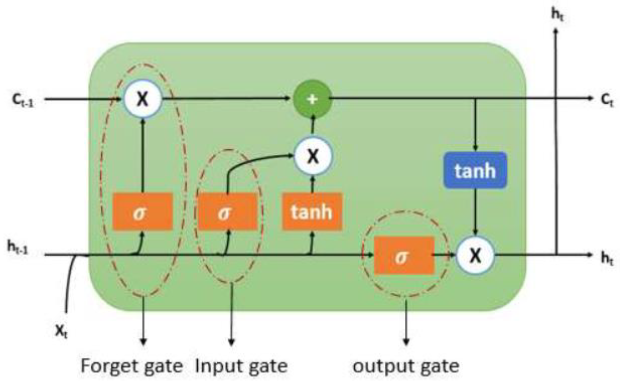
There are input, output, and forget gates in every LSTM cell. The LSTM network store all the data that enters and uses the forget gate to delete information that is not necessary (
Figure 1).
As seen in Figure 1, the preceding hidden state (ht-1), prior cell state (ct-1) and present input (xt) are the inputs of the current cell state (ct). An LSTM cell consists of an input gate, output gate, and forget gate.
The forget gate uses a sigmoid function to identify and decide which information needs to be scrubbed from the block. It examines the previous state (ht-1), the content input (Xt), and each number in the cell state Ct-1 to create a number between 0 (delete) and 1 (store).
An input gate identifies which input value should be utilised to alter the memory. The sigmoid function ascertains whether to permit 0 or 1 values while the tanh function assigns weight to the supplied data and ranks its significance on a scale, from -1 to 1.
An output gate determines the output of a block using its input and memory. The sigmoid function ascertains whether to permit 0 or 1 values while the tanh function ascertains which values, 0 or 1, are permitted to pass through as well assigns weight to the supplied values and ranks their significance on a scale, from -1 to 1, and multiplies it with the sigmoid output.
4.2. LSTM Prediction Algorithm
Long short-term memory (LSTM) is an RNN architecture that is frequently used to predict TSs and process natural language. It can also be used for both univariate and multivariate TS prediction problems.
Univariate LSTMs are used when a TS only contains a single input feature; such as a stock's closing price on a daily basis or a city's temperature on a daily basis. In such cases, the LSTM is trained to forecast future values solely using the single input feature's past values.
Multivariate LSTMs, on the other hand, are used when a TS contains multiple input features; such as a stock's closing price on a daily basis, a city's temperature on a daily basis, and the volume of the stock on a daily basis. In such cases, the LSTM is trained to forecast future values using all these input features' past values.
Regardless of whether an LSTM is univariate or multivariate, the principal idea of its architecture remains the same. Long short-term memory (LSTM) uses gates to control the flow of information through a network as well as preserve dependencies that are long-term in the data. Therefore, LSTMs are ideal and well-suited for TS prediction problems where the correlation between past and future values are complex and may not be easily modelled using traditional statistical methods.
| Univariate LSTM Algorithm |
Multivariate LSTM Algorithm |
1. Libraries Importing and Data Loading: Import the necessary libraries; such as TensorFlow and Numpy; and load the data into the system.
2. Data Pre-processing: Pre-process the data to prepare it for training by removing noise using exponential smoothing (ES), which scales, transforms, and splits the data into training and validation sets.
3. Model Definition: Define the architecture of the LSTM model using the number of units, layers, activation functions, and other hyperparameters.
4. Model Compilation: Compile the model by defining the optimiser, loss function, and metrics to be used.
5. Model Training: Train the model by using the fit() function to fit it to the training data.
6. Model Evaluation: Evaluate the model using the validation dataset and the evaluate() function to calculate performance metrics; such as accuracy and loss.
7. Prediction Generation: Use the model to create predictions using the new data and the predict() function.
8. Results Plotting: Plot the results to visualise the model's performance and compare it to the actual values.
9. Save the Model: Save the trained model to a disc for later use. |
1. Libraries Importing and Data Loading: Import the necessary libraries; such as TensorFlow and Numpy; and load the data into the system.
2. Data Pre-processing: Pre-process the data to prepare it for training by removing noise using ES, which scales, transforms, and splits the data into training and validation sets.
3. Data Reshaping: Reshape the data into a three-dimensional (3D) format with dimensions such as time steps, features, and samples.
4. Model Definition: Define the architecture of the LSTM model using the number of units, layers, activation functions, and other hyperparameters.
5. Model Compilation: Compile the model by defining the optimiser, loss function, and metrics to be used.
6. Model Training: Train the model by using the fit() function to fit it to the training data.
7. Model Evaluation: Evaluate the model using the validation dataset and the evaluate() function to calculate performance metrics; such as accuracy and loss.
8. Prediction Generation: Use the model to create predictions using the new data and the predict() function.
9. Results Plotting: Plot the results to visualise the model's performance and compare it to the actual values.
10. Save the Model: Save the trained model to a disc for later use. |
4.3. Forecast Methods
The data that was used as inputs in this present study was collected from a finance website; namely,
www.investing.com; and used to examine both the univariate and multivariate methods.
4.3.1. Univariate Method Using Closing Prices
As seen in
Figure 2, the performance and price behaviours of the forecasting model were validated by directly inputting the closing prices of a stock.
4.3.2. Multivariate Method Using Closing, Opening, Highest, and Lowest Prices
As seen in
Figure 3, the performance and price behaviours of the forecasting model were validated by directly inputting four different prices of a stock.
Table 4. provides a summary of the statistics of the input data:.
Table 4.
The statistics of the input data obtained from STC, Mobily, and Zain KSA.
Table 4.
The statistics of the input data obtained from STC, Mobily, and Zain KSA.
| Summary Statistics |
STC |
Mobily |
Zain KSA |
| Closing |
Opening |
Highest |
Lowest |
Closing |
Opening |
Highest |
Lowest |
Closing |
Opening |
Highest |
Lowest |
| count |
1462 |
1462 |
1462 |
1462 |
1462 |
1462 |
1462 |
1462 |
1462 |
1462 |
1462 |
1462 |
| mean |
38.58 |
25.29 |
38.92 |
38.25 |
25.29 |
25.29 |
25.56 |
25.01 |
10.85 |
10.85 |
10.98 |
10.73 |
| std |
7.19 |
7.16 |
7.29 |
7.13 |
7.15 |
7.16 |
7.22 |
7.06 |
2.63 |
2.63 |
2.65 |
2.60 |
| min |
26.15 |
13.38 |
26.40 |
26.06 |
13.38 |
13.40 |
13.50 |
13.23 |
5.98 |
5.60 |
6.06 |
5.90 |
| 25% |
33.08 |
19.49 |
33.37 |
32.64 |
19.48 |
19.51 |
19.76 |
19.23 |
8.76 |
8.76 |
8.81 |
8.70 |
| 50% |
39.51 |
24.46 |
39.87 |
39.31 |
24.46 |
24.41 |
24.66 |
24.18 |
11.56 |
11.56 |
11.69 |
11.41 |
| 75% |
43.67 |
30.65 |
44.04 |
43.22 |
30.65 |
30.64 |
30.94 |
30.29 |
13.12 |
13.10 |
13.28 |
12.94 |
| max |
54.48 |
42.88 |
54.74 |
53.93 |
42.88 |
42.92 |
43.43 |
42.30 |
15.13 |
15.13 |
15.20 |
14.99 |
4.4. Noise Removal from the Dataset
The exponential window function is a general method for smoothing TS data, known as exponential smoothing (ES). In contrast to the ordinary moving average, which weights previous data equally, exponential functions use weights that reduce exponentially with time. It is a simple process that can be understood and used to make a decision based on the user's existing presumptions, like seasonality. Time series (TS) data analysis frequently employs ES. One of the various window functions frequently used in signal processing to smooth data is ES, which serves as a low-pass filter to eliminate high-frequency noise.
Poisson's use of recursive exponential window functions in convolutions from the 19th century and Kolmogorov and Zurbenko's use of recursive moving averages in their turbulence studies in the 1940s are methods that precede ES.
The result of the ES algorithm, typically expressed as (Charan et al.), could be viewed as the best prediction of what the next value of (Jarrah & Salim) will be. The raw data sequence is frequently signified by starting at time (t=0). The formulas below provide the simplest form of ES when the observation sequence starts at time (t=0):
Where α is the smoothing factor and 0 < α < 1.
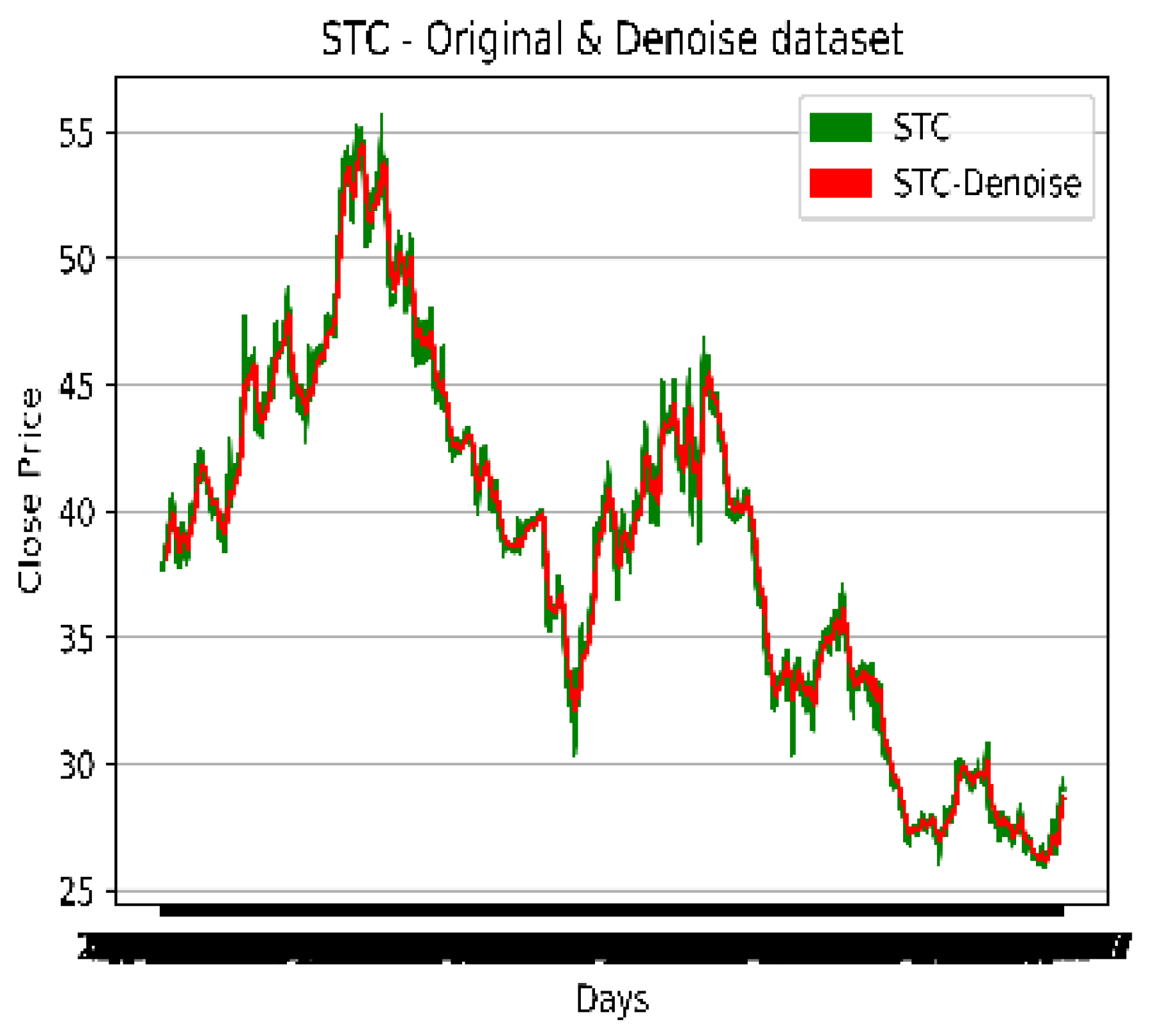
Figure 4,
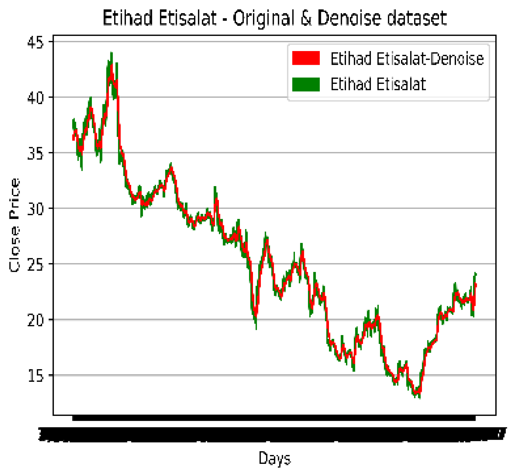
Figure 5 and
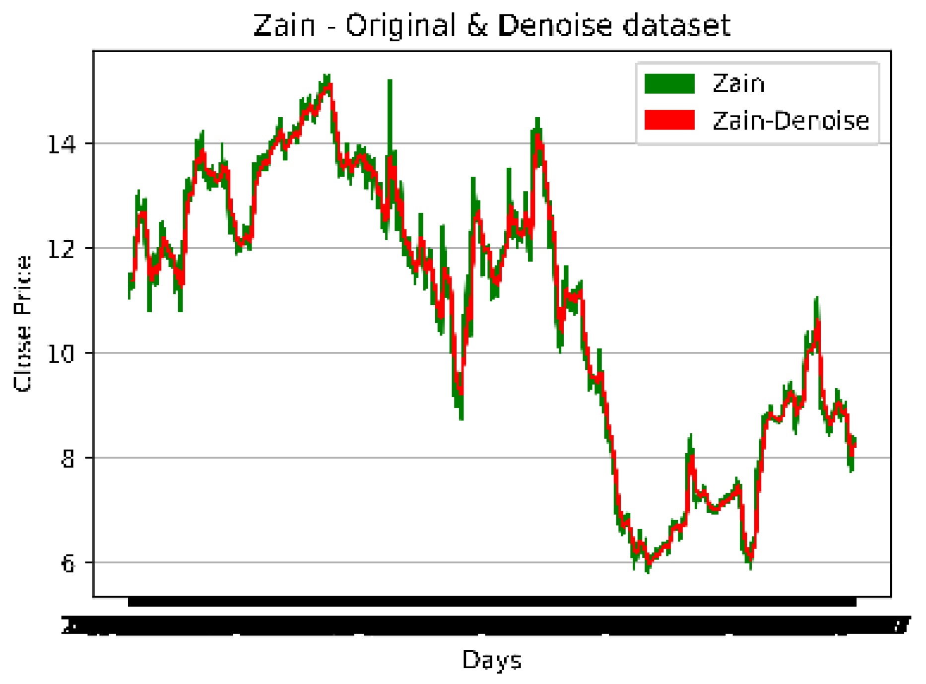
Figure 6 illustrate the importance of showing a sample of the noise in a dataset. The original data was also plotted post-noise removal (denoised). The following figures show the original and denoised datasets.
5. Experiment Results
The present study was conducted using the historical price data of three high volume stocks; namely, STC, Mobily, and Zain KSA; over a period of 1462 days; specifically, from 1 January 2017 to 8 November 2022. Only the closing prices of the aforementioned stocks were used to univariately forecast their closing prices for the subsequent seven days. Meanwhile, four different prices; namely; closing, opening, highest, and lowest; were used to multivariately forecast their closing prices for the subsequent seven days.
5.1. Forecasting Accuracy
Error measures were calculated to assess the feasibility of both the approaches stated in the Methodology and Implementation section. The MAPE, MSE, MAE, and RMSE were employed to substantiate the performance of the suggested models. Equations 8 to 11 depict their formulas. These three indexes are stated as:
where, is the actual value,
is the predicted value, and t = 1…
n and
n are the number of observations.
The outcomes for each of the methods outlined in the Methodology and Implementation section after conducting tests with two different approaches.
5.2. Fitting the Models with LSTM
Similar fitting processes were used for both the univariate and multivariate LSTMs. This involved the following parameters:
Neurons: The quantity of neurons in the network's dense output layer. The number of projected values that a network will generate is determined by the output layer. For instance, in a regression problem, the output layer possesses a single neuron, whereas in a classification problem, the output layer contains the same number of neurons as classes.
Epochs: The number of times that a model will iterate over an entire training dataset. An epoch is defined as one complete iteration over the training data. Although more epochs may increase performance, it also increases the risk of overfitting.
Time steps: The number of time steps or sequence length of the input.
Batch size: The number of samples in a single batch.
Units: The quantity of LSTM units in the layer(s) of the network.
Dropout rate: The rate of dropout regularisation applied to the output of each LSTM unit, which helps prevent overfitting.
Input size: The number of input variables in the input.
Several other parameters; such as the optimiser, loss function, and learning rate; also control the training process and the convergence of a network. Therefore, these parameters must be carefully chosen and tuned according to the specific problem and data at hand.
Table 5. provides a summary of the parameters that were used in the model:.
Table 5.
The parameters of the models.
Table 5.
The parameters of the models.
| |
Univariate LSTM |
Multivariate LSTM |
| Neurons |
32 |
64 |
| Epochs |
150 |
150 |
| Time steps |
10 |
10 |
| Batch size |
32 |
32 |
| Units |
128 |
128 |
| Dropout rate |
0.2 |
0.2 |
| Input size |
1 |
4 |
| Optimiser |
adam |
adam |
5.2.1. The First Method (Univariate)
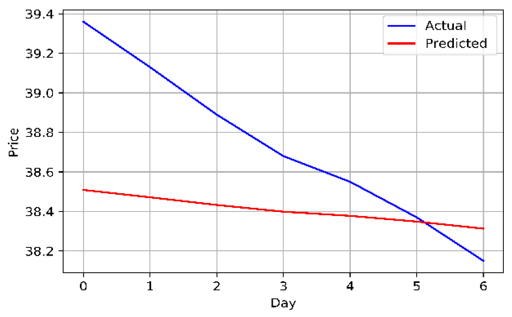
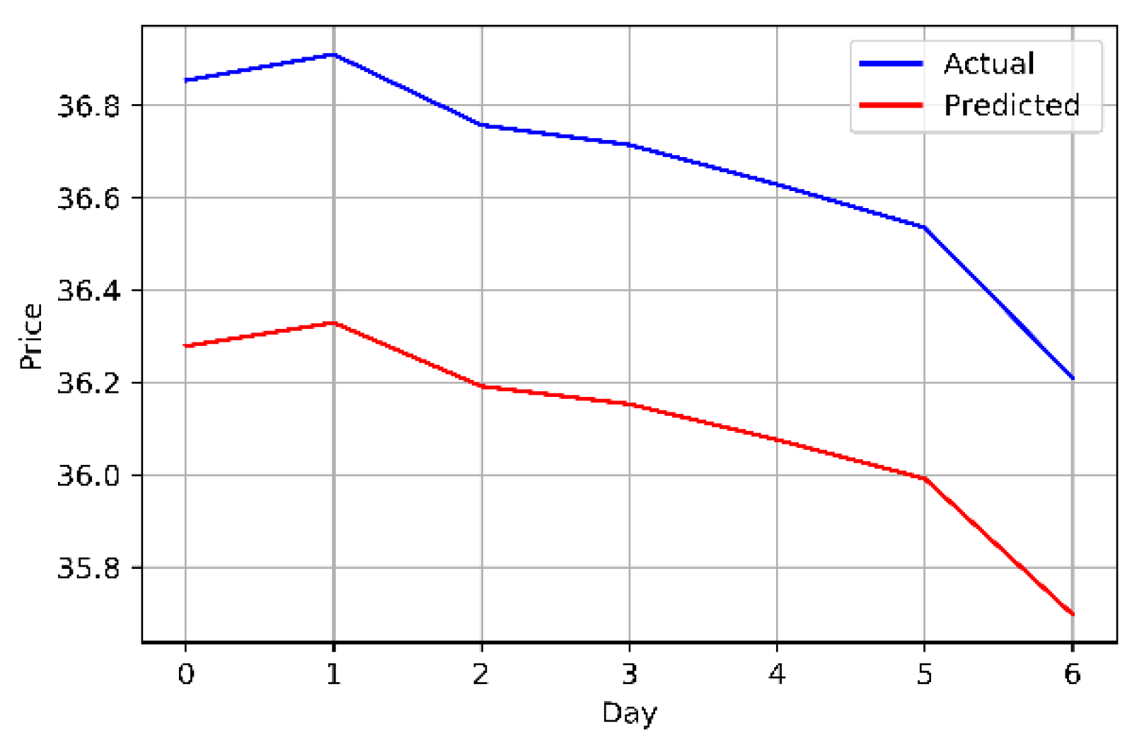
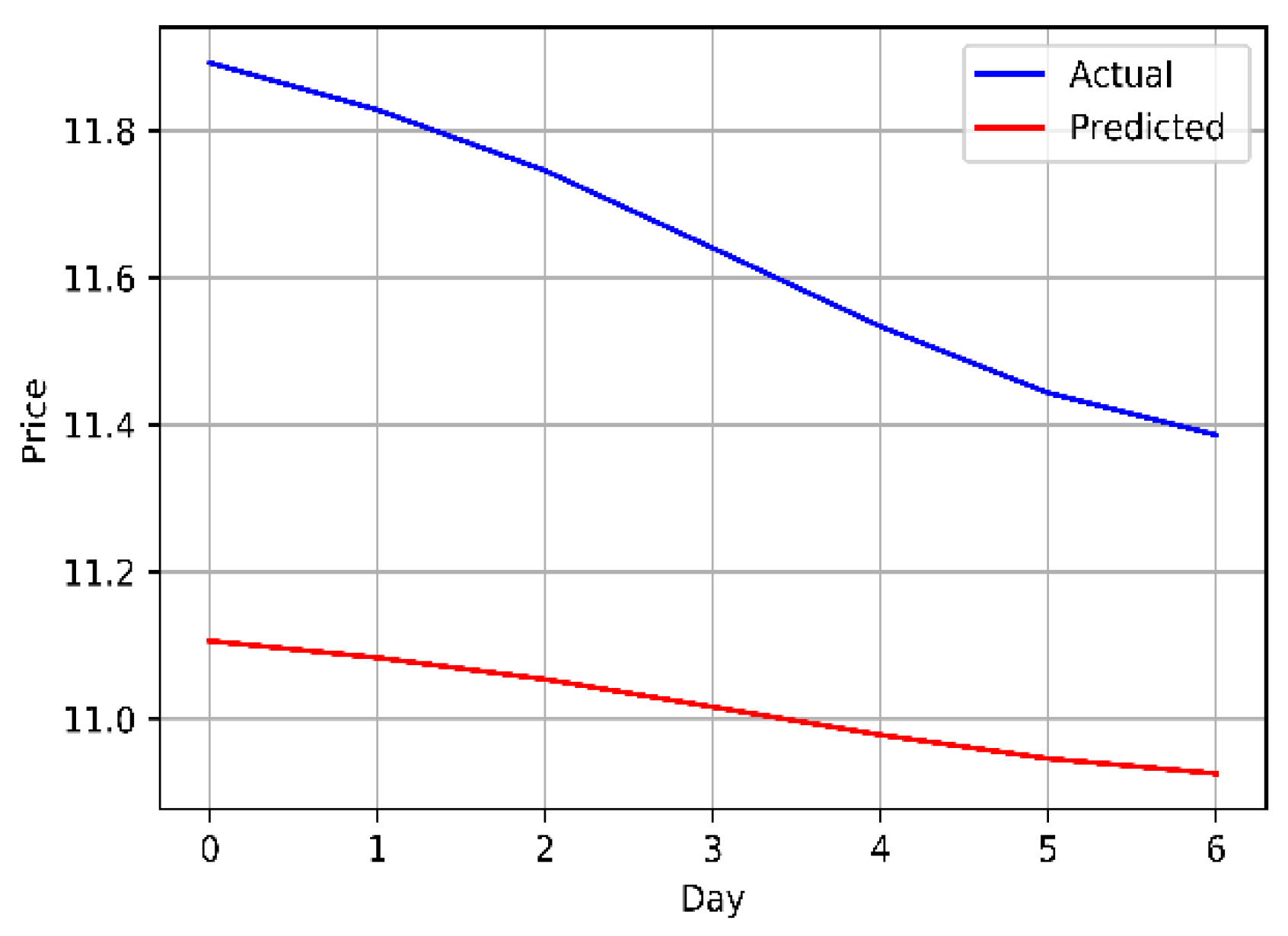
The closing prices of the Mobily, STC, and Zain KSA stocks were fed directly into the LSTM model, which attempts to identify and comprehend patterns in the historic data. As closing price was the only attribute used from the dataset, the model was univariate. Years of historical data was used to train the model.
Table 6 and
Figure 7,
Figure 8 and
Figure 9 provide an explanation of the model's outcomes.
5.2.2. The Second Method (Multivariate)
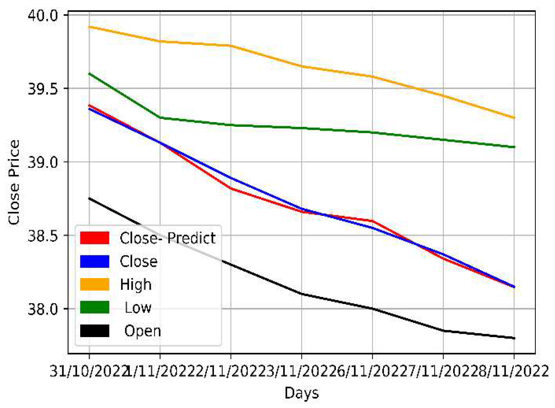
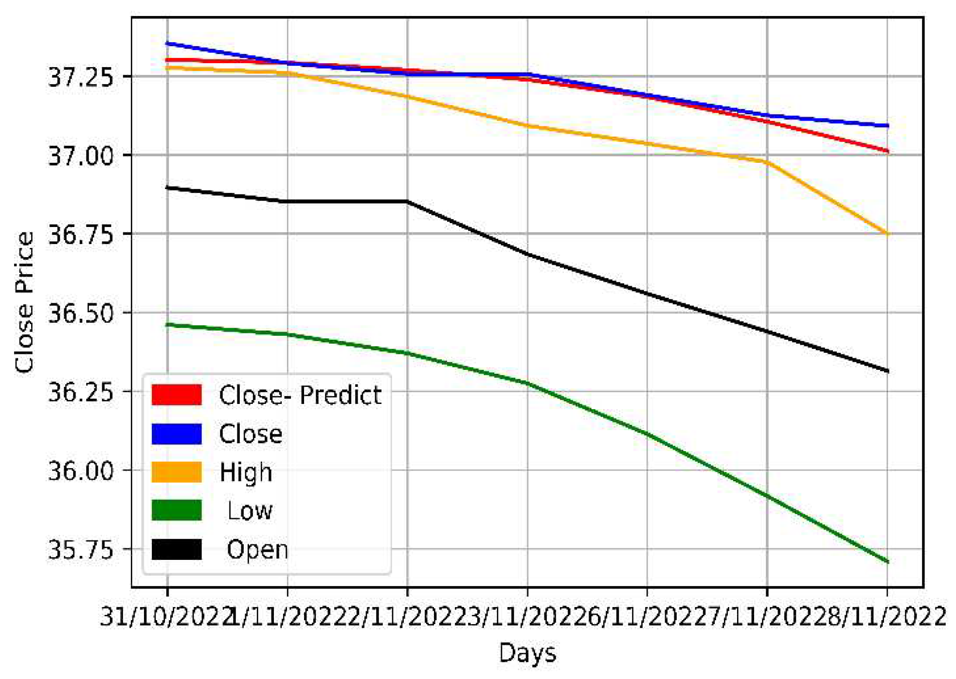
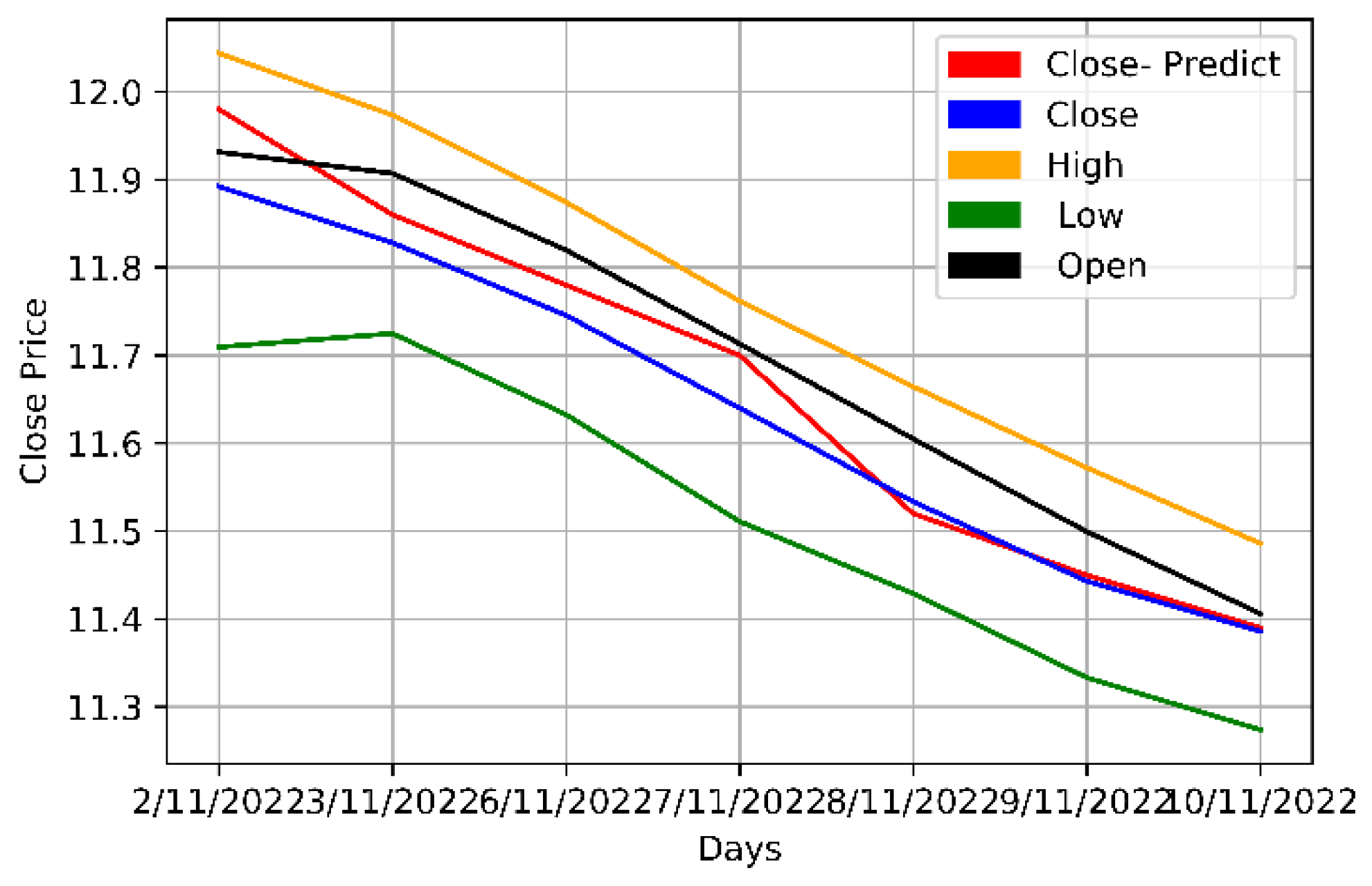
The opening, highest, lowest, and closing prices of the Mobily, STC, and Zain KSA stocks were parallelly fed into the LSTM model. As multiple prices from the dataset were used, the model was multivariate. The model was then trained and its predictions assessed.
Table 7 and
Figure 10,
Figure 11 and
Figure 12 provide a more thorough explanation of the model's outcomes.
The multivariate method, which used multiple stock prices, outperformed the univariate method and successfully predicted the stock prices for the next seven days. The multivariate LSTM models are better at predicting the stock market than their univariate counterparts as they use information from multiple sources; such as the opening, highest, and lowest prices of related stocks; which improves its predictive accuracy. Meanwhile, univariate models only use a single input variable, typically the price of the stock being predicted, which does not contain all the information necessary to make accurate predictions. Furthermore, as multivariate models are also better at capturing the complex correlations and interdependencies of the different input variables, they make significantly more accurate predictions.
6. Conclusions
The purpose of this present study was to forecast stock prices. The stock price performance for the coming week was forecasted using historical data from Mobily, STC, and Zain. The first univariate analysis only applied the closing price data as a single input directly in the LSTMDL projection model while the second multivariate analysis applied the closing, opening, highest, and lowest price data parallelly in the LSTMDL model to forecast the closing prices for the following seven days. The multivariate method predicted the closing prices for the next seven days more accurately than the univariate method, thereby making investments extremely profitable and secure.
Other economic factors; such as governmental regulations, currency exchange rates, interest rates, inflation, Twitter sentiment, or hybrid methods; that influence financial markets may be used to build a knowledge base or as data for forecasting models. Short-term expectations are another variable that could, potentially, affect trend predictions or pricing. This present study only forecasted prices for the following seven days. Therefore, future studies may examine longer periods, such as 10 or 15 days. Long-term predictions may also be examined for further in-depth analysis or guidance. This may include regulatory stability, reviews of quarterly stock performance, sales returns, and dividend returns among other elements. Although longer time frames can be investigated and validated if a longer-term outlook is necessary, shorter time frames; such as the 10-day or 50-day simple moving average (SMA) or exponential moving average (EMA); can also be used.
It is well known that a wide range of aspects; such as governmental regulations, corporate practices, and interest rates to name a few; impact stock prices. For that matter, any announcements regarding these factors impacts stock prices. Even the best ML or DL models will be significantly impacted by natural catastrophes and other unforeseen events. Therefore, a hybrid method that considers all future elements; such as sentiment, news, and technical indicators; can be developed to yield a more vigorous and precise forecasting mechanism.
Acknowledgments
We would like to extend our heartfelt appreciation and gratitude to the Deputyship of the Research & Innovation Department of the Ministry of Education of the Kingdom of Saudi Arabia as well as the Deanship of Scientific Research of the King Abdulaziz University, Jeddah, Kingdom of Saudi Arabia for funding this present study (Project number 528752-G: 243-611-1443).
References
- Alabdulkreem, E., Alruwais, N., Mahgoub, H., Dutta, A. K., Khalid, M., Marzouk, R.,... Drar, S. Sustainable groundwater management using stacked LSTM with deep neural network. Urban Climate 2023, 49, 101469. [CrossRef]
- Charan, V. S., Rasool, A., & Dubey, A. (2022). Stock closing price forecasting using machine learning models. Paper presented at the 2022 International Conference for Advancement in Technology (ICONAT).
- Dinh, T. N. , Thirunavukkarasu, G. S., Seyedmahmoudian, M., Mekhilef, S., & Stojcevski, A. (2023). Predicting Commercial Building Energy Consumption Using a Multivariate Multilayered Long-Short Term Memory Time-Series Model.
- Domala, V., & Kim, T.-W. (2022). A Univariate and multivariate machine learning approach for prediction of significant wave height. Paper presented at the OCEANS 2022, Hampton Roads.
- Jarrah, M. , & Salim, N. (2019). A recurrent neural network and a discrete wavelet transform to predict the Saudi stock price trends. International Journal of Advanced Computer Science and Applications, 10(4).
- Kim, D. , & Baek, J.-G. (2022). Bagging ensemble-based novel data generation method for univariate time series forecasting. Expert Systems with Applications, 203, 117366. [CrossRef]
- Kim, J.-M. , Han, H. H., & Kim, S. (2022). Forecasting Crude Oil Prices with Major S&P 500 Stock Prices: Deep Learning, Gaussian Process, and Vine Copula. Axioms, 11(8), 375.
- Liu, H., & Long, Z. An improved deep learning model for predicting stock market price time series. Digital Signal Processing 2020, 102, 102741. [CrossRef]
- Manujakshi, B., Kabadi, M. G., & Naik, N. A hybrid stock price prediction model based on pre and deep neural network. Data 2022, 7(5), 51. [CrossRef]
- Munkhdalai, L. , Munkhdalai, T., Pham, V.-H., Li, M., Ryu, K. H., & Theera-Umpon, N. Recurrent Neural Network-Augmented Locally Adaptive Interpretable Regression for Multivariate Time-Series Forecasting. IEEE Access, 2022; 10, 11871–11885. [Google Scholar] [CrossRef]
- Nabipour, M., Nayyeri, P., Jabani, H., Mosavi, A., & Salwana, E. Deep learning for stock market prediction. Entropy 2020, 22(8), 840. [CrossRef]
- Tai, C.-Y. , Wang, W.-J., & Huang, Y.-M. Using Time-Series Generative Adversarial Networks to Synthesize Sensing Data for Pest Incidence Forecasting on Sustainable Agriculture. Sustainability, 2023; 15, 7834. [Google Scholar] [CrossRef]
- Thangamayan, S., Kumar, B., Umamaheswari, K., Kumar, M. A., Dhabliya, D., Prabu, S., & Rajesh, N. (2022). Stock Price Prediction using Hybrid Deep Learning Technique for Accurate Performance. Paper presented at the 2022 International Conference on Knowledge Engineering and Communication Systems (ICKES).
- Tuli, S. , Casale, G., & Jennings, N. R. (2022). Tranad: Deep transformer networks for anomaly detection in multivariate time series data. arXiv preprint arXiv:2201.07284.
- Uddin, R., Alam, F. I., Das, A., & Sharmin, S. (2022). Multi-Variate Regression Analysis for Stock Market price prediction using Stacked LSTM. Paper presented at the 2022 International Conference on Innovations in Science, Engineering and Technology (ICISET).
- Youness, J., & Driss, M. (2022). LSTM Deep Learning vs ARIMA Algorithms for Univariate Time Series Forecasting: A case study. Paper presented at the 2022 8th International Conference on Optimization and Applications (ICOA).
- Zaheer, S., Anjum, N., Hussain, S., Algarni, A. D., Iqbal, J., Bourouis, S., & Ullah, S. S. A Multi Parameter Forecasting for Stock Time Series Data Using LSTM and Deep Learning Model. Mathematics 2023, 11(3), 590. [CrossRef]
|
Disclaimer/Publisher’s Note: The statements, opinions and data contained in all publications are solely those of the individual author(s) and contributor(s) and not of MDPI and/or the editor(s). MDPI and/or the editor(s) disclaim responsibility for any injury to people or property resulting from any ideas, methods, instructions or products referred to in the content. |
© 2023 by the authors. Licensee MDPI, Basel, Switzerland. This article is an open access article distributed under the terms and conditions of the Creative Commons Attribution (CC BY) license (http://creativecommons.org/licenses/by/4.0/).
