
Submitted:
17 June 2023
Posted:
20 June 2023
You are already at the latest version
Abstract
Research in brain stroke prediction is very crucial as it can lead to the development of early detection techniques and interventions that can enhance the prognosis for stroke victims. Early detection and intervention can help to minimise the damage caused by a stroke, reduce the risk of long-term complications, and enhance the general quality of life for people who have survived a stroke. Additionally, research in stroke prediction can help to identify risk factors and improve understanding of the underlying causes of stroke, which can lead to the development of better prevention strategies. Research on brain stroke prediction is ongoing and has led to the development of various models and tools for predicting the risk of stroke and detecting it early. However, the implementation and use of these tools in clinical practise vary depending on several factors, such as the availability of resources, the specific healthcare system, and the level of awareness and acceptance of these tools among healthcare providers and patients. In general, risk prediction models may be used to quickly identify individuals at high risk of stroke and target them for preventive interventions, such as lifestyle changes, medication management, and screenings. Early detection tools can be used to quickly identify stroke symptoms and initiate appropriate treatment, which can improve outcomes for stroke patients. However, it is important to note that research and development of these models and tools are ongoing, and their use in clinical practise is constantly evaluated and updated. It may take time for these tools to be widely adopted in clinical practise and to see their real-world impact. This research paper focuses on predicting brain stroke occurrence using a range of machine learning algorithms such as Logistic Regression (LR), Decision Tree (DT), Random Forest (RF), Support Vector Machine (SVM), K-Nearest Neighbor (KNN), Gaussian Naive Bayes (GNB), Bernoulli Naive Bayes (BNB), and a Voting Classifier. The main emphasis of this research was to compare the effectiveness of oversampling techniques, as the data was significantly imbalanced. We have used evaluation metrics in this research to assess the accuracy, precision, recall, and other key performance indicators of a model's predictions. Area under the Receiver Operating Characteristics Curve (AUC), minority class accuracy, and majority class accuracy were used to assess the approaches.
Keywords:
Machine Learning
; Detection
; Prediction
; Oversampling
; SMOTE
1. Introduction
A stroke is a medical emergency requiring immediate medical care when a part of the brain's blood supply is blocked off. A steady supply of oxygen and nutrients is required for the brain to work properly. Even a temporary interruption in blood flow can have serious consequences. When the brain's cells run out of oxygen, they die swiftly. If the damage to the brain is not treated quickly and correctly, it can lead to severe disabilities and even death. The increase in stroke incidence is due to lifestyle, behavioural patterns, demographics (the ageing population), sociocultural factors, and technical improvements. However, the disease can be avoided nearly completely by making some credible and effective corrections to the ways that individuals live their lives. In India, stroke is the 4th major cause of mortality and the 5th greatest cause of disability adjusted life years [1]. Systematic reviews and meta-analyses reveal that the stroke burden in India is quite high. [2]. Brain stroke data can help in medicine by providing information on the causes, risk factors, and patterns of stroke, which can aid in the development of more effective prevention and treatment strategies. Additionally, the use of brain imaging techniques such as MRI and CT scans can assist medical professionals in making a diagnosis and classifying the various types of strokes, which in turn can lead to the selection of treatment options that are suitable. Furthermore, data from clinical trials and observational studies on stroke can be used to improve our understanding of the long-term outcomes and quality of life for stroke survivors and to identify areas for further research.
Most of the existing research on stroke prediction is concerned with a complete and balanced dataset, but few medical datasets can strictly meet such requirements. Prediction of stroke with models of high accuracy has been carried out in the past, but accuracy does not hold true for the imbalanced data. Most of the medical data is incomplete and highly imbalanced, which could lead to a meaningless prediction. In actual clinical practice, the stroke dataset suffers from a class imbalance by nature. In this study, we aim to investigate how to reduce false negatives and false positives and improve mature stroke prediction using the imbalanced dataset. In medical diagnosis, the ideal option for precision and recall would be to have a high value for both metrics. Precision refers to the fraction of true positive predictions among all positive predictions made by the model, while recall refers to the fraction of true positive predictions among all actual positive cases. A high value for precision means that the model has a low rate of false positive predictions, while a high value for recall indicates that the model is able to detect a high proportion of actual positive cases.
To achieve a good balance between precision and recall, various techniques can be used, such as adjusting the threshold for classification, using ensemble models, or employing different algorithms for different subpopulations. However, the best option would depend on the specific context, the characteristics of the dataset, and the trade-off between precision and recall that is acceptable for the particular use case.
2. Related Work
As per the authors [3], the stacking classification method had superior performance, with an AUC of 98.9%, F-measure, precision, and recall of 97.4%, and an accuracy of 98%. This makes it an effective approach for identifying individuals at high risk of experiencing a stroke in the long term. The high AUC values indicate that the model has a strong ability to predict and differentiate between the two classes. Naive Bayes, J48, K-nearest neighbour, and random forest are the four machine learning methods the authors [4] used to accurately predict a stroke. Classifiers such as J48, K-nearest neighbour, and random forest achieved an accuracy of 99.8%, whereas the naive Bayes classifier achieved just 85.6%. In [5], the authors test the ability of multiple ML algorithms to accurately predict stroke based on a variety of physiological factors. Classification accuracy of 96% shows that random forest classification is superior to the other methods tried.
Ref. [6] suggests the application of several machine learning methods, such as logistic regression, decision tree, random forest, K-nearest neighbour, support vector machine and naive Bayes. The naive Bayes, compared to the other algorithms, achieved greater accuracy, with 82% accuracy for the prediction of stroke. In [7] logistic regression, naive Bayes, Bayesian network, decision tree, neural network, random forest, bagged decision tree, voting, and boosting model using decision trees were utilised in order to categorise different degrees of stroke risk. The findings of the experiment revealed that the random forest model achieved the highest level of precision (97.33%), while the boosting model that used decision trees achieved the highest level of recall (99.94%).
Research paper [8] systematically reviews the literature to assess the significance of deep learning techniques in stroke diseases. The findings show that deep learning has a substantial influence on the diagnosis, treatment, and forecasting of strokes. The study also delves into the current limitations and future growth potential of deep learning technology. In this paper, [9] presented a combined machine learning approach incorporating data imputation, feature selection, and prediction. A comprehensive comparison between machine learning methods and the Cox proportional hazards model is provided, demonstrating that machine learning methods outperform the Cox model in both stroke prediction and stroke risk estimation. The conservative mean heuristic is proposed for feature selection, resulting in superior performance compared to other methods. A new prediction algorithm, Margin-based Censored Regression, is introduced, yielding a higher concordance index than the Cox model.
3. Dataset
The Kaggle Dataset [10] is used for this research work. It has 11 variables and 5110 observations. It is very good data, but has a problem that most of the medical data has, i.e. Imbalanced Output Class
No Stroke – 4861
Stroke - 249
Imbalanced datasets have many more instances of certain classes than others [11]. Most machine learning algorithms assume that our datasets have a balanced distribution. As the minority examples occur rarely, rules to predict the small classes are difficult to find. Samples from the minority class are most often misclassified, and we are particularly interested in the minority class.
In real-life, there are many situations where we find imbalanced datasets [12]. Imbalanced datasets are those that have many more instances or observations of a certain class than of other classes. Machine learning algorithms assume that our datasets have a balanced distribution, which means that there are more or less the same number of observations from all the classes that we have in the dataset. The problem when we have few observations of one class that we normally call the “minority class” is that building rules or predictive boundaries to separate the small or minority class from the other classes is exceedingly difficult to find. Therefore, samples from the minority class are most often misclassified as if they were samples from any other class in the majority. Now the problem is that when we work with imbalanced datasets, more often than not we are particularly interested in predicting the minority class. The recurrence of imbalanced datasets in many real-world applications has sparked a huge amount of research in this area. In certain applications, the correct classification of samples in the minority classes often has a greater value than the contrary cases. For example, if we are working with a fraud case and want to identify the fraud instance, that is the one in the minority. The same is true if we are trying to predict a medical diagnosis. This is important because we are usually trying to predict a disease from the records that we have of all the patients. But the prevalence of the disease is usually rare. We are always interested in the positive cases, which are rare, and it is especially important that we get them right so that we can assign the right treatment to the patient. This is what makes working with imbalanced datasets particularly hard, and usually, medical datasets are imbalanced.
4. Methodology for Handling Imbalanced Data
Many medical datasets are imbalanced because the occurrences of certain diseases or conditions are relatively rare, so there may be fewer examples of these in the dataset compared to more common conditions. Additionally, in some cases, data collection may be biased towards certain groups of patients or certain types of treatment, leading to an imbalance in the dataset. Furthermore, some medical datasets may be imbalanced because they are collected from a specific population or geographic region, which may have a different disease distribution than the general population. Furthermore, the imbalance in the dataset may be due to the difficulty or high cost of collecting data on certain diseases, leading to a lack of representation of these diseases in the dataset.
Imbalanced datasets have many more instances of certain classes than of others. Most machine learning algorithms assume that our datasets have a balanced distribution. As the minority examples occur rarely, rules to predict the small classes are difficult to find. Samples from the minority class are most often misclassified, and we are particularly interested in the minority class.
Imbalanced medical datasets can cause a variety of problems when building a prediction model, including:
- Overfitting: Imbalanced datasets can lead to overfitting, where the model performs well on the training data but poorly on unseen data. This is because the model may learn to focus on the majority class and ignore the minority class, leading to poor performance in the minority class. In other words, the model is too specific to the training data and has learned the noise and patterns that are unique to the training set rather than the general underlying patterns that are present in the data. Think of it like a student who has memorized all the answers to a specific test but does not understand the underlying concepts. If the student is given a similar test, they may do very well, but if they are given a different test with new questions, they may struggle. Similarly, in machine learning, a model can be too specific to the training data and have learned the noise and patterns that are unique to the training set, rather than the general underlying patterns that are present in the data. As a result, when the model encounters new data that is not similar to the training data, it may not perform well and make incorrect predictions.
- Biased predictions: Imbalanced datasets can lead to biased predictions, where the model is more likely to predict the majority class, even when the minority class is more likely. Biased predictions are a significant concern in machine learning and data science research. It refers to a situation where machine learning models or algorithms trained on a dataset exhibit systematic and consistent inaccuracies, due to certain biases in the data or model design. Biased predictions can have far-reaching consequences, especially when they are used to make decisions that affect people's lives, such as in healthcare, finance, hiring, and the criminal justice system. If the predictions are based on biased data or models, they can perpetuate and exacerbate existing social and economic disparities and lead to unfair or discriminatory outcomes. Biased predictions can have a significant impact on healthcare, particularly in the areas of diagnosis and treatment. For example, if a machine learning algorithm is trained on a dataset that does not include enough data from certain minority groups or regions, the algorithm may not be able to accurately predict or diagnose illnesses that are more prevalent in those populations. As a result, patients from those groups may be misdiagnosed or receive suboptimal treatment. In addition, machine learning algorithms can also perpetuate biases in healthcare decision-making, such as those related to gender, race, or socioeconomic status. For example, a model that predicts the likelihood of readmission to a hospital may use variables that are correlated with race or socioeconomic status, leading to unfair or discriminatory decisions. This can lead to misdiagnosis or delayed treatment for patients in the minority class.
- Poor performance metrics: Imbalanced datasets can lead to poor performance metrics such as accuracy, precision, and recall, which are commonly used to evaluate the performance of a model. Because these metrics are based on the overall accuracy of the model, they may not accurately reflect the model's ability to correctly predict the minority class.
- Difficulty in comparing models: Imbalanced datasets can make it difficult to compare the performance of different models, as models that achieve high accuracy on an imbalanced dataset may not perform as well on a balanced dataset.
To overcome these issues, there are several techniques that can be used to balance the dataset, such as oversampling [13], undersampling [14], and generating synthetic samples. Additionally, other evaluation metrics, such as the area under the receiver operating characteristic curve (AUC-ROC), can be used to evaluate the model’s performance in an imbalanced dataset. There are several ways to balance a dataset, including:
- Oversampling: The process of increasing the number of samples from the minority class. This involves increasing the number of samples in the minority class by randomly duplicating existing samples [15]. This can help to balance the dataset, but it can also lead to overfitting if the oversampling is not done carefully.
- Undersampling: This involves reducing the number of samples in the majority class by randomly removing samples. This can help to balance the dataset, but it can also lead to a loss of important information if the undersampling is not done carefully.
- Generating synthetic samples: This involves creating new samples for the minority class by combining or modifying existing samples. One popular method is called SMOTE [16](Synthetic Minority Over-sampling Technique) which generates synthetic samples by interpolating between existing minority samples. Other methods include ADASYN (Adaptive Synthetic Sampling) that generates synthetic samples by adjusting the density of the minority class, and Borderline-SMOTE which generates synthetic samples by focusing on samples that are near the decision boundary.
- Using different loss functions: Some loss functions such as Focal Loss, Weighted Cross-Entropy loss, and Dice Loss consider the imbalance of the dataset and adjust the model's weighting of the classes during training.
- Ensemble methods: Ensemble methods like bagging and boosting can also be used to balance the dataset by combining the predictions of multiple models.
- Transfer learning: Pre-training models on a large dataset and then fine-tuning them on a smaller, imbalanced dataset can also be used to balance the dataset.
When using a dataset for building a predictive model for stroke, it is important to make sure that the dataset is representative of the population of interest and that it includes a diverse range of examples. The dataset should include information on the demographic characteristics of the patients, as well as their medical history and laboratory results. It is also important to make sure that the dataset is balanced, as imbalanced datasets can lead to poor model performance and biased predictions. Additionally, it is important to be aware of the possible limitations of the dataset and to use a proper validation strategy to evaluate the model’s performance. It is also important to keep in mind that a model's performance on a specific dataset may not generalize to other populations or settings, and it is important to consider external validation before applying the model in the real world. In this paper, we have used various techniques of oversampling for comparison, as shown in Figure 1. We utilized the imbalanced-learn package [17] in Python to implement resampling techniques.
Oversample (ROS)
Random Over-Sampling (ROS) is a technique used in machine learning to address class imbalance, which occurs when one class of data is significantly more represented in the dataset than the other class(es). It is a simple oversampling technique that addresses class imbalance by randomly duplicating examples from the minority class to balance the dataset. This technique works by randomly selecting examples from the minority class and duplicating them until the number of examples in the minority class is similar to that of the majority class. This ensures that both classes have an equal number of examples, which can lead to better model performance.
Oversample (SMOTE)
SOMTE (Synthetic Minority Over-sampling Technique) [16] is one of the common oversampling techniques that creates new synthetic samples by interpolating between existing minority class samples. Specifically, SMOTE selects a random minority class sample and then identifies its k-nearest minority class neighbours. SMOTE then selects one of these neighbours at random and generates a synthetic sample along the line segment connecting the two points in feature space. The process is repeated until the desired number of synthetic samples is generated. The resulting dataset is then used to train a machine learning model. By oversampling the minority class, the model is able to learn from a more balanced dataset, which can improve the model's ability to predict the minority class accurately. SMOTE is a widely used oversampling technique and is supported by many machine learning libraries and frameworks. This makes it easy to implement and use, and it can be an effective tool for addressing class imbalance in a variety of applications.
Oversample (SMOTENC)
SMOTENC (Synthetic Minority Over-sampling Technique for Nominal and Continuous Features) is an extension of the popular SMOTE algorithm that is specifically designed for datasets that contain both nominal (categorical) and continuous features. SMOTENC is a technique used in machine learning to address class imbalance, where one class of data is significantly more represented in the dataset than the other class(es). In SMOTENC, synthetic samples are generated by selecting a random minority class example and computing the k-nearest neighbours in the feature space. However, unlike SMOTE, SMOTENC considers both the nominal and continuous features when computing the distance between examples. This is important because nominal features cannot be used in traditional distance metrics, and their inclusion in the feature space can lead to biased results. SMOTENC is a powerful technique for addressing class imbalance in datasets with both nominal and continuous features, as it is able to capture the underlying distribution of the minority class more accurately.
Oversample (ADASYN)
ADASYN (Adaptive Synthetic Sampling) [18] is a machine learning technique used to address class imbalance in datasets. Class imbalance occurs when one class of data is significantly more represented in the dataset than the other class(es). It is an extension of the popular SMOTE algorithm, which generates synthetic examples for the minority class to balance the dataset. The ADASYN algorithm works by generating synthetic examples for the minority class in a way that is adaptive to the distribution of the data. Specifically, ADASYN generates synthetic examples for minority class examples that are more difficult to learn by the classifier, by increasing the density of synthetic examples near these difficult examples. The ADASYN algorithm first calculates a density distribution for the minority class examples. It then computes a target density for each example from the minority class based on the ratio of the number of examples in the majority class to the number of examples in the minority class. The target density is higher for minority class examples that are further away from the majority class examples, indicating that they are more difficult to learn. ADASYN is a powerful technique for addressing class imbalance in datasets, as it is able to adapt to the distribution of the data and generate synthetic examples for minority classes that are more difficult to learn.
Oversample (SVM SMOTE)
SVM SMOTE (Support Vector Machine Synthetic Minority Over-Sampling Technique) [19] is a machine learning technique used to address class imbalance in datasets. SVM SMOTE is an extension of the popular SMOTE algorithm, which generates synthetic examples for the minority class to balance the dataset. This algorithm works by first identifying the support vectors for the minority class. Support vectors are examples that are closest to the decision boundary that separates the minority class from the majority class. These support vectors are then used to guide the generation of synthetic examples using the SMOTE algorithm. To generate synthetic examples, SVM SMOTE first selects a minority class example and identifies its k-nearest neighbors in the feature space. It then computes the difference between the minority class example and its nearest support vector and generates a synthetic example by interpolating between the minority class example and one of its k-nearest neighbors, based on the magnitude of this difference. SVM SMOTE is able to generate synthetic examples that are more representative of the minority class distribution and are better suited for training support vector machines, which are a popular algorithm for addressing class imbalance.
Oversample (K Means SMOTE)
K Means SMOTE (K Means Synthetic Minority Over-Sampling Technique) [20] is a machine learning technique used to address class imbalance in datasets. K Means SMOTE is an extension of the popular SMOTE algorithm, which generates synthetic examples for the minority class to balance the dataset. This algorithm works by first clustering the minority class examples into k clusters using the K Means clustering algorithm. K Means clustering is a popular unsupervised learning algorithm that groups similar examples together based on their feature values. Once the minority class examples are clustered, the synthetic examples are generated using the SMOTE algorithm. K Means SMOTE is able to generate synthetic examples that are more representative of the minority class distribution by clustering similar examples together and generating synthetic examples from the mean feature values of each cluster. However, as with any oversampling technique, it is important to carefully evaluate the effectiveness of K Means SMOTE and other oversampling techniques to address class imbalance in a given dataset.
5. Process
The flowchart of the proposed system’s methodology is shown in Figure 2. The dataset for stroke prediction is from Kaggle as mentioned in above section.
Preprocessing
Data Preprocessing is a crucial step in the data analysis and machine learning pipeline, as the quality of the input data can significantly impact the accuracy and effectiveness of the analysis or model. It is the process of cleaning, transforming, and preparing raw data before it is used for analysis or machine learning. It involves a series of steps that aim to enhance the quality of the data and make it more suitable for the analysis or modelling task at hand. The steps involved in data preprocessing can vary depending on the specific dataset and analysis requirements. The steps we have used in this paper are:
- Missing values – Updated the null values of bmi (Body Mass Index) with the mean value.
- Drop ID Column as Stroke is not dependent on this Column.
- Label Encoding - 5 Columns are of Object Type i.e., Gender, ever_married, work_type, Residence_type and Smoking Status. Converted these categorical variables to numerical values, as most machine learning algorithms cannot handle categorical data directly.
- Resample data for handling imbalanced data (We have used seven techniques of Oversampling as mentioned in the Methodology)
- Splitting the data for train and test
- Classification Algorithms
There are several traditional machine learning algorithms that have been used for medical diagnosis using imbalanced data. These include:
- 1)
- Logistic Regression: Logistic Regression [21] is a popular machine learning algorithm used for binary classification problems, where the goal is to predict a binary outcome (e.g., yes/no, true/false). It uses a logistic function to model the probability of a binary outcome based on input features. If the output of the logistic function is greater than 0.5, the prediction is the positive class, and if it is less than 0.5, the prediction is the negative class. Logistic Regression models the relationship between the dependent variable and independent variables as a logistic curve, making predictions in the form of probabilities. These probabilities can then be used as thresholds to make binary class predictions. Logistic Regression is relatively simple to implement, computationally efficient, and can handle a large number of features. The logistic regression algorithm can be extended to handle multiclass classification problems by using one-vs-all or softmax regression. It is widely used in a variety of applications, such as medical diagnosis, credit scoring, image classification, and marketing.
- 2)
- Decision Tree: A Decision Tree is a tree-based machine learning algorithm that works by recursively splitting the data into smaller subsets based on the features that provide the greatest information gain, until the data can be split no further. At each split, a decision is made based on a certain feature, and the data is divided into separate branches, with each branch representing a different outcome. The final result is a tree structure with decision rules at each internal node, and predictions at the leaves. Decision trees are simple, easy to interpret, and can handle both categorical and numerical data. They can be used for both classification and regression tasks. They can handle imbalanced data by adjusting the parameters such as the minimum number of samples required to split a node or create a leaf.
- 3)
-
Random Forest: Random Forest is an ensemble of decision trees; it creates multiple decision trees and combines their predictions to make the final decision. The idea behind this is that multiple trees can work together to overcome the limitations of a single decision tree, such as overfitting, by reducing the variance and increasing the robustness of the model. Random Forest is a powerful and versatile machine learning method that can handle both linear and non-linear relationships, missing values, and large datasets. It is widely used in many applications, such as credit scoring, medical diagnosis, and environmental monitoring.
-
In a Random Forest, information gain is a commonly used criterion for splitting the data at each node of a decision tree. Information gain measures the reduction in entropy (or uncertainty) of the target variable after a split, and the feature that provides the highest information gain is chosen as the splitting feature. The process is repeated recursively until a stopping criterion is met, such as a maximum tree depth or a minimum number of samples in a leaf node.The equation for information gain is as follows:Random forest = Entropy(parent) - (Weighted average) * Entropy(children)where:Entropy(parent) is the entropy of the target variable before the splitEntropy(children) is the entropy of the target variable in each child node after the split(Weighted average) is the weighted average of the entropy of the children, weighted by the size of each child relative to the parent node
- Entropy is a measure of the impurity or disorder of a set of data. In the context of Random Forest, entropy is often used as a criterion to split the data at each node of a decision tree. The goal of the split is to reduce the entropy of the target variable, which in turn increases the purity of the resulting subsets.
-
- 4)
- Support Vector Machine (SVM ): SVM is a supervised learning algorithm that can be used for both classification and regression tasks. SVM can handle imbalanced data by adjusting the class weight parameter, which assigns a higher weight to the minority class. The goal of SVMs is to find the optimal hyperplane that maximally separates the data points of different classes. The hyperplane is chosen such that the margin between the closest data points from each class is maximized. The data points that lie closest to the hyperplane are called support vectors, hence the name "support vector machines".
- 5)
- K-Nearest Neighbors (KNN): KNN is a non-parametric, instance-based learning algorithm. In KNN, the classification of a new data point is determined by the class of its K nearest neighbours in the feature space. The value of K is a hyperparameter that is chosen by the user. Typically, larger values of K result in smoother decision boundaries, while smaller values of K can capture more local details in the data. It can handle imbalanced data by adjusting the number of nearest neighbours, which controls the decision. It can be used for both classification and regression tasks. However, it has some limitations, such as its sensitivity to the choice of distance metric and the curse of dimensionality (i.e., its performance can degrade in high-dimensional spaces). Additionally, KNN requires a large amount of memory to store the entire training dataset for each prediction.
- 6)
- Gaussian Naive Bayes: GaussianNB is a probabilistic algorithm that is commonly used for classification tasks. It is a variant of the Naive Bayes algorithm that makes the assumption that the features are normally distributed, and it is called "naive" because it assumes that the features are independent of each other. It can be used for imbalanced datasets, but its performance may be affected by the degree of imbalance in the data. Like any other classification algorithm, GaussianNB can produce biased results when dealing with imbalanced data, as it is likely to be biased towards the majority class.
- 7)
- Bernoulli Naive Bayes: BernoulliNB is another variant of the Naive Bayes algorithm that is commonly used for binary classification tasks, where the features are binary variables (taking values of either 0 or 1). Bernoulli Naive Bayes is a type of Naive Bayes algorithm that is used for binary classification problems, where the input variables are binary. One of the main advantages of using Bernoulli Naive Bayes is its simplicity and efficiency. It is a fast algorithm that requires relatively little memory and can be easily trained on large datasets. Additionally, it is relatively robust to irrelevant features and noise in the data, making it a good choice for real-world applications. Another advantage of Bernoulli Naive Bayes is that it can handle high-dimensional datasets with ease. This is because it models the conditional probability of each feature given the class label separately, allowing it to handle a large number of features without requiring a large amount of training data. Overall, Bernoulli Naive Bayes is a powerful and widely-used algorithm that is particularly useful for binary classification problems, such as text classification. It is fast, efficient, and robust, making it a good choice for real-world applications with large datasets. Bernoulli Naive Bayes (BernoulliNB) can handle imbalanced data to some extent, but its performance may be limited if the dataset is severely imbalanced.
- 8)
- Voting Classifier: The voting classifier [22] is an ensemble learning method that combines the predictions of multiple base models to make a final prediction. Voting Classifier is a type of ensemble learning technique in which multiple models (classifiers) are combined to improve the performance of the overall system. It works by aggregating the predictions of multiple base classifiers and combining them into a single prediction. The main reason for using a Voting Classifier is to improve the overall accuracy and robustness of the model. By combining multiple models, the Voting Classifier can reduce the risk of overfitting and bias that can occur when using a single model. Another advantage of using a Voting Classifier is that it can handle different types of models. For example, you can combine the predictions of a logistic regression model, a decision tree model, and a random forest model into a single prediction. This can be particularly useful when you have different types of data or when different models perform better on different subsets of the data. Overall, the Voting Classifier is a powerful technique that can help improve the accuracy and robustness of your model and is particularly useful when dealing with complex data or when you have a variety of models to choose from. In our case, we are considering combining Logistic Regression, Decision Tree, Random Forest (Information Gain), Random Forest (Entropy), Support Vector Machine, K-Nearest Neighbors, Gaussian Naive Bayes, and Bernoulli Naive Bayes using a voting classifier.
The right validation techniques help to estimate unbiased generalized model performance and give a better understanding of how the model was trained. While the choice of the algorithms might have some impact on the classification results for imbalanced data, the choice of the technique for handling imbalanced data is more critical. A number of approaches have been developed throughout the years to work with imbalanced datasets and try to build better-performing machine learning models and different approaches work better in different scenarios. These approaches can be grouped broadly into three groups - the data level approaches, the cost sensitive approaches and the ensemble algorithms approaches [23]. Data level approaches will modify the dataset, cost sensitive approaches will modify the cost that we are trying to optimize and ensemble algorithms will leverage the power of building several algorithms to predict the minority class in an imbalance dataset. Among the data level approaches, the main approaches have focused on undersampling and oversampling the dataset. Data level approaches refer to changing the distribution of the data in general to have more observations from the minority class or less observations from the majority class so that we reach a similar ratio from each one of the classes. We have approaches like random oversampling and random undersampling, which increase the number of observations from the minority or decrease the number of observations from the majority at random.
When dealing with imbalanced datasets, where one class has many more examples than the other, the model may be biased towards the majority class, leading to a higher number of false negatives or false positives. There are several methods that can be used to reduce false positives and false negatives in imbalanced datasets:
- i.
- Resampling techniques: Techniques such as oversampling the minority class, undersampling the majority class, or using a combination of both, called SMOTE (Synthetic Minority Over-sampling Technique), can be used to balance the data and reduce the false negatives and false positives.
- ii.
- Change the threshold: The threshold of a classification model is the point at which predictions are classified as positive or negative. By adjusting the threshold, one can either increase the recall of the model at the expense of precision or increase the precision of the model at the expense of recall.
- iii.
- Ensemble models: Combining multiple models can help reduce false negatives and false positives by averaging their predictions and reducing the variability in their results.
- iv.
- Cost-sensitive learning: Assign different costs to different types of misclassification errors and adjust the model's learning algorithm to minimize the overall cost.
- v.
- Anomaly detection techniques: Utilizing techniques such as clustering, density-based methods and isolation forest can help in reduce false positives and false negatives.
- vi.
- Using different models: Using models such as Random Forest, XGBoost and LightGBM, can also help reduce false positives and false negatives.
- vii.
- Hyperparameter tuning: Optimizing the model's hyperparameters, such as learning rate and regularization strength, can help improve its performance and reduce false positives and false negatives.
6. Results and Analysis
In medical diagnosis, false negatives are generally considered to be more concerning than false positives. A false negative result means that the model has incorrectly diagnosed a patient as not having a disease when they actually do. This can lead to delayed treatment, which could make the patient's situation even worse. On the other hand, a false positive result means that the model has incorrectly diagnosed a patient as having a disease, when they actually do not. This can cause unnecessary stress, testing, and treatment for the patient. That being said, the "better" option between false positives and false negatives can depend on the specific context and the consequences of each type of error. It is important to weigh the trade-offs and make informed decisions to optimize the model's performance for a specific use case. Precision alone is not a sufficient measure of a model's performance and should be considered alongside other metrics such as recall and F1 score. Unfortunately, you cannot have it both ways; increasing precision means decreasing recall, and vice versa. This kind of compromise is referred to as the “precision-recall trade-off”.
In binary classification problems, commonly used evaluation metrics include accuracy, precision, recall, F1-score, and ROC curve. These metrics are used to compare different models and suggested the best one for a given problem. Evaluation metrics are important because they help us to determine how well a model is performing and whether it is meeting our expectations. By comparing the model's predicted output to the actual output, we can identify any patterns of error and work to enhance the model's performance.
- Precision: In terms of all positive predictions (TP + FP), precision is the percentage of true positive predictions (TP) among all positive predictions. In other words, precision measures how often the model correctly identifies positive instances. High precision means that the model makes very few false positive predictions. This is useful when the cost of false positives is high (e.g., in medical diagnosis, predicting a condition that does not exist).
- Recall: Recall counts the percentage of accurate positive predictions (TP) among all instances of positive data (TP + false negative predictions (FN)). In other words, recall measures how often the model correctly identifies actual positive instances. High recall means that the model is able to correctly identify most of the actual positive cases. This is useful when the cost of false negatives is high (e.g., in medical diagnosis, missing a disease that exists).
- F1-score: The F1-score is the harmonic mean of precision and recall, giving equal weight to both metrics. It provides a single value that summarizes the model's performance, with 1 being the best possible value and 0 being the worst possible value. The F1 score is a good metric to use when the goal is to balance precision and recall, it is the harmonic mean of precision and recall, which gives more weight to the lower value, this means that if either precision or recall is low, the F1 score will be low as well. In cases where the dataset is balanced, precision and recall have similar importance, so the F1 score is a useful metric to assess the model’s performance. However, when the dataset is imbalanced, it could be more important to have higher precision or higher recall, depending on the cost of false positives/false negatives. In those cases, it is important to consider both precision and recall as well as the F1 score. The F1 score is especially helpful when the distribution of classes in the dataset is imbalanced, which is a common scenario in many real-world applications.
- Support: Support refers to the number of instances belonging to each class in the dataset. Support is important to consider in model evaluation because it helps in providing the context for the performance metrics. For example, if the precision for a class is very high but the support is very low, it may not be very meaningful because there are only a few instances of that class. On the other hand, if the precision is high and the support is also high, it implies that the model is doing well on a larger number of instances in that class.
- Accuracy: Accuracy measures the proportion of correct predictions among all predictions made by the model.
- A confusion matrix is a table that is often used to describe the performance of a classification algorithm. It is a table with four different rows and columns that reports the number of true positives (TP), false positive (FP), true negative (TN), and false negative (FN). The importance of a confusion matrix in model evaluation is that it allows one to see how well the model can correctly predict or classify the different classes. It also provides insights into the types of errors that the model is making, which can be useful for further improving the model. Additionally, it allows for the calculation of various performance metrics, such as precision, recall, and F1 score, which can be used to compare the performance of different models.
Following are the results of the various machine learning models that have been used in this paper. The first model is created using the original data, which is highly imbalanced and referred to as the baseline model. Establishing a baseline is important in machine learning, as it helps to determine the effectiveness of new models or techniques and to identify whether the improvement in performance is significant or not. Without a baseline, it can be difficult to assess the performance of new models or techniques and to determine if they are worth pursuing further. A baseline is a reference point or starting point against which, something can be measured, evaluated, or compared. It is often used as a benchmark or standard to assess the performance of a system or process. In the context of machine learning, a “baseline” is the performance of a simple, well-established model or method that serves as a reference point for comparison to more complex or novel models. In this research, for the baseline model, we have used the imbalanced dataset as it is. Other models have used oversampling techniques ROS, SMOTE, SMOTENC, ADASYN, SVM SMOTE and K Means SMOTE respectively and results are as follows:
Baseline (Without any Sampling): The given metrics (Classification Report and Confusion Matrix) in Figure 3 suggest that this baseline model has achieved high precision and recall for class 0 (with a precision of 0.95 and a recall of 1.0). However, for class 1, the precision and recall are both 0, which indicates that the model has not correctly identified any instances of this class. For a binary classification problem, the ROC curve plots the true positive rate (TPR) to the false positive rate (FPR) at different threshold settings. Since the given confusion matrix has only two predicted classes, we can calculate TPR and FPR as follows:
TPR = true positives / (true positives + false negatives) = 0 / 50 = 0
FPR = false positives / (false positives + true negatives) = 0 / 972 = 0
As TPR and FPR are both 0, the ROC curve for this matrix will consist of only one point at the bottom left corner of the plot, indicating that the model does not distinguish between the two classes. Therefore, the AUC (area under the ROC curve) will be 0.5, which is equivalent to random guesswork. In summary, the ROC curve for this confusion matrix suggests that this model has poor performance and does not distinguish between the two classes. Further investigation needs to be done to find out the potential ways to improve the model's performance. It is important to remember that enhancing a model's performance is an iterative process that may involve experimenting with various strategies and modifying parameters until the desired performance is attained.
Oversample (ROS): In this case of random over sampling (ROS), the given confusion matrix and classification report in Figure 4 suggest that the model has achieved high precision and recall for both classes, with a weighted average F1-score of 0.94. However, there is a noticeable difference in precision and recall between the two classes, with class 0 having a slightly lower recall (0.92) compared to class 1 (0.96). The ROC curve for this confusion matrix suggests that the model has good performance, with an AUC of 0.96. The curve is closer to the top-left corner, which indicates a higher TPR at a lower FPR. This means that the model can distinguish between the two classes effectively. Overall, the ROC curve supports the classification report's conclusion that the model has performed well.
Oversample (SMOTE): Looking at the confusion matrix and the classification report, the model has an accuracy of 0.91, with precision of 0.92 and 0.89 for class 0 and class 1, respectively. The recall is 0.88 for class 0 and 0.93 for class 1. The precision and recall scores for both classes are also quite good, indicating that the model is able to correctly classify both positive and negative samples. The F1-score is 0.90 for class 0 and 0.91 for class 1. As we can see in Figure 5, the ROC curve is quite good, with an AUC value of 0.92, indicating a strong performance of the classification model.
Oversample (SMOTENC): Based on the given metrics and confusion matrix in Figure 6, the model appears to perform well with high precision, recall, and f1-score for both classes, as well as high accuracy. The confusion matrix also shows a relatively small number of false positives and false negatives. Therefore, the ROC curve is expected to show a high true positive rate and a low false positive rate, resulting in a curve that approaches the upper left corner of the graph, which is the ideal position for a binary classifier. The ROC curve shows that the model has a high true positive rate (TPR) and a low false positive rate (FPR), indicating that the model is performing well. The AUC value of 0.94 also indicates good model performance.
Oversample (ADASYN): The model has an overall accuracy of 0.91, which indicates that it is correctly predicting the class labels for the majority of instances in Figure 7. The precision and recall values for class 0 and class 1 are fairly balanced, with slightly higher precision for class 0 and slightly higher recall for class 1. The F1-scores for both classes are also high, indicating good performance. Looking at the confusion matrix, we can see that the model is precisely identifying a large number of instances in both classes, with only a relatively small number of false positives and false negatives. However, it is misclassifying slightly more instances from class 1 as class 0 (63) compared to the other way around (103). Overall, the model appears to be performing well, but there may be some room for improvement, particularly in reducing the number of false negatives for class 1. Further analysis could be done to investigate potential ways to improve the model's performance, such as by adjusting the decision threshold or trying different modelling techniques.
Based on the ROC analysis, the model seems to have good predictive power with an AUC of 0.93. The ROC curve shows that the model has a high true positive rate (TPR) for most of the range of false positive rate (FPR), indicating that it is able to correctly classify a large proportion of positive cases while keeping the false positive rate relatively low. However, the steepness of the curve at the beginning indicates that the model may have a relatively high false positive rate at low thresholds. Overall, the ROC analysis suggests that the model is a good performer, but further evaluation and optimization may be necessary to improve its performance.
Oversample (SVM SMOTE): Based on the provided classification report in Figure 8, the precision for class 0 (0.95) is higher than that of class 1 (0.87), indicating that the model performs better at identifying negative instances (class 0) compared to positive instances (class 1). However, the recall for class 1 (0.92) is higher than that of class 0 (0.92), indicating that the model has a better ability to identify positive instances. The F1-score, which balances precision and recall, is higher for class 0 (0.93) than for class 1 (0.90).
In summary, the model has a higher precision for negative instances but a higher recall for positive instances. It has an overall accuracy of 0.92 and performs relatively well at identifying both positive and negative instances, but there is still room for improvement in reducing the number of false positives and false negatives. The ROC curve for the given model looks good, as the AUC is 0.94, which indicates that the model is able to distinguish between positive and negative classes effectively.
Oversample (K Means SMOTE): As shown in Figure 9, the model has an overall accuracy of 96%, with a precision of 95% for predicting class 0 and a precision of 97% for predicting class 1, which indicates that it is performing well. The precision and recall scores for both classes are also high, indicating that the model is able to correctly classify both classes with a high degree of accuracy. The F1-score, which is the harmonic mean of precision and recall, is also high for both classes. The confusion matrix shows that there are a small number of false positives and false negatives, indicating that the model is doing a good job of balancing the trade-off between precision and recall.
Overall, based on these metrics, the model appears to be performing very well on this particular dataset. The ROC curve for the given model has an AUC of 0.97, which indicates excellent discrimination between positive and negative classes. The ROC curve shows that the model has a high true positive rate (TPR) with low false positive rate (FPR) values, indicating that the model is effective in identifying true positives while minimizing false positives. The ROC curve is almost at the top-left corner of the plot, indicating that the model has high sensitivity and specificity. Overall, the model appears to have particularly good performance based on the ROC curve analysis.
Table 1 represents the performance metrics of various techniques used for a classification task, with accuracy, false positives, false negatives, and ROC as evaluation metrics. The techniques are compared against a baseline with an accuracy of 95%, no false positives, and 50 false negatives, resulting in an ROC score of 0.5. The following are the observations we can make based on the table:
- i.
- The ROS (Random Over-Sampling) technique has a slightly lower accuracy of 94% compared to the baseline, but it significantly reduces false negatives to 43, resulting in a higher ROC score of 0.96. However, it comes at a cost of 72 false positives.
- ii.
- The SMOTE (Synthetic Minority Over-sampling Technique) technique has an even lower accuracy of 91% compared to the baseline, with a high number of false positives and false negatives, resulting in an ROC score of 0.92.
- iii.
- The SMOTENC (SMOTE for Nominal and Continuous) technique has a slightly better accuracy of 92% compared to SMOTE, with a lower number of false positives and false negatives, resulting in a higher ROC score of 0.94.
- iv.
- The ADASYN (Adaptive Synthetic) technique has a similar performance to SMOTENC, with an accuracy of 91%, a moderate number of false positives and false negatives, and an ROC score of 0.93.
- v.
- The SVM SMOTE (Support Vector Machine SMOTE) technique has a similar performance to SMOTENC and ADASYN, with an accuracy of 92%, a low number of false positives and false negatives, and an ROC score of 0.94.
- vi.
- The K Means SMOTE technique has the highest accuracy of 96% among all techniques, with a low number of false positives and false negatives, resulting in the highest ROC score of 0.97.
Overall, the K Means SMOTE technique seems to perform the best among the techniques listed, with the highest accuracy and ROC score. However, the choice of technique may depend on the specific requirements of the task, such as the cost of false positives and false negatives and the size of the dataset. False negatives in medical diagnosis can occur when a disease or condition is present but is not detected by the diagnostic test. This is particularly concerning in medical diagnosis because missing a disease that exists can have serious consequences for the patient. In these cases, the cost of missing something relevant is high, and as a result, reducing false negatives is crucial. False positives in medical diagnosis can occur when a disease or condition is not present but is detected by the diagnostic test. This can lead to unnecessary treatment, anxiety, and potential harm to the patient. While false positives can be an issue in medical diagnosis, they are generally less concerning than false negatives in this context. This is because false positives typically result in additional testing or observation rather than the withholding of necessary treatment. However, in some cases, false positives can lead to unnecessary treatment, which can be costly and potentially harmful to the patient. There are several reasons why false negatives or positives may occur in medical diagnosis:
- Limited specificity of diagnostic tests: Some diagnostic tests may have a lower specificity, which means they may detect a disease even when it is not present. This can lead to false negatives or positives.
- Disease manifestation: Some diseases may have a very non-specific presentation, making it difficult to differentiate from other conditions.
- Limited access to medical facilities: In some locations, patients may not have access to advanced medical facilities or experienced medical professionals, which can lead to false negatives or positives.
- Limited availability of diagnostic tests: Some diagnostic tests may not be widely available, especially in resource-limited settings, which can lead to false negatives or positives.
- Patient's characteristics: Some patient's characteristics, such as age, sex, or other underlying medical conditions, can affect the diagnostic test's results, leading to false negatives or positives.
- Human error: False negatives or positives can also occur due to human error, such as misinterpreting test results or not conducting the test properly.
It is important to note that false positives are not only a problem in medical diagnosis, but also in other fields such as fraud detection, cybersecurity and anomaly detection. In these cases, the cost of investigating something that is not relevant is high, and as a result, reducing false positives is crucial. Similarly, false negatives also occur in other fields such as fraud detection, cybersecurity, or anomaly detection and need to be reduced.
7. Conclusion
Due to the imbalanced nature of the data in real-world scenarios, we were facing challenges to get exact predictions for problems like credit card fraud, cyclone data, equipment testing and production, the detection of oil spills from radar photos of the ocean, and medical diagnosis. This research work on the use of oversampling methodology is a step in the right direction to forecast the pattern and evaluation of the minority class so that an efficient method of analysis can be offered to make the prediction accurately. The paper discusses the different models used for early detection of stroke using various machine learning algorithms such as logistic regression, decision trees, random forests, support vector machines, K-nearest neighbour, Gaussian naive bayes, Bernoulli naive bayes, and a voting classifier. It should be acknowledged, however, that these models' effectiveness in real-world healthcare environments continues to be investigated and enhanced.
One potential idea for handling imbalanced data in medical diagnosis that has not been widely used yet is the use of Generative Adversarial Networks (GANs) to generate synthetic samples of the minority class. GANs are neural networks that can generate new data that is similar to the training data. In the context of medical diagnosis, GANs could be trained on a small dataset of cases of a rare disease and then used to generate synthetic samples that could be added to the dataset to improve the performance of the classifier. This approach could be useful in situations where there is limited data available for a rare disease, and it would allow for the creation of a larger and more balanced dataset without the need for manual annotation or data collection. Another idea is to use active learning techniques to actively select the most informative samples from the dataset to train the model. Active learning is a machine learning paradigm where the model is able to query the human expert in order to decide which data to use for training. This can help in cases where there is a small sample of cases for the rare disease, and the model will have a better chance of generalizing to unseen cases. It is important to note that these are just ideas, and they have not been widely used or tested in medical diagnosis. Before putting them into clinical practice, it is crucial to assess their efficacy and reliability.
References
- NPCDCS, “Guidelines for prevention and management of stroke,” Natl. Program. Prev. Control Cancer, Diabetes, Cardiovasc. Dis. Stroke (NPCDCS), Gov. India Guidel. Prev. B. C. V, Silva, D. A. De, Macleod, M. R., Coutts, S. B., Schwamm, L. H., Davis, S. M., D, no. 61, pp. 1–16, 2019. [CrossRef]
- S. Khurana, M. Gourie-Devi, S. Sharma, and S. Kushwaha, “Burden of Stroke in India during 1960 to 2018: A Systematic Review and Meta-Analysis of Community Based Surveys,” Neurol. India, vol. 69, no. 3, pp. 547–559, 2021. [CrossRef]
- E. Dritsas and M. Trigka, “Stroke Risk Prediction with Machine Learning Techniques,” Sensors, vol. 22, no. 13, 2022. [CrossRef]
- T. I. Shoily, T. Islam, S. Jannat, S. A. Tanna, T. M. Alif, and R. R. Ema, “Detection of Stroke Disease using Machine Learning Algorithms,” 2019 10th Int. Conf. Comput. Commun. Netw. Technol. ICCCNT 2019, pp. 1–6, 2019. [CrossRef]
- T. Tazin, M. N. Alam, N. N. Dola, M. S. Bari, S. Bourouis, and M. Monirujjaman Khan, “Stroke Disease Detection and Prediction Using Robust Learning Approaches,” J. Healthc. Eng., vol. 2021, pp. 1–12, 2021. [CrossRef]
- G. Sailasya and G. L. A. Kumari, “Analyzing the Performance of Stroke Prediction using ML Classification Algorithms,” Int. J. Adv. Comput. Sci. Appl., vol. 12, no. 6, pp. 539–545, 2021. [CrossRef]
- X. Li, D. Bian, J. Yu, H. Mao, M. Li, and D. Zhao, “Using machine learning models to classify stroke risk level based on national screening data ∗,” Proc. Annu. Int. Conf. IEEE Eng. Med. Biol. Soc. EMBS, vol. 2, pp. 1386–1390, 2019. [CrossRef]
- S. Zhang et al., “Research Progress of Deep Learning in the Diagnosis and Prevention of Stroke,” Biomed Res. Int., vol. 2021, 2021. [CrossRef]
- Khosla, Y. Cao, C. C. Y. Lin, H. K. Chiu, J. Hu, and H. Lee, “An integrated machine learning approach to stroke prediction,” Proc. ACM SIGKDD Int. Conf. Knowl. Discov. Data Min., pp. 183–191, 2010. [CrossRef]
- Fedesoriano, “Stroke Prediction Dataset,” Kaggle, 2021. https://www.kaggle.com/datasets/fedesoriano/stroke-prediction-dataset (accessed Apr. 14, 2023).
- G. M. Weiss, “Foundations of imbalanced learning,” in Imbalanced Learning: Foundations, Algorithms, and Applications, John Wiley & Sons, Ltd, 2013, pp. 13–41. [CrossRef]
- Y. Sun, A. K. C. Wong, and M. S. Kamel, “Classification of imbalanced data: A review,” Int. J. Pattern Recognit. Artif. Intell., vol. 23, no. 4, pp. 687–719, 2009. [CrossRef]
- “Over-sampling methods.” https://imbalanced-learn.org/dev/references/over_sampling.html (accessed Apr. 14, 2023).
- “Under-sampling methods,” imbalanced-learn Dev., 2022, Accessed: Apr. 14, 2023. [Online]. Available: https://imbalanced-learn.org/dev/references/under_sampling.html.
- R. Mohammed, J. Rawashdeh, and M. Abdullah, “Machine Learning with Oversampling and Undersampling Techniques: Overview Study and Experimental Results,” 2020 11th Int. Conf. Inf. Commun. Syst. ICICS 2020, pp. 243–248, 2020. [CrossRef]
- N. V. Chawla, K. W. Bowyer, L. O. Hall, and W. P. Kegelmeyer, “SMOTE: Synthetic Minority Over-sampling Technique Nitesh,” J. Artif. Intell. Res., vol. 30, no. 2, pp. 321–357, 2002. [CrossRef]
- G. LemaˆıtreLemaˆıtre, F. Nogueira, and C. K. Aridas char, “Imbalanced-learn: A Python Toolbox to Tackle the Curse of Imbalanced Datasets in Machine Learning,” J. Mach. Learn. Res., vol. 18, pp. 1–5, 2017, Accessed: Apr. 16, 2023. [Online]. Available: http://jmlr.org/papers/v18/16-365.html.
- H. He, Y. Bai, E. A. Garcia, and S. Li, “ADASYN: Adaptive synthetic sampling approach for imbalanced learning,” in Proceedings of the International Joint Conference on Neural Networks, 2008, pp. 1322–1328. [CrossRef]
- H. Sain and S. W. Purnami, “Combine Sampling Support Vector Machine for Imbalanced Data Classification,” in Procedia Computer Science, 2015, vol. 72, pp. 59–66. [CrossRef]
- F. Last, G. Douzas, and F. Bacao, “Oversampling for Imbalanced Learning Based on K-Means and SMOTE,” 2017. [CrossRef]
- “Logistic Regression.” https://www.sciencedirect.com/topics/medicine-and-dentistry/multivariate-logistic-regression-analysis (accessed Apr. 16, 2023).
- “Voting Classifier.” https://scikit-learn.org/stable/modules/generated/sklearn.ensemble.VotingClassifier.html (accessed Apr. 16, 2023).
- D. Kanellopoulos, S. Kotsiantis, and P. Pintelas, “Handling imbalanced datasets: A review Cite this paper Related papers Handling imbalanced datasets: A review,” GESTS Int. Trans. Comput. Sci. Eng., vol. 30, no. 1, pp. 25–36, 2006.
Figure 1.
Techniques for Balancing the Imbalanced Dataset.
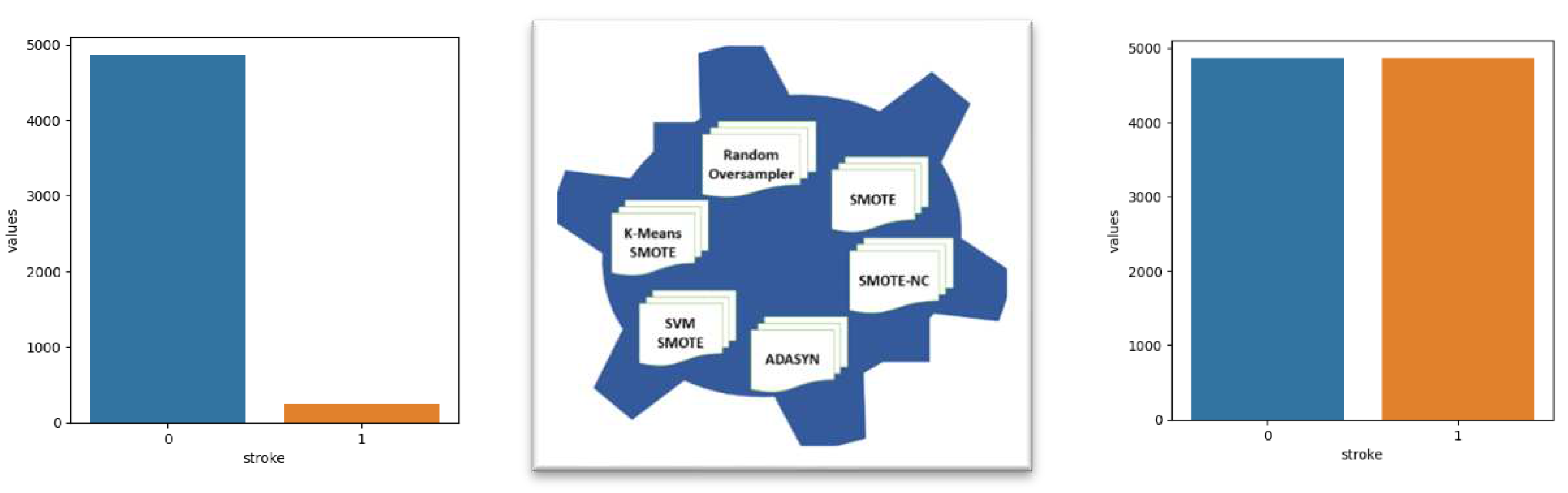
Figure 2.
Research Flowchart.
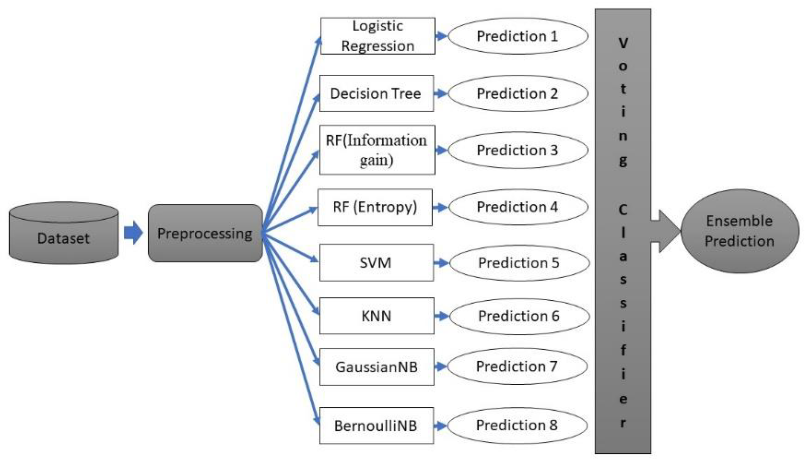
Figure 3.
Baseline (Without any Sampling).
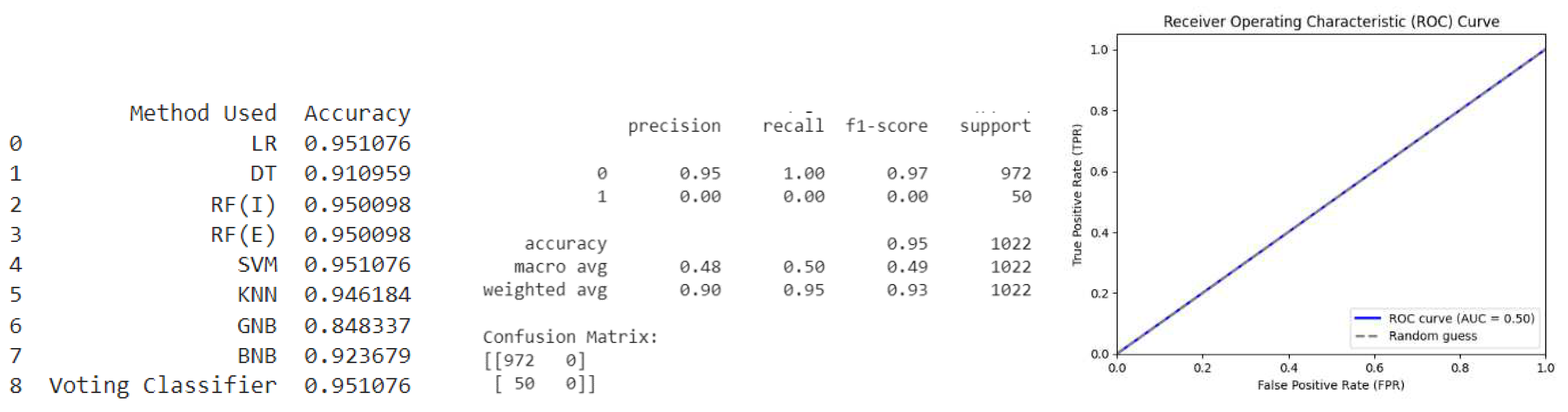
Figure 4.
Oversample (ROS).
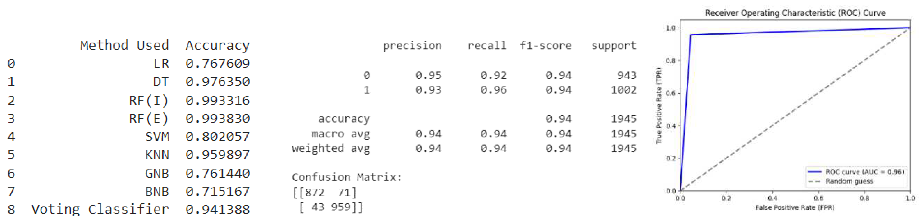
Figure 5.
Oversample (SMOTE).
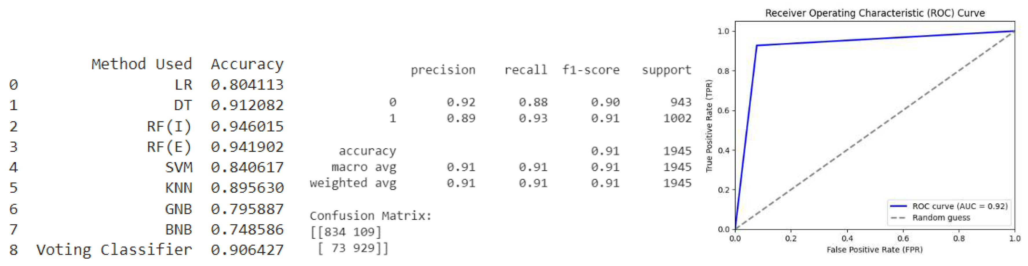
Figure 6.
Oversample (SMOTENC).
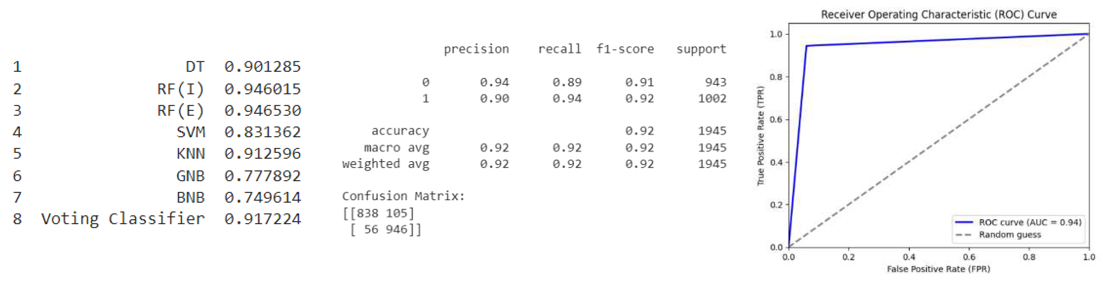
Figure 7.
Oversample (ADASYN).
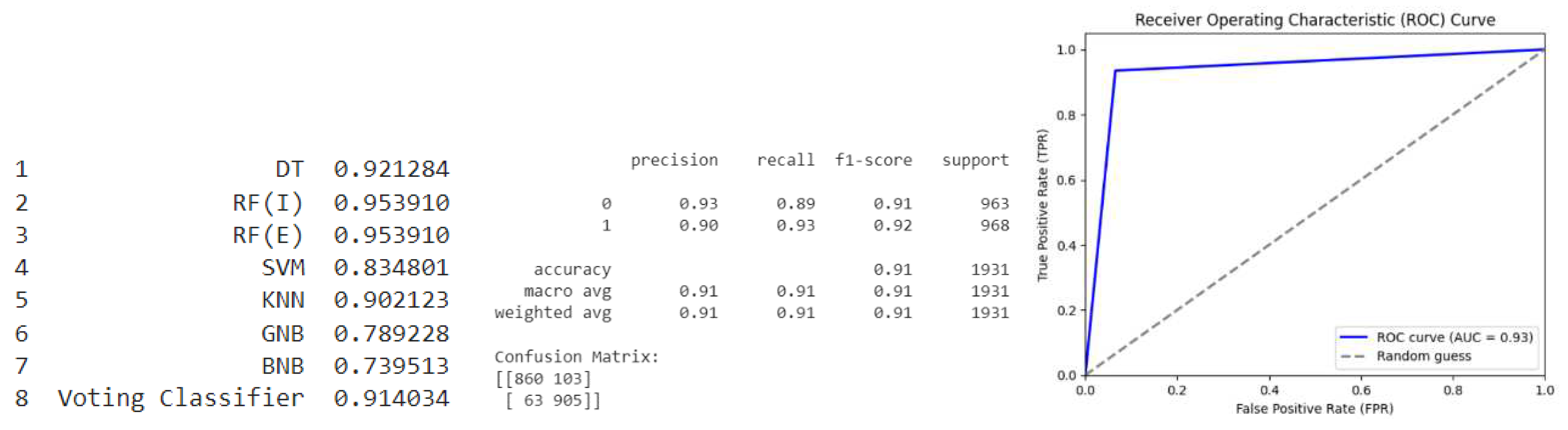
Figure 8.
Oversample (SVM SMOTE).
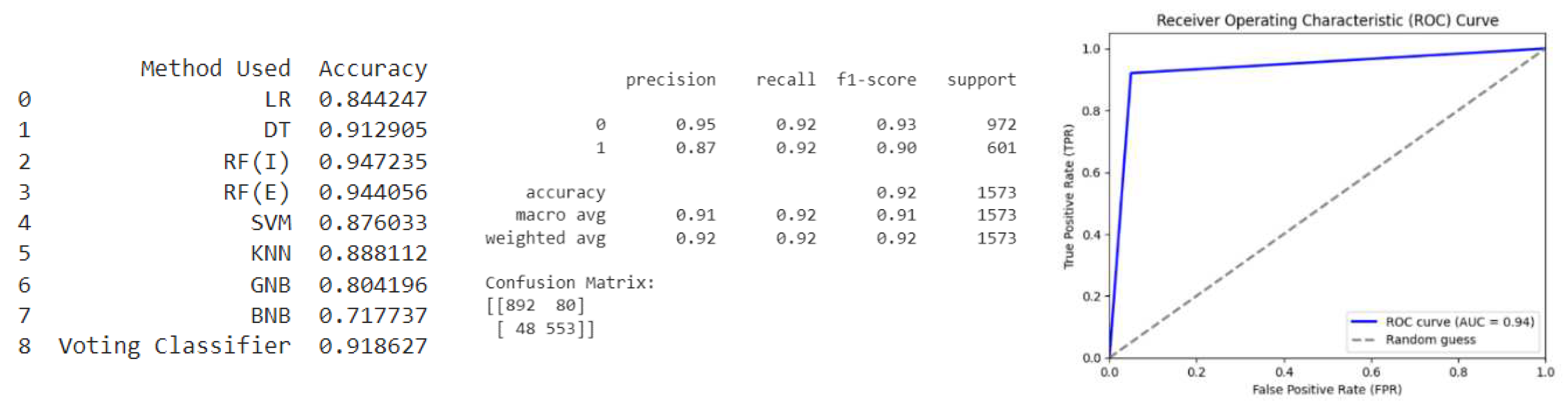
Figure 9.
Oversample (K Means SMOTE).
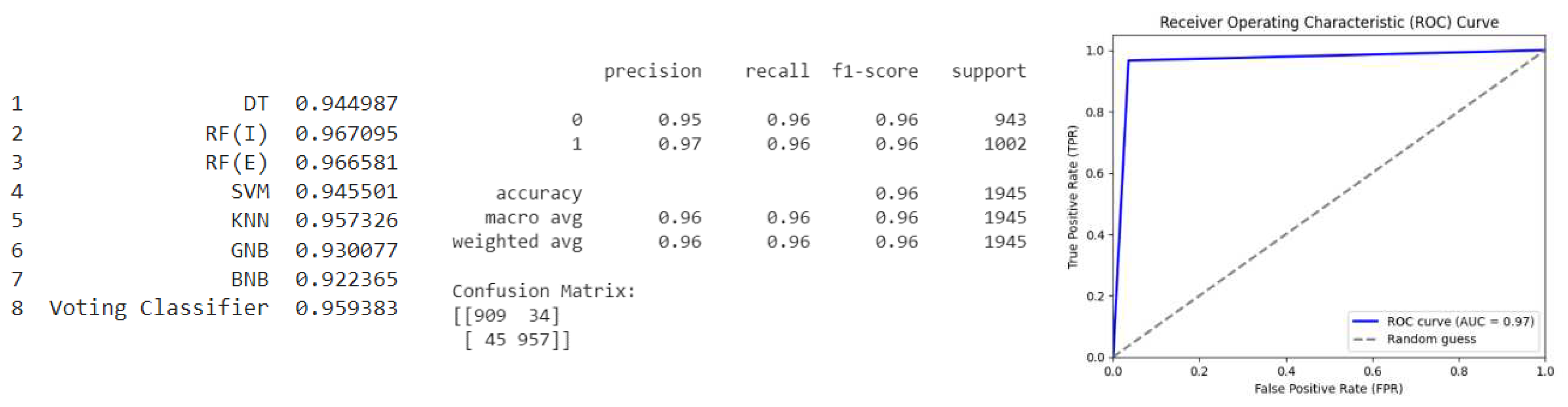

Table 1.
Comparison of Performance Metrics.
| Oversampling Techniques | Accuracy | False Positive | False Negative | ROC |
| Baseline | 95 | 0 | 50 | 0.5 |
| ROS | 94 | 72 | 43 | 0.96 |
| SMOTE | 91 | 109 | 73 | 0.92 |
| SMOTENC | 92 | 105 | 56 | 0.94 |
| ADASYN | 91 | 103 | 63 | 0.93 |
| SVM SMOTE | 92 | 80 | 48 | 0.94 |
| K Means SMOTE | 96 | 34 | 45 | 0.97 |
Disclaimer/Publisher’s Note: The statements, opinions and data contained in all publications are solely those of the individual author(s) and contributor(s) and not of MDPI and/or the editor(s). MDPI and/or the editor(s) disclaim responsibility for any injury to people or property resulting from any ideas, methods, instructions or products referred to in the content. |
© 2023 by the authors. Licensee MDPI, Basel, Switzerland. This article is an open access article distributed under the terms and conditions of the Creative Commons Attribution (CC BY) license (http://creativecommons.org/licenses/by/4.0/).
Copyright: This open access article is published under a Creative Commons CC BY 4.0 license, which permit the free download, distribution, and reuse, provided that the author and preprint are cited in any reuse.


