Diagnosing Alzheimer's Disease Levels Using Machine Learning and MRI: A Novel Approach

Alzheimer's disease is a neurological illness that worsens gradually. It is known as the most frequent cause of dementia. Moreover, Alzheimer's disease is a general term for memory loss and other cognitive impairments severe enough to disrupt daily life. The disease often grows in middle-aged and elderly people with the gradual loss of cognitive ability. Since the diagnosis of the illness is time consuming, a novel machine learning approach is proposed in this research to diagnose Alzheimer's levels based on Magnetic Resonance Imaging (MRI). More specifically, to provide distinct information for classification we have implemented the proposed method on a native MRI scans dataset containing three MRI channels; namely T1, T2, and, T2 tirm, which are shown in red, blue and green, respectively. The five middle layers of these three types of MRI scans are combined to form five RGB layers. In addition, we use a Convolutional Neural Network to classify each composed layer, and the final disease type is predicted using majority voting. finally, the F1-Score has been used to assess method performance, indicated that 92% of predictions of the proposed model were accurate.

Keywords:

Subject: Public Health and Healthcare - Public Health and Health Services

Introduction

Alzheimer’s disease (AD) is a degenerative neurological disease that primarily affects the elderly. The illness is frequently accompanied by a decline in cognitive abilities, such as daily tasks and decision-making skills, as well as a deterioration in social life abilities, such as mobility impairment, aphasia, and agnosia. Alzheimer’s disease has surpassed cancer as the most feared disease in the United States, killing more people than breast and prostate cancer combined [1]. Since symptomatic treatment is still only effective for a limited time, early diagnosis and prognosis of AD/MCI is critical. Therefore, many researchers devoted their efforts to developing an expert mechanism assisted by computers in predicting or diagnosis diseases. Recent research indicates MRI [2] and PET [3] can be sufficient means for classifying and diagnosis Alzheimer’s disease.

This disease’s progression can be divided into four following stages:

Healthy Control (HC)
Mild Demented
Moderate Demented
Alzheimer’s Disease

Throughout the last decade, efforts to identify Alzheimer’s biomarkers have accelerated. There is now broad consensus that the pathology of Alzheimer’s disease can be seen in brain scans years before the disease manifests itself [4].

Many researchers have adapted complex machine learning approaches to learn pathology patterns by classifying healthy controls from Alzheimer’s disease patients. Moreover, numerous studies have demonstrated the effectiveness of neuroimaging techniques in distinguishing Alzheimer’s disease patients from healthy controls [5].

The effectiveness of these algorithms (which have an accuracy rate of above 90%) has driven to attempts at fine-grained classification. including distinguishing healthy people from Mild Cognitively Impaired (MCI) individuals, and even determining which MCI subjects will develop Alzheimer’s disease [6,7].

Deep neural networks have emerged as one of the most powerful solutions for computer vision and medical imaging workloads in recent years. Although deep learning-based algorithms are adequate for a variety of medical tasks, they require large volumes of data, which is a significant barrier in medical applications such as neuroimaging and bioinformatics [8]. Furthermore, the lack of large datasets is widely recognized as the main distinction between medical imaging and other computer vision fields [5].

To gain a better understanding of the proposed method, it is vital to become acquainted with the three types of MRI scans T1, T2, and T2 tirm, as well as the differences of these three types of scans, which are explained below:

T1 weighted image:

Since T1-weighted volume scans with thin slices provide excellent anatomical detail, they have become a major component of scanning procedures for structural (or "morphological") imaging [9]. also, in the clinical perspective, T1-weighted are better at representing natural anatomy.

The longitudinal relaxation of a tissue’s net magnetization vector is used in a T1WI (NMV). A radiofrequency (RF) pulse, in essence, puts spins aligned in an external field (B0) into the transverse plane. They eventually return to B0’s initial equilibrium. The time it takes for a tissue’s protons’ spins to realign with the main magnetic field is reflected in its T1 (B0).

Fat quickly realigns its longitudinal magnetization with B0, appearing bright on a T1 weighted image. further, Water has much slower longitudinal magnetization realignment after an RF pulse resulting in less transverse magnetization. As a result, water appears dark and has low signal [11].

T2 weighted image:

T2-weighted images (T2WI) are one of the main pulse sequences on MRI scans and provide a map of proton energy within the body’s fatty AND water-based tissues. Fatty tissue is distinguished from water-based tissue by comparing with the T1 images – anything that is bright on the T2 images but dark on the T1 images is fluid-based tissue. For example, CSF1 is free fluid and contains no fat, so it appears white on the T2 images but dark on the T1. Moreover, it emits no signal on either T1 or T2 images because the bone cortex is black and contains no free protons [12].

Turbo Inversion Recovery Magnitude (TIRM):

The benefits of fat suppression in images include enhanced lesional contrast, as well as the elimination of fat-induced motion and chemical-shift misregistration artefacts [13].

Bone marrow pathology is evaluated by T2-weighted (T2-W), turbo spin-echo (TSE) MRI and short tau inversion recovery (STIR) imaging and, also shown these three types of imaging are highly effective [14-16]. However, Because of the long repetition times (TR), incorporation of inversion time (TI), and the spin echo (SE) component, traditional STIR sequences have extended scan periods of up to 12 minutes and more. Turbo inversion recovery magnitude (TIRM) images have similar quality and fat-suppression capabilities as STIR images [17, 18]. TIRM images can be acquired using low magnetic field systems and appear to be more stable than spectral fat suppression sequences (TSE with fat suppression) [13].

The proposed method has trained on a native dataset containing 300 MRI scans from various patients. As previously stated, the dataset instances have seventeen layers, and the five middle layers of each sample have been used to train and test the neural network. As a result, training the model on more data is made possible by using five middle layers of each sample.

Our method is built on a pipeline that includes novel data preprocessing, a classifier, and an ensemble learning component. Regarding data preprocessing a novel data preprocessing method has been used to convert scans to RGB images. The prepared data is fed into a convolutional neural network for Alzheimer’s variant diagnosis. Finally, we used majority voting to predict the best outcome which is shown the stage of the disease. Therefore, the proposed methodology can be summarized as follows:

A novel data preprocessing method is developed for efficient training on small datasets.
We have employed a convolutional neural network to classify the data which is provided by initial step.
majority voting is utilized to predict the final result.

The goal of this paper was to develop a novel method for detecting Alzheimer’s disease levels based on MRI scans. The proposed method contains three steps: a novel preprocessor, a CNN classifier, and ensemble learning. The approach can predict five levels of Alzheimer’s disease: healthy people, people with mild, medium, and severe cognitive impairments, and people with Alzheimer’s. The difference between this study and others is the incorporation of the intermediate layers of T1, T2, and T2 TIRM imaging to a single RGB image which contains valuable information.

Related Work

In this section, we mainly review the most relevant work. Firstly, the role of Machine learning in Alzheimer’s diagnosis is discussed since Machine learning approaches have been fruitful to diagnose the disease more accurately(Mahnaz Boush et al., 2023; M. Boush et al., 2023; Jafari et al., 2022; Kiaei et al., 2022, n.d.; Mohammadi et al., 2021; Safaei et al., 2023; Salari et al., 2023, 2022a, 2022a, 2022b, 2021). Then, we investigate several deep learning methods which are the most relevant to our research.

As one of the pioneering works by Haller [23] has used Support Vector Machines (SVMs) to classify stable MCI patients from progressive MCI ones with 98% accuracy. Although Support Vector Machines are effective for binary classification, they are insufficient for multi-class classification; hence, a deep learning-based classifier is used to classify the four Alzheimer’s disease variants in our work.

Deep learning approaches have grown over time and have been widely used in many applications. Due to the need for vast volumes of data for training a deep neural network, researchers and engineers initially utilized convolutional neural networks as a feature extractor [24]. In [paper reference number], Sarraf and et all have employed a convolutional neural network to classify Alzheimer’s patients from healthy cases. Sarraf has designed a CNN network similar to LeNet network [paper reference number] used to extract SIFT features from scans. Finally, they could classify test set cases with 96.85%. In 2015, Payan et al. proposed a method that has employed 3D convolution layers to process brain MRI scans. The network contains sparse AE and CNN. In this approach, the applied CNN layers have been already trained by sparse AE. Although this work has offered a novel approach to diagnosing Alzheimer’s disease, the results are not accurate enough [25].

Some works use more than one type of data to train their proposed approaches. For instance, functional Magnetic Resonance Imaging (fMRI) known as One of these types of data, is vastly used in medical diagnosis to measure the size of the initial visual cortex of a human and is widely utilized for brain topography detection. This scan type can demonstrate fruitful information about brain performance [26].

In [27], the authors have used a binary classifier to classify AD from HC. as the first step, they have employed a sufficient preprocessor for noise reduction. Since they have used two types of data to train the classifier, two pipelines have been utilized to feed data to the classifier. They used structural fMRI with a classification accuracy of 99.9% in one pipeline and structural MRI with a classification accuracy of 98.84 % in the other. Since the fMRI pipeline uses many 4D time-series images, the network training is time-consumed and it incurs a heavy computational burden.

Recently, researchers have been using transfer learning to overcome the lack of data. As stated previously, there is not enough data for training deep neural network models designed for medical diagnosis. Therefore, these models can benefit from transfer learning to diagnose more accurately. Farooq et al [28]. have used a preprocessing pipeline to convert MRI scans to gray matter. They have fed the prepared data to a CNN for classifying four classes (AD, MCI, LMCI, and, CN). The proposed approach benefits from transfer learning. Hence, it employs pre-train GoogleNet and ResNet which drive the network to predict more accurately. Hon et al. [29] classify healthy cases and Alzheimer’s patients using InceptionV4 and VGG16. They’ve also used image entropy to improve the training phase. YIGIT et al. [30] have employed a CNN to diagnose AD and MCI. MRI T1-Weighted scans have been used to diagnose AD and MCI. The authors have considered the image of skull stripping as a noise of scans and eliminated it during preprocessing. Additionally, the approach benefits from a CNN backbone which is responsible to extract feature maps from prepared scans. Finally, they have indicated that 80% of the approach predictions are accurate.

the stated methods are compared in Table 1. As illustrated in the table, most of the described papers use ADNI dataset collected in South America.

Methodology

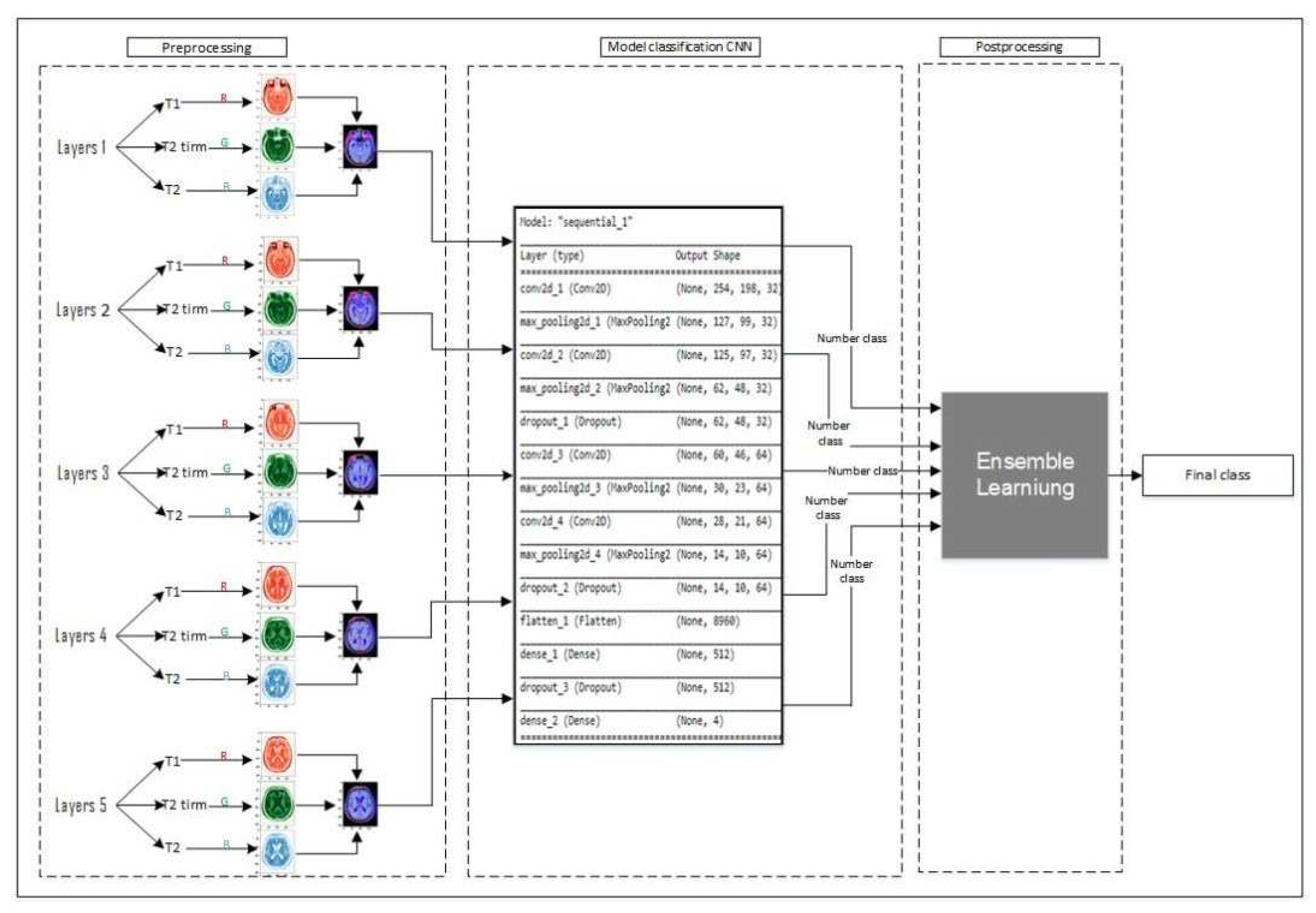
The proposed method classifies AD in two steps; i.e. Deep and ensemble learning. It consists of a novel data preprocessing method which makes our work unique. As shown in Figure 1, we choose five middle layers of each type of brain scan and integrate them to create an RGB image as shown in preprocessing section, then feed the provided layers to the CNN classifier and predict the type of each layer. finally, we use majority voting to predict the result. In section (section-num), we introduce the novel data preprocessing method. In section (section-num), we develop a convolutional neural network as a backbone for classifying the layers. Finally, we introduce the utilization of majority learning to predict the type of Alzheimer’s disease.

Preprocessing

TIV is commonly measured by T1-weighted MRI sequences, whereas T2-weighted MRI sequences provide superior contrast between the CSF bounding the premorbid brain space and surrounding dura mater [35]. Although integration of T1 and T2-weighted scans improve diagnostic ability in brain tissue [36], We employ TIV measurement based on T1, T2 and T2 TIRM to classification.

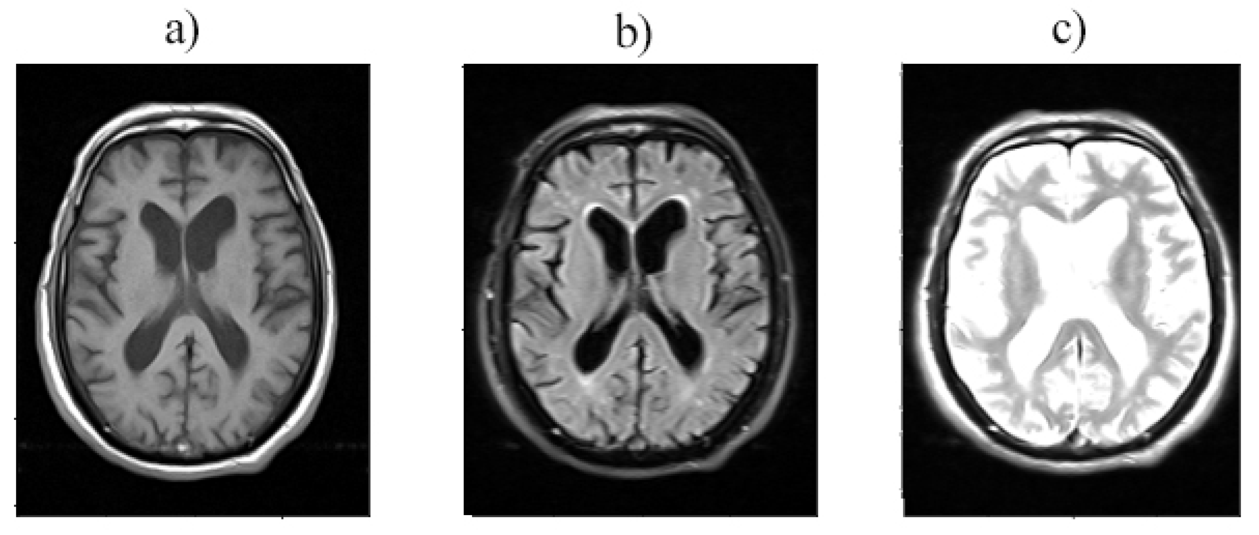
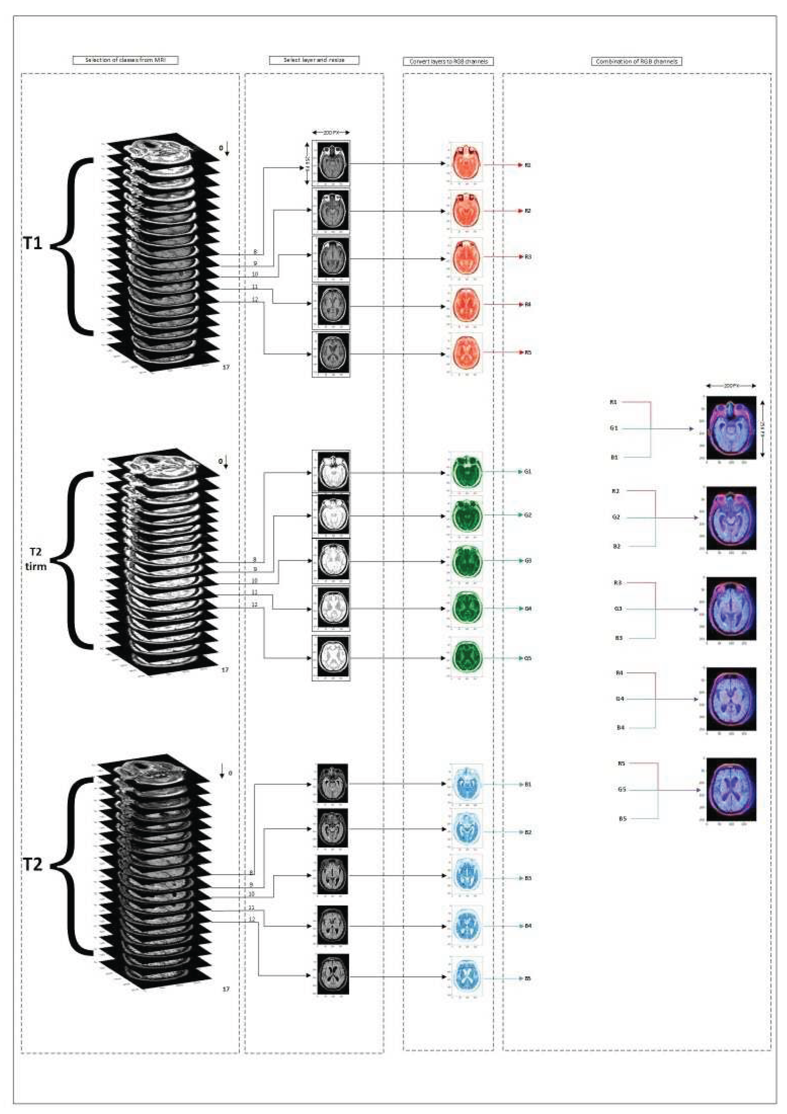
As illustrated in Figure 3, brain MRI scans contain seventeen 2D vectors, each representing a transverse view of different layer of the brain. the primary and final layers often provide us with less information about the disease. Hence, the five middle layers (layers 8-12) of scan types T1, T2, T2 TIRM have been employed in the data preprocessing step because the middle layers can be more effective in the classification portion.

Figure 2. Layer 12 is provided with a) T1, b) T2, and c) T2 TIRM imaging.

As depicted in Figure 3, each type of MRI imaging is regarded as an RGB channel. T1-weighted image, T2-weighted image, and T2 TIRM are referred to as the red, blue, and green channels, respectively. As shown in Figure 2, the integration of these three types of imaging provided extensive information for the classification step, Due to the differences in how the brain’s tissues and internal materials are displayed in each type of imaging.

Classification

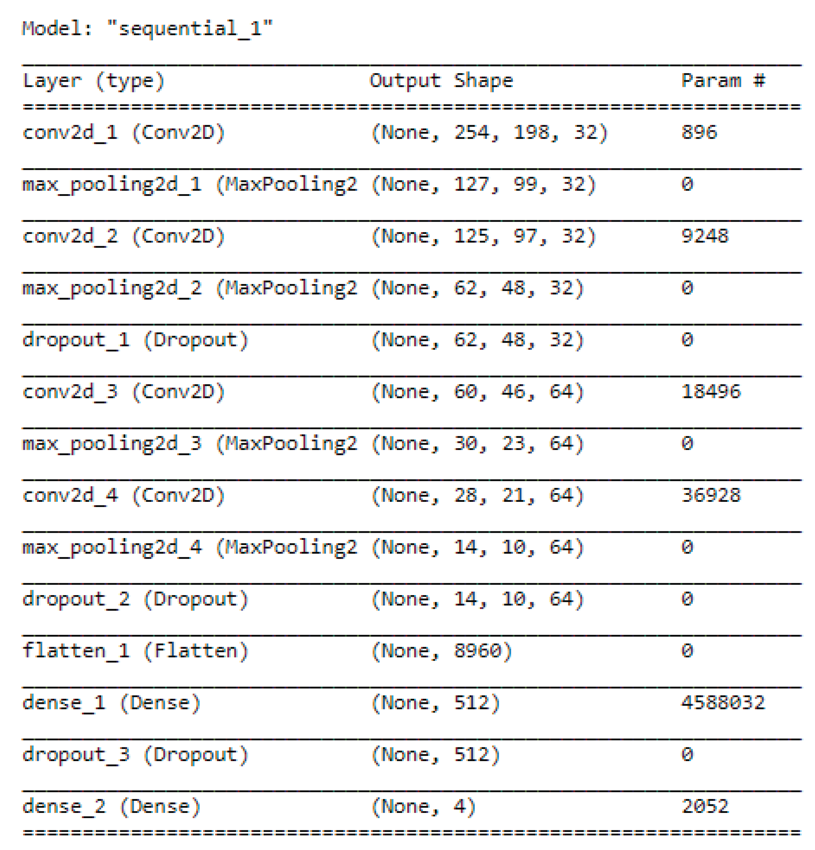
Here, we take the advantage of the Convolutional Neural Network to construct a backbone for visual feature extraction also use a fully connected neural network to classify extracted features from the provided layers produced during the data preprocessing step. In this research, we employ convolutional neural networks with fourteen layers to extract feature maps. As shown in Figure 4, the network contains four convolutional layers which are followed by a Max Pooling layer. Moreover, the architecture contains three Dropout, one Flatten, and two Fully Connected layers. Also, we use RELU as the activation function of hidden layers, and SoftMax has been employed in the fully connected layer.

Ensemble learning

Ensemble learning is a machine learning approach that involves training several learners to solve the same issue. Ensemble methods, in contrast to traditional machine learning approaches that attempt to learn a single hypothesis from training data, attempt to generate a set of hypotheses and aggregate them for usage.

Typically, an ensemble approach has constructed in two steps. First, several base learners are produced, which can be generated in a parallel fashion or in a sequential style where the generation of a base learner influences the generation of subsequent learners. Then, the base learners have integrated to use, where it employed majority voting for classification and weighted averaging for regression.

As previously stated, we employ a convolutional neural network to classify the five layers generated in step one. As a result, the classifier predicts five classes for each layer. The classifier predictions were then combined using majority voting (Also known as plurality voting) to determine the level of Alzheimer’s disease. Majority voting only use predicted labels to determine final result based on the most repetitions of a label. Therefore, during the test phase, five layers of different MRI images of the individual’s brain are given to the trained network and used majority voting to diagnose the level of disease progression.

One of the usages of such solutions at this stage is that the results can be significantly used by combining the same types of classifiers, each of which is presented in a different set of different training features. Different categories can be used in similar training sets.

The better performance of the same classifiers trained on the same set of features drives us to employ this solution to improve the classifier results. The used approach is significantly better than those taught by combining different classifiers but trained by similar feature sets [39]. As proven in [40], since the proposed model’s results are independent, majority learning improves performance in most cases. Hence, using more layers from MRI images will result in greater accuracy.

Dataset:

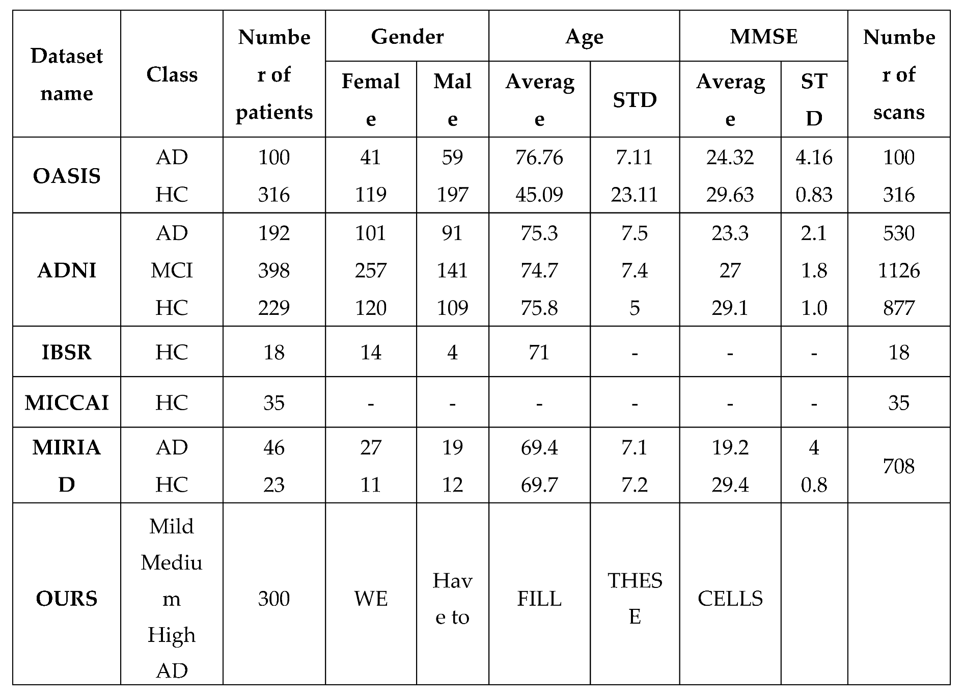
We use a native dataset collected by our research team. The dataset includes 300 samples gathered from 300 cases referred to a health center in Tehran. As previously stated, Each Sample consists of three different types of MRI imaging (T1-weighted, T2-weighted, and T2 TIRM). We use five layers of image types to train and test the proposed approach. During data preprocessing, we resize layers to 200 * 256 (height :200 and weight:256). Finally, 1500 training samples were generated by our novel preprocessing methodology. Furthermore, some publicly available datasets are used by researchers in their work. Table 1 compares our dataset to other publicly available datasets.

Table 2. Details of the OASIS, ADNI, IBSR, MICCAI and Ours datasets.

Experiments:

Implementation Details

The proposed approach is implemented in python with TensorFlow and Trained on one Nvidia GTX 1080 card. During the training process, the batch size is set as 32 and totally 50 iterations are performed by employing Adam with an initial learning rate 0.0001. In addition, we decrease the learning rate every 10 epochs. the testing phase uses the trained model to predict the class of each layer then executes the Majority voting algorithm for detaining the final result.

Metric

Many academics believe the accuracy metric which is known as the ratio between correct predictions and the total number of instances is the most realistic concept to measure the performance of an approach. In contrast, When the dataset is unbalanced, this metric loses its validity because it provides an over-optimistic estimate of the classifier’s ability on the majority class [52]. Hence, we use F1-Score to assess the performance of our approach because it retains its reliability even when using an unbalanced dataset.

The F-score, also known as the F-measure, is used to measure the performance of an approach. It consists of two main components: Precision and Recall, where Precision is the number of True Positive predicted results divided by the total number of Positive results, including those that incorrectly identified, and Recall is the number of True Positive predicted results divided by the total number of samples that should have been identified as Positive [52]. Additionally, in diagnostic binary classification, Precision is known as a positive predictive value, and Recall is also known as Sensitivity [53]. The F1-score equation is illustrated in Equation 1:

f 1 s c o r e = 2 \times \frac{p r e c i s i o n \times r e c a l l}{p r e c i s i o n + r e c a l l}

Results:

We tested various sets of hyperparameters to determine the best one because the more important hyperparameters in the proposed method are the selection and number of MRI imaging layers.

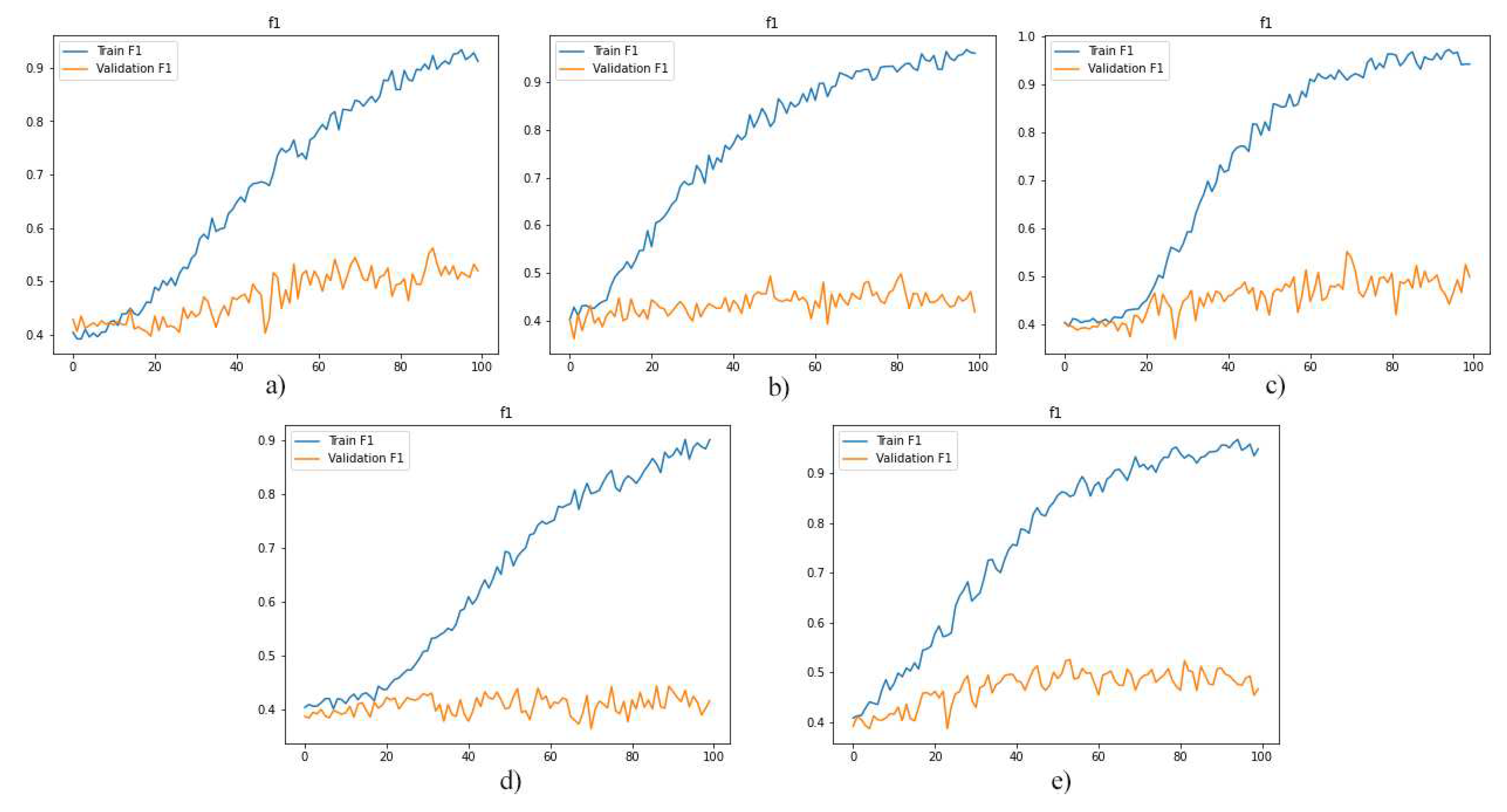
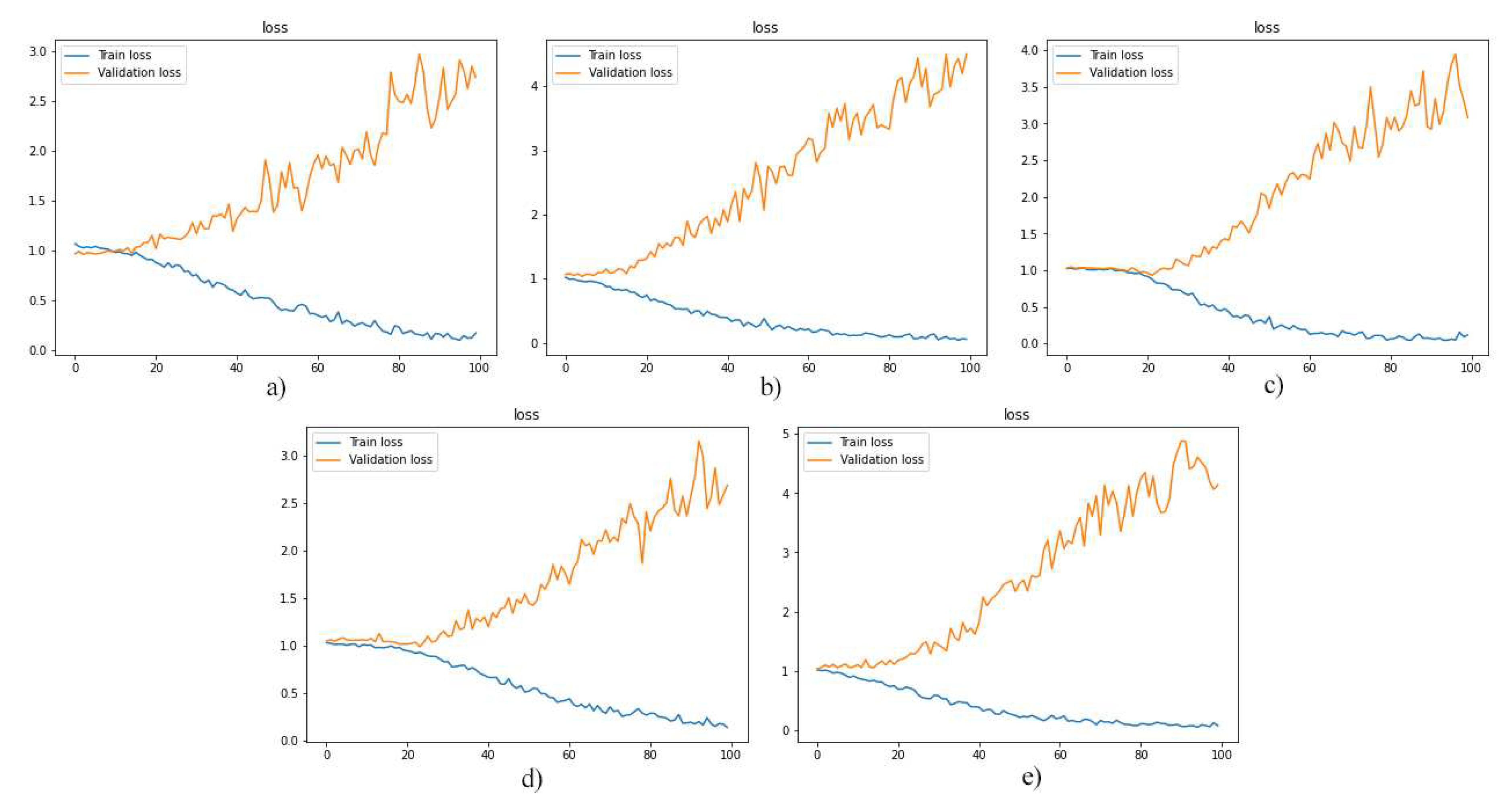
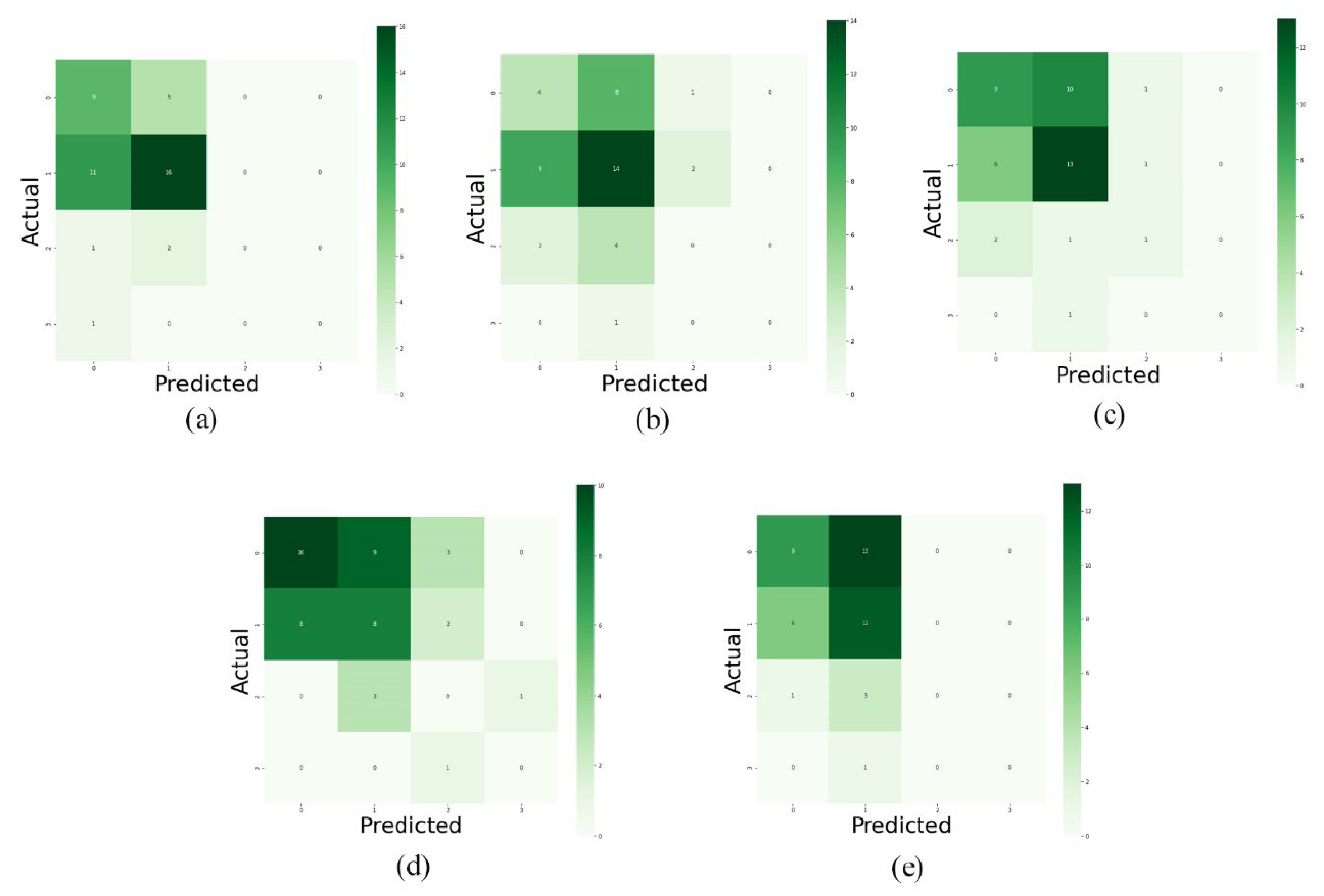
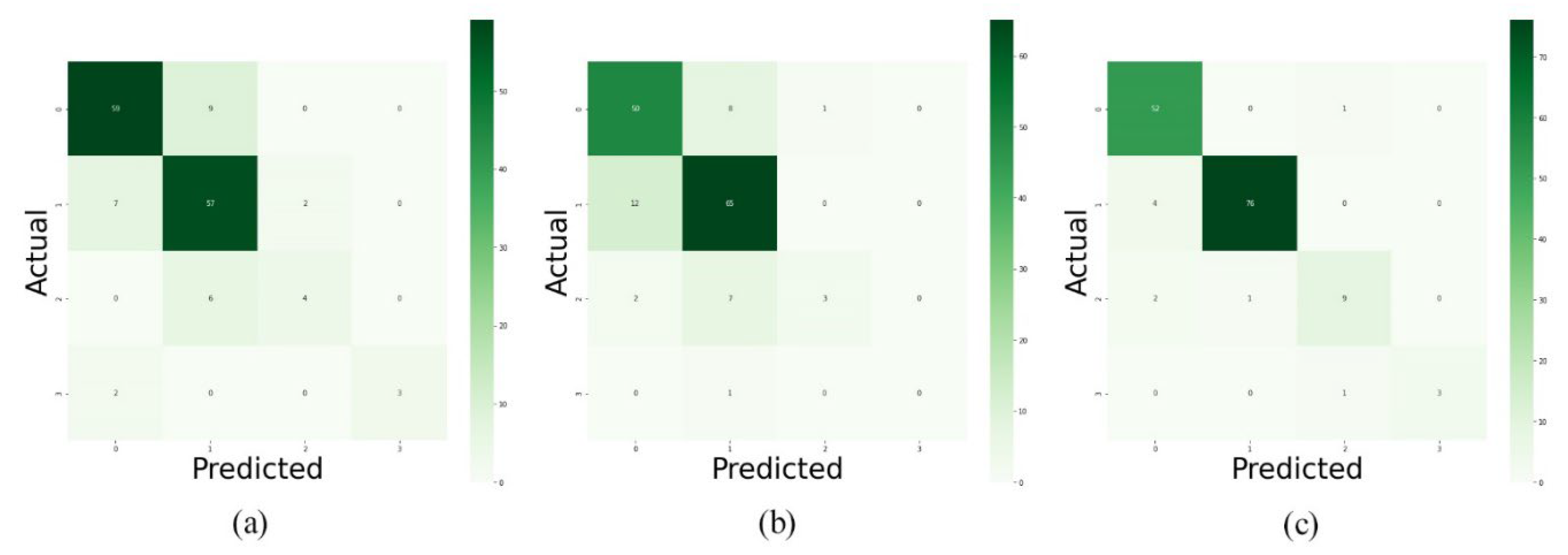
As a first experiment, we separately used the layers of MRI images for training the model. And, then we evaluated the performance of the trained models. The F1-score, model loss diagrams, and confusion matrix of the employment of layers 8, 9, 10, 11, and 12 are shown in Figure 5, 6, and 7, respectively. As shown in these figures (Figure 5, Figure 6 and Figure 7), this method of data utilization could not drive the model to have satisfactory and accurate performance on test data. Additionally, the model has overfitted due to the small amount of data. Therefore, we have used the integration of layers to prevent overfitting and be more precise predictions.

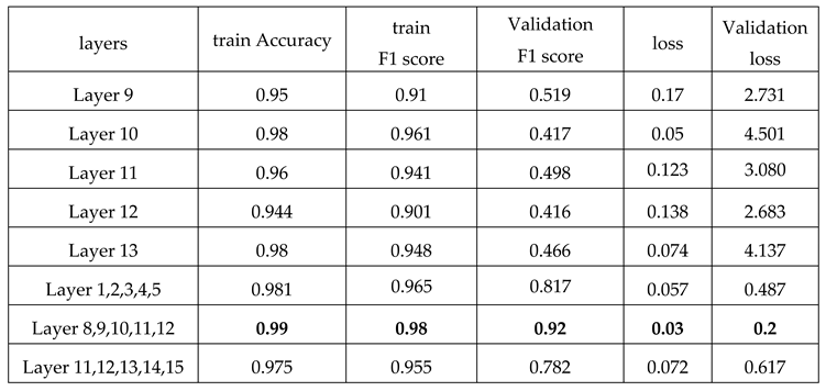
Since the approach has performed better when it is trained by integration of layers, we have trained the model with layers 1, 2, 3, 4, and 5 as well as layers 11, 12, 13, 14, and 15. As reported in Figure 8, Figure 9 and Figure 10 and Table 3, the best performance is provided by using layers 8 to 12. And it indicated that 92% of predictions of the proposed model were accurate.

Conclusions:

In this paper, we have introduced a three-step approach to predict the levels of Alzheimer’s progression using brain MRI scans. As the first experiment, we have trained the proposed model by T1-weighted, T2-weighted, and T2 TIRM images separately. And the results were not satisfactory. Hence, we used a hybrid method to integrate the five middle layers of T1 weighted, T2 weighted, and T2 TIRM imaging, treating each type of scans as an RGB channel to produce a single image with three RGB channels. Additionally, we have used mentioned method as data augmentation means to increase the amount of data in the dataset. As the next step, a convolutional neural network has been employed as a classifier to predict the type of each entry. In the last step, we have used majority voting to diagnose the levels of Alzheimer’s progression. As shown in Table 2, the F1-Score has been used to assess method performance, and it indicated that 92% of predictions of the proposed model were accurate.

Notes

1	Cerebro Spinal Fluid.

References

Alzheimer's Disease International (ADI). Available from: https://www.alzint.org/about/dementia-facts-figures/dementia-statistics/.
Cuingnet, R., et al., Automatic classification of patients with Alzheimer's disease from structural MRI: a comparison of ten methods using the ADNI database. neuroimage, 2011. 56(2): p. 766-781.
Nordberg, A., et al., The use of PET in Alzheimer disease. Nature Reviews Neurology, 2010. 6(2): p. 78-87.
C Vickers, J., et al., Defining the earliest pathological changes of Alzheimer’s disease. Current Alzheimer Research, 2016. 13(3): p. 281-287.
Ithapu, V.K., V. Singh, and S.C. Johnson, Randomized Deep Learning Methods for Clinical Trial Enrichment and Design in Alzheimer's Disease, in Deep Learning for Medical Image Analysis. 2017, Elsevier. p. 341-378.
Chincarini, A., et al., Integrating longitudinal information in hippocampal volume measurements for the early detection of Alzheimer's disease. NeuroImage, 2016. 125: p. 834-847.
Tangaro, S., et al., A fuzzy-based system reveals Alzheimer’s Disease onset in subjects with Mild Cognitive Impairment. Physica Medica, 2017. 38: p. 36-44.
Bengio, Y., Learning deep architectures for AI. 2009: Now Publishers Inc.
Lemieux, L., et al., Fast, accurate, and reproducible automatic segmentation of the brain in T1-weighted volume MRI data. Magnetic Resonance in Medicine: An Official Journal of the International Society for Magnetic Resonance in Medicine, 1999. 42(1): p. 127-135.
Bitar, R., et al., MR pulse sequences: what every radiologist wants to know but is afraid to ask. Radiographics, 2006. 26(2): p. 513-537.
Jeremy Jones, B.Y., T1 weighted image. Radiopaedia.org, 2021.
FRCR, D.G.L.-J.B.M.M. 2017; Available from: https://www.radiologymasterclass.co.uk/tutorials/mri/t1_and_t2_images.
Hauer, M., et al., Comparison of turbo inversion recovery magnitude (TIRM) with T2-weighted turbo spin-echo and T1-weighted spin-echo MR imaging in the early diagnosis of acute osteomyelitis in children. Pediatric radiology, 1998. 28(11): p. 846-850.
Arndt 3rd, W., et al., MR diagnosis of bone contusions of the knee: comparison of coronal T2-weighted fast spin-echo with fat saturation and fast spin-echo STIR images with conventional STIR images. AJR. American journal of roentgenology, 1996. 166(1): p. 119-124.
Golfieri, R., et al., The role of the STIR sequence in magnetic resonance imaging examination of bone tumours. The British journal of radiology, 1990. 63(748): p. 251-256.
Shuman, W., et al., Comparison of STIR and spin-echo MR imaging at 1.5 T in 45 suspected extremity tumors: lesion conspicuity and extent. Radiology, 1991. 179(1): p. 247-252.
Constable, R.T., R.C. Smith, and J.C. Gore, Signal-to-noise and contrast in fast spin echo (FSE) and inversion recovery FSE imaging. J Comput Assist Tomogr, 1992. 16(1): p. 41-47.
Panush, D., et al., Inversion-recovery fast spin-echo MR imaging: efficacy in the evaluation of head and neck lesions. Radiology, 1993. 187(2): p. 421-426.
Uhl, M., et al., Neuere Entwicklungen und Anwendungen in der MR-Sequenztechnik. Teil 1: Turbo-Spin-Echo, HASTE, Turbo-Inversion-Recovery, Turbo-Gradienten-Echo, Turbo-Gradienten-Spin-Echo-Sequenzen. Aktuelle Radiologie, 1998. 8(1): p. 4-10.
LeCun, Y., et al., Backpropagation applied to handwritten zip code recognition. Neural computation, 1989. 1(4): p. 541-551.
Deng, J., et al. Imagenet: A large-scale hierarchical image database. in 2009 IEEE conference on computer vision and pattern recognition. 2009. Ieee.
Krizhevsky, A., I. Sutskever, and G.E. Hinton, Imagenet classification with deep convolutional neural networks. Advances in neural information processing systems, 2012. 25: p. 1097-1105.
Haller, S., et al., Individual prediction of cognitive decline in mild cognitive impairment using support vector machine-based analysis of diffusion tensor imaging data. Journal of Alzheimer's disease, 2010. 22(1): p. 315-327.
Sarraf, S. and G. Tofighi, Classification of alzheimer's disease using fmri data and deep learning convolutional neural networks. arXiv preprint arXiv:1603.08631, 2016.
Payan, A. and G. Montana, Predicting Alzheimer's disease: a neuroimaging study with 3D convolutional neural networks. arXiv preprint arXiv:1502.02506, 2015.
Al-Shoukry, S., T.H. Rassem, and N.M. Makbol, Alzheimer’s diseases detection by using deep learning algorithms: a mini-review. IEEE Access, 2020. 8: p. 77131-77141.
Sarraf, S., G. Tofighi, and A.s.D.N. Initiative, DeepAD: Alzheimer’s disease classification via deep convolutional neural networks using MRI and fMRI. BioRxiv, 2016: p. 070441.
Farooq, A., et al. A deep CNN based multi-class classification of Alzheimer's disease using MRI. in 2017 IEEE International Conference on Imaging systems and techniques (IST). 2017. IEEE.
Hon, M. and N.M. Khan. Towards Alzheimer's disease classification through transfer learning. in 2017 IEEE International conference on bioinformatics and biomedicine (BIBM). 2017. IEEE.
YİĞİT, A. and Z. IŞIK, Applying deep learning models to structural MRI for stage prediction of Alzheimer's disease. Turkish Journal of Electrical Engineering & Computer Sciences, 2020. 28(1): p. 196-210.
Lei, B., et al., Predicting clinical scores for Alzheimer’s disease based on joint and deep learning. Expert Systems with Applications, 2022. 187: p. 115966.
Rutegård, M.K., et al., PET/MRI and PET/CT hybrid imaging of rectal cancer–description and initial observations from the RECTOPET (REctal Cancer trial on PET/MRI/CT) study. Cancer Imaging, 2019. 19(1): p. 1-9.
Yamanakkanavar, N., J.Y. Choi, and B. Lee, MRI segmentation and classification of human brain using deep learning for diagnosis of alzheimer’s disease: a survey. Sensors, 2020. 20(11): p. 3243.
Vuong, P., et al. Effects of T2-weighted MRI based cranial volume measurements on studies of the aging brain. in Medical Imaging 2013: Image Processing. 2013. International Society for Optics and Photonics.
Misaki, M., et al., Contrast enhancement by combining T 1-and T 2-weighted structural brain MR Images. Magnetic resonance in medicine, 2015. 74(6): p. 1609-1620.
Banja, J., AI Hype and Radiology: A Plea for Realism and Accuracy. Radiology: Artificial Intelligence, 2020. 2(4): p. e190223.
Werbin-Ofir, H., L. Dery, and E. Shmueli, Beyond majority: Label ranking ensembles based on voting rules. Expert Systems with Applications, 2019. 136: p. 50-61.
Delgado, J. and N. Ishii. Memory-based weighted majority prediction. in SIGIR Workshop Recomm. Syst. Citeseer. 1999. Citeseer.
Theodoridis, S. and K. Koutroumbas, Nonlinear classifiers. Pattern recognition, 2009: p. 151-260.
Hong, P., et al. Accuracy of classifier combining based on majority voting. in 2007 IEEE International Conference on Control and Automation. 2007. IEEE.
Marcus, D.S., et al., Open Access Series of Imaging Studies (OASIS): cross-sectional MRI data in young, middle aged, nondemented, and demented older adults. Journal of cognitive neuroscience, 2007. 19(9): p. 1498-1507.
Jack Jr, C.R., et al., The Alzheimer's disease neuroimaging initiative (ADNI): MRI methods. Journal of Magnetic Resonance Imaging: An Official Journal of the International Society for Magnetic Resonance in Medicine, 2008. 27(4): p. 685-691.
Landman, B.A. and S.K. Warfield, MICCAI 2012: Workshop on Multi-atlas Labeling. 2019: éditeur non identifié.
IBSR Dataset. [cited 4 June 2020; Available from: https://www.nitrc.org/projects/ibsr.
Malone, I.B., et al., MIRIAD—Public release of a multiple time point Alzheimer's MR imaging dataset. NeuroImage, 2013. 70: p. 33-36.
Wang, L., F. Chu, and W. Xie, Accurate cancer classification using expressions of very few genes. IEEE/ACM Transactions on computational biology and bioinformatics, 2007. 4(1): p. 40-53.
Sokolova, M., N. Japkowicz, and S. Szpakowicz. Beyond accuracy, F-score and ROC: a family of discriminant measures for performance evaluation. in Australasian joint conference on artificial intelligence. 2006. Springer.
Gu, Q., L. Zhu, and Z. Cai. Evaluation measures of the classification performance of imbalanced data sets. in International symposium on intelligence computation and applications. 2009. Springer.
Bekkar, M., H.K. Djemaa, and T.A. Alitouche, Evaluation measures for models assessment over imbalanced data sets. J Inf Eng Appl, 2013. 3(10).
Akosa, J. Predictive accuracy: A misleading performance measure for highly imbalanced data. in Proceedings of the SAS Global Forum. 2017.
Chicco, D. and G. Jurman, The advantages of the Matthews correlation coefficient (MCC) over F1 score and accuracy in binary classification evaluation. BMC genomics, 2020. 21(1): p. 1-13.
Buckland, M. and F. Gey, The relationship between recall and precision. Journal of the American society for information science, 1994. 45(1): p. 12-19.
Boush, M., Kiaei, A.A., Abadijou, S., Salari, N., Mohammadi, M., 2023. Drug combinations proposed by machine learning on genes/proteins to improve the efficacy of Tecovirimat in the treatment of Monkeypox: A Systematic Review and Network Meta-analysis.
Boush, Mahnaz, Kiaei, A.A., Safaei, D., Abadijou, S., Salari, N., Mohammadi, M., 2023. Recommending Drug Combinations using Reinforcement Learning to target Genes/proteins that cause Stroke: A comprehensive Systematic Review and Network Meta-analysis. https://doi.org/10.1101/2023.04.20.23288906.
Jafari, H., Shohaimi, S., Salari, N., Kiaei, A.A., Najafi, F., Khazaei, S., Niaparast, M., Abdollahi, A., Mohammadi, M., 2022. A full pipeline of diagnosis and prognosis the risk of chronic diseases using deep learning and Shapley values: The Ravansar county anthropometric cohort study. PLoS ONE 17, e0262701–e0262701. https://doi.org/10.1371/journal.pone.0262701.
Kiaei, A., Salari, N., Boush, M., Mansouri, K., Hosseinian-Far, A., Ghasemi, H., Mohammadi, M., 2022. Identification of suitable drug combinations for treating COVID-19 using a novel machine learning approach: The RAIN method. Life 12, 1456.
Kiaei, A.A., Boush, M., Abadijou, S., Momeni, S., Safaei, D., Bahadori, R., Salari, N., Mohammadi, M., n.d. Recommending Drug Combinations Using Reinforcement Learning targeting Genes/proteins associated with Heterozygous Familial Hypercholesterolemia: A comprehensive Systematic Review and Net-work Meta-analysis.
Mohammadi, M., Salari, N., Hosseinian Far, A., Kiaei, A., 2021. Executive protocol designed for new review study called: Systematic Review and Artificial Intelligence Network Meta-Analysis (RAIN) with the first application for COVID-19. Prospero.
Safaei, D., Kiaei, A.A., Boush, M., Abadijou, S., Salari, N., Mohammadi, M., 2023. Systematic review and network meta-analysis of drug combinations suggested by machine learning on genes and proteins, with the aim of improving the effectiveness of Ipilimumab in treating Melanoma.
Salari, N., Darvishi, N., Bartina, Y., Larti, M., Kiaei, A., Hemmati, M., Shohaimi, S., Mohammadi, M., 2021. Global prevalence of osteoporosis among the world older adults: a comprehensive systematic review and meta-analysis. Journal of Orthopaedic Surgery and Research 16, 669. https://doi.org/10.1186/s13018-021-02821-8.
Salari, N., Fatahi, B., Valipour, E., Kazeminia, M., Fatahian, R., Kiaei, A., Shohaimi, S., Mohammadi, M., 2022a. Global prevalence of Duchenne and Becker muscular dystrophy: a systematic review and meta-analysis. Journal of Orthopaedic Surgery and Research 17, 96. https://doi.org/10.1186/s13018-022-02996-8.
Salari, N., Hasheminezhad, R., Abdolmaleki, A., Kiaei, A., Razazian, N., Shohaimi, S., Mohammadi, M., 2023. The global prevalence of sexual dysfunction in women with multiple sclerosis: a systematic review and meta-analysis. Neurological Sciences 44, 59–66.
Salari, N., Hasheminezhad, R., Abdolmaleki, A., Kiaei, A., Shohaimi, S., Akbari, H., Nankali, A., Mohammadi, M., 2022b. The effects of smoking on female sexual dysfunction: a systematic review and meta-analysis. Archives of women’s mental health 1–7.

Figure 1. Illustration of the proposed approach.

Figure 3. T1, T2, and T2 TIRM have been used to create an RGB image.

Figure 4. Architecture of Convolutional Neural Network.

Figure 5. the diagrams illustrate the f1-score for models which were trained by layers: a)8, b)9, c)10, d)11 and e)12.

Figure 6. the loss diagrams of models which were trained by layers: a)8, b)9, c)10, d)11 and e)12.

Figure 7. Confusion matrix of predictions on validation data. Diagram (a) to (e) illustrate the confusion matrix of the models’ predictions which were trained by layers 8 to 12, respectively.

Figure 8. F1-Score diagrams a) the model is trained by layers 1, 2, 3, 4, 5 b) the model is trained by layers 11, 12, 13, 14, 15 c) the model is trained by layers 8, 9, 11, 12 (proposed layers for training the model).

Figure 9. the loss diagram of models which were trained by the various integration of layers. a) layers 1 to 5, b) layers 11 to 15, c) layers 8 to 12.

Figure 10. Confusion Matrix: a) layers 1 to 5 b) layers 11 to 15 c) layers 8 to 12.

Table 1. Comparing pioneer works.

Paper	Dataset	Accuracy
[25]	ADNI	AD vs. HC 95.39% (2D) 95.39% (3D) AD vs. MCI 82.24%(2D) 86.84% (3D) HC vs. MCI 90.13% (2D) 92.11%(3D)
[27]	ADNI	MRI adopted LeNet 98.79% MRI Adopted GoogleNet 98.8431% fMRI Adopted LeNet 99.9986% fMRI Adopted GoogleNet 100%
[24]	ADNI (binary classification)	CNN and LeNet-5 96.85%
[28]	ADNI	GoogleNet 98.88% ResNet-18 98.01% ResNet-152 98.14%
[29]	OASIS	VGG16 92.3% Inception V4 96.25%
[30]	OASIS (train) MIRAD (test)	Trained on all of 2 dimensional MRI 83%

Table 3. The table shows the accuracy, F1 score, and loss of models trained by various layers during train and test time.

Disclaimer/Publisher’s Note: The statements, opinions and data contained in all publications are solely those of the individual author(s) and contributor(s) and not of MDPI and/or the editor(s). MDPI and/or the editor(s) disclaim responsibility for any injury to people or property resulting from any ideas, methods, instructions or products referred to in the content.

© 2023 by the authors. Licensee MDPI, Basel, Switzerland. This article is an open access article distributed under the terms and conditions of the Creative Commons Attribution (CC BY) license (http://creativecommons.org/licenses/by/4.0/).

Copyright: This open access article is published under a Creative Commons CC BY 4.0 license, which permit the free download, distribution, and reuse, provided that the author and preprint are cited in any reuse.

MDPI Initiatives

Important Links

Choose an area of interest and we will send you notifications of new preprints at your preferred frequency.

Disclaimer