
Submitted:
14 June 2023
Posted:
14 June 2023
You are already at the latest version
Abstract
Diabetes becomes a life threatening non-communicable disease in the world, according to International Diabetic Federation (IDF) in 2023, an estimated 537 million adults (20-79 years) are living with diabetes, which is equivalent to 9.3% of the global adult population. This number is predicted to rise to 643 million by 2030 and 783 million by 2045. Over 3 in 4 adults with diabetes live in low- and middle-income countries. Diabetes is a persistent metabolic condition marked by increased levels of glucose in the bloodstream. It is a significant global health concern, affecting millions of individuals worldwide. It having the symptoms of drowsiness for the whole day if not properly examined or treated well. It is targeted to spread over the younger age community and the number is growing in the exponential fashion. Even day to day many advancements have come from the researcher to diagnose, to find solutions to prevent from newer entry. Authors have taken a dataset with 57 non diabetic and 20 diabetic patients with the total 28735 micro array gene to undergone pre-processing process and reduced up to 22960 gene data using Dimensionality Reduction (DR) such as Detrend Fluctuation Analysis (DFA), Chi square probability density function (Chi2PDF), Firefly algorithm Cuckoo search were used in this research. Meta heuristic algorithms like Particle swarm Optimization (PSO) and Harmonic Search (HS) are used for feature selection. Further seven classification techniques such as Non-Linear Regression (NLR), Linear Regression (LR), Logistics Regression (LoR), Gaussian Mixture Model (GMM), Bayesian Linear Discriminant Classifier (BLDC), Softmax Discriminant Classifier (SDC), Support Vector Machine – Radial Basis Function (SVM-RBF) are using to make a decision, predictive analysis and segregate the data according to the level of blood glucose as Diabetic Patient (DP) and Non-Diabetic Patient (NDP).
Keywords:
Type II Diabetes Mellitus
; Machine Learning
; Prediction
; Dimensionality Reduction
; Classifiers
1. Introduction
Statistics related to diabetes in worldwide: The global prevalence of diabetes among adults (20-79 years old) was 10.5% in 2021. Diabetes is more prevalent in low- and middle-income nations compared to high-income nations. The region with the highest prevalence of diabetes is the Middle East and North Africa, where 13.9% of adults have diabetes. Mortality: Diabetes was the ninth leading cause of death worldwide in 2019, with 4.2 million deaths attributed to the disease or its complications. Diabetes increases the risk of cardiovascular disease, and about 70% of people with diabetes die from cardiovascular disease. Complications: Diabetes can cause a range of complications, including neuropathy, retinopathy, nephropathy, and foot ulcers. Around 50% of individuals with diabetes remain undiagnosed, which means they may not be receiving appropriate treatment to prevent or manage these complications. Economic burden: The estimated global health expenditure on diabetes was $760 billion in 2019. Diabetes is a major cause of lost productivity, as it can lead to disability and premature death. The economic burden of diabetes is expected to rice in the future, as more people are diagnosed with the disease. These statistics highlight the growing global burden of diabetes and the urgent need for effective prevention and management strategies. Causes of the diabetic in most of the cases might be because of consuming food at irregular intervals, by not doing any physical activity and so on. A healthy human consumes a normal meal during the day, it increases the level of blood glucose around 120-140 mg/dL. Then release of insulin for equalize this increase of glucose level is pancreas primary duty. If it fails to release the sufficient amount of insulin from pancreas to equate the blood glucose level it called to be diabetic. The reason for insufficient amount of insulin secretion will be discussed later in challenges section.
India has a high prevalence of diabetes, which is also called as worlds capital in Diabetic. According to the International Diabetes Federation, in 2021, India had an estimated 87 million adults aged between 20-79 years with diabetes. This number is projected to increase to 151 million by 2045. The prevalence of diabetes in India varies across regions, with the southern and northern states having higher prevalence rates compared to the eastern and north eastern states. The states with the highest prevalence rates are Kerala, Tamil Nadu, and Punjab. Type 2 diabetes accounts for more than 90% of all cases of diabetes in India. Type 1 diabetes is less common and accounts for less than 10% of all diabetes cases. The complications of diabetes, such as heart disease, kidney disease, and eye disease, are also a significant problem in India. The burden of diabetes and its complications is significant in India and highlights the need for effective prevention and management programs.
In the medical field, classification strategies are broadly used to classify data into different classes according to some constraints. This is in contrast to using an individual classifier, which may not be as effective. Diabetes is a chronic illness that affects the body's ability to produce insulin, a hormone that regulates blood sugar levels [1]. As a result, people with diabetes often have high blood sugar levels, which can lead to a number of health complications. Certain indications of elevated blood sugar levels include heightened thirst, heightened appetite, and frequent urination.
1.1. Objectives:
The objective of this research is to develop a classification framework for analysing microarray gene data obtained from pancreases and accurately identifying individuals as either diabetic or non-diabetic. This objective will be achieved through the utilization of machine learning algorithms and metaheuristic algorithms.
Data Pre-processing and Dimensionality Reduction: Pre-process the microarray gene data from pancreases by handling missing values, normalizing the data, and addressing any data quality issues. Additionally, apply dimensionality reduction techniques such as DFA, Chi2PDF, Firefly search and Cuckoo search and it is divided into 2 categories of analyse the data such as classification of data without feature selection to 7 classifiers as NLR, LR, LoR, GMM, BLDC, SDC and SVM-RBF and then another category is with feature selection based on metaheuristic algorithm such as PSO and HS. These are to be enhance the performance of the classification models. These metaheuristic algorithms will be employed to optimize the selection of features, hyperparameter tuning, or model ensemble methods to achieve better classification accuracy. Conduct rigorous performance evaluation of the developed classification models and metaheuristic algorithms using appropriate metrics such as Accuracy (Acc), Precision (Prec), and F1-score (F1-S) Comparison with existing state-of-the-art methods will be performed to assess the effectiveness and superiority of the proposed approach.
Interpretability and Validation: Provide interpretability of the classification models to understand the most influential genes or features contributing to the identification of diabetic individuals. Validate the models using cross-validation techniques and assess their generalizability on unseen datasets to ensure reliable and robust performance. By accomplishing these objectives, the research aims to contribute to the field of medical diagnosis and provide a reliable and accurate method for classifying individuals as diabetic or non-diabetic based on microarray gene data from pancreases. The findings of this research can potentially enhance the understanding of the genetic factors associated with diabetes and pave the way for personalized treatment strategies and interventions for individuals at risk.
1.2. Challenges:
Identifying type II diabetic patients from microarray gene data obtained from the pancreas poses several challenges that need to be addressed.
Firstly, the high dimensionality of the gene data presents a significant challenge. Microarray experiments often generate a large number of genes, resulting in a high-dimensional feature space. This can lead to increased computational complexity and may require dimensionality reduction techniques to alleviate the curse of dimensionality.
Secondly, selecting informative features from the reduced dataset is crucial for accurate classification. Identifying the most relevant genes associated with type II diabetes is a non-trivial task, as the genetic basis of the disease is complex and involves various interactions. Optimization techniques, such as genetic algorithms or feature selection algorithms, need to be employed to identify the most discriminative features. Additionally, the heterogeneity of gene expression patterns within the pancreas and individual variations in gene regulation further complicate the classification task. The identification of robust and reliable classifiers that can effectively capture the subtle patterns in the data while generalizing well to unseen samples is another significant challenge.
1.3. Opportunities:
Early Detection and Intervention: The identification of non-diabetic individuals who are at a higher risk of developing type II diabetes can lead to early detection and intervention. By monitoring their gene expression patterns, lifestyle factors, and other relevant indicators, healthcare professionals can proactively provide personalized guidance, lifestyle modifications, and preventive measures to delay or even prevent the onset of diabetes. This can significantly improve the overall health outcomes and quality of life for at-risk individuals.
Personalized Treatment and Precision Medicine: Once individuals are accurately classified as diabetic or non-diabetic based on their gene expression profiles, the information can be used to develop personalized treatment strategies. This includes tailoring medication regimens, dietary recommendations, and exercise plans specific to the genetic profiles of diabetic patients. Moreover, this data can contribute to the emerging field of precision medicine, facilitating the development of targeted therapies that address the specific molecular mechanisms and pathways associated with type II diabetes.
Drug Development and Evaluation: The gene expression patterns obtained from the microarray data can provide valuable insights into the underlying biological processes involved in type II diabetes. This information can be utilized to identify potential drug targets and guide the development of novel therapeutic interventions. Additionally, the classified diabetic and non-diabetic groups can be leveraged to evaluate the effectiveness and safety of existing anti-diabetic drugs. This research can help identify subpopulations that may benefit more from specific medications, optimize dosage regimens, and enable the discovery of new treatment options.
2. Background
According to WHO [2], In India, 77 million people are living with type II diabetes, and 25 million are at high risk of developing it. Many people with diabetes are unaware of the severity of the condition, which can lead to serious complications such as nerve damage, reduced blood flow, and limb amputation. Shaw JE, Sicree RA, Zimmet PZ et al., [3] gave statistical data about the projection in the diabetic like, the global prevalence of diabetes is projected to increase from 6.4% in 2010 to 7.7% in 2030, affecting an estimated 439 million adults. This represents a significant increase in the number of people with diabetes, particularly in developing countries. Mohan V and Pradeepa R et al.,[4] proposed the prevalence of type 2 diabetes in India is increasing rapidly, and the country is expected to have the largest number of people with diabetes in the world by 2045. The high prevalence of diabetes in India is due to a combination of genetic, lifestyle, and demographic factors. The complications of type 2 diabetes, such as diabetic retinopathy, neuropathy, and cardiovascular disease, are a significant burden in India. There is a need for effective prevention and management strategies to address this issue. S. A. Abdulkareem et al.,[5] shared the experience by doing a comparative analysis of three soft computing techniques to predict diabetes risk: fuzzy analytical hierarchy processes (FAHP), support vector machine (SVM), and artificial neural networks (ANNs). The analysis involved 520 participants using a publicly available dataset, and the results show that these computational intelligence methods can reliably and effectively predict diabetes. The results indicate that the FAHP model is a highly effective method for diagnosing medical conditions that rely on multiple criteria, especially when the relative importance of each criterion is not clearly defined. The reported sensitivity values are 0.7312, 0.747, and 0.8793 for the FAHP, ANN, and SVM models, respectively.
Guillermo E. Umpierrez et al., [6] concluded the utilization of Continuous subcutaneous insulin infusion (CSII) and continuous glucose monitoring (CGM) systems are increasingly being used to manage diabetes in ambulatory patients. These technologies have been shown to improve glycemic control and reduce the risk of hypoglycemia. As the use of these devices increases, it is likely that more hospitalized patients will be using them. Health institutions should establish clear policies and protocols to allow patients to continue using their pumps and sensors safely. Randomized controlled trials are needed to determine whether CSII and CGM systems in hospitals lead to better clinical outcomes than intermittent monitoring and conventional insulin treatment. Aiswarya Mujumdar et al., [7] gave a study used various machine learning algorithms to predict diabetes. Logistic regression achieved the highest accuracy of 96%, followed by AdaBoost classifier with 98.8% accuracy.
K. Bhaskaran et al., [8] published in the journal Diabetes Care in 2016 found that a machine learning algorithm based on logistic regression was able to predict diabetes with an accuracy of 85%. A study published in the journal Nature Medicine in 2017 found that a machine learning algorithm based on decision trees was able to detect diabetes with an accuracy of 90%. A study published in the journal JAMA in 2018 found that a machine learning algorithm based on support vector machines was able to predict diabetes with an accuracy of 80%. Olta Llaha et al., [9] used the four classification methods mentioned above to classify data from a dataset of women with diabetes. The results of the study showed that the decision tree algorithm was the most accurate, with an accuracy of 79%. The Naive Bayes algorithm was the least accurate, with an accuracy of 65%. The SVM and logistic regression algorithms had accuracies of 73% and 74%, respectively. The authors of the article concluded that the decision tree algorithm is a promising tool for predicting diabetes. They also noted that the other three classification methods were also effective, but that the decision tree algorithm was slightly more accurate. The results of the study are promising, but it is important to note that the study was conducted on a dataset of women with diabetes. B. Shamreen Ahamed et al., [10] analysis the different classifiers were used in the study: The classification models utilized in the study encompassed Random Forest, Light Gradient Boosting Machine (LGBM), Gradient Boosting Machine, Support Vector Machine (SVM), Decision Tree, and XGBoost. The primary objective of the research was to enhance accuracy, with the LGBM Classifier achieving a notable 95.20% accuracy. Among the classifiers examined, the decision tree exhibited the highest accuracy of 73.82% without preprocessing. However, after preprocessing, the KNN classifier with k=1 and Random Forest achieved a perfect accuracy rate of 100%.
Neha Prerna Tigga et al., [11] explained six machine learning classification methods which includes, Logistic regression, Naive Bayes, Decision tree, Support vector machine, Random Forest, K-nearest neighbors were implemented to predict the risk of type 2 diabetes. Random forest had the highest accuracy of 94.10%. The parameters with the highest significance for predicting diabetes were age, family history of diabetes, physical activity, regular medication, and gestation diabetes. Maniruzzaman, Md, et al., [12] concluded in this study, a Gaussian process (GP)-based classification technique was used to predict diabetes. Compared the performance of four machine learning methods on a classification task. The methods are Gaussian Process (GP), Linear Discriminant Analysis (LDA), Quadratic Discriminant Analysis (QDA), and Naive Bayes (NB). The table shows that GP had the highest accuracy (81.97%), followed by LDA (75.39%), QDA (74.38%), and NB (73.17%). GP also had the highest sensitivity (91.79%) and positive predictive value (84.91%), while NB had the highest specificity (58.33%) and negative predictive value (51.43%).an accuracy of 81.97%, sensitivity of 91.79%, specificity of 63.33%, positive predictive value of 84.91%, and negative predictive value of 62.50%. These results were compared to other classification techniques, such as linear discriminant analysis (LDA), quadratic discriminant analysis (QDA), and Naive Bayes (NB). The GP model outperformed all other methods in terms of accuracy and sensitivity. Gupta, Sanjay Kumar, et al., [13] produced a result of study in India found that the Indian Diabetes Risk Score (IDRS) was 64% effective in identifying people with high risk of developing diabetes. The IDRS is a simple, cost-effective tool that can be used to screen large populations for diabetes. The study found that the IDRS was more effective in identifying people with high BMI (body mass index). People with a BMI of more than 30 were 6 times more likely to have a high IDRS than people with a BMI of less than 18.5. The study also found that the IDRS was more effective in identifying people with a family history of diabetes. People with a family history of diabetes were 3 times more likely to have a high IDRS than people without a family history of diabetes.
Howlader, Koushik Chandra, et al., [14] conducted a research study conducted on the Pima Indians, machine learning techniques were employed to identify significant features associated with Type 2 Diabetes (T2D). The top-performing classifiers included Generalized Boosted Regression modeling, Sparse Distance Weighted Discrimination, Generalized Additive Model using LOESS, and Boosted Generalized Additive Models. Among the identified features, glucose levels, body mass index, diabetes pedigree function, and age were found to be the most influential. The study revealed that Generalized Boosted Regression modeling achieved the highest accuracy of 90.91%, followed by impressive results in kappa statistics (78.77%) and specificity (85.19%). Sparse Distance Weighted Discrimination, Generalized Additive Model using LOESS, and Boosted Generalized Additive Models showcased exceptional sensitivity (100%), the highest area under the receiver operating characteristic curve (AUROC) of 95.26%, and the lowest logarithmic loss of 30.98%, respectively. Sisodia, Deepti et al., [15] did a study compared the performance of three machine learning algorithms for detecting diabetes: decision tree, support vector machine (SVM), and naive Bayes. The study used the Pima Indians Diabetes Database (PIDD) and evaluated the algorithms on various measures, including accuracy, precision, F-measure, and recall. The study found that naive Bayes had the highest accuracy (76.30%), followed by decision tree (74.67%) and SVM (72.00%). The results were verified using receiver operating characteristic (ROC) curves. The study's findings suggest that naive Bayes is a promising algorithm for detecting diabetes. Mathur, Prashant et al., [16] gave a study about Indian diabetic scenario, In India, 9.3% of adults have diabetes, and 24.5% have impaired fasting blood glucose. Of those with diabetes, only 45.8% are aware of their condition, 36.1% are on treatment, and 15.7% have it under control. This is lower than the awareness, treatment, and control rates in other countries. For example, in the United States, 75% of adults with diabetes are aware of their condition, 64% are on treatment, and 54% have it under control. Kazerouni, Faranak, et al., [17] explained the performance evaluation of various algorithms, the AUC, sensitivity, and specificity were considered, and the ROC curves were plotted. The KNN algorithm had a mean AUC of 91% with a standard deviation of 0.09, while the mean sensitivity and specificity were 96% and 85%, respectively. The SVM algorithm achieved a mean AUC of 95% with a standard deviation of 0.05 after stratified 10-fold cross-validation, along with a mean sensitivity and specificity of 95% and 86%. The ANN algorithm yielded a mean AUC of 93% with an SD of 0.03, and the mean sensitivity (Sens) and specificity (Spef) were 78% and 85%. Lastly, the logistic regression algorithm exhibited a mean AUC of 95% with an SD of 0.05, and the mean sensitivity and specificity were 92% and 85%. Comparative analysis of the ROC curves indicated that both Logistic Regression and SVM outperformed the other algorithms in terms of the area under the curve.
Figure 1.
Illustration of the work.
2.1. Role of Micro Array Gene
Microarray gene expression analysis plays a crucial role in understanding the molecular mechanisms and identifying gene expression patterns associated with various diseases, including diabetes. Here are some ways in which microarray gene expression analysis contributes to our understanding of diabetes: Identification of differentially expressed genes: Microarray analysis allows researchers to compare gene expression levels between healthy individuals and those with diabetes. By identifying differentially expressed genes, which are genes that show significant changes in expression between the two groups, researchers can gain insights into the molecular basis of diabetes. These genes may be directly involved in disease development, progression, or complications.
Uncovering disease subtypes and biomarkers: Microarray analysis can help identify distinct subtypes or phenotypes within a specific disease, such as different types of diabetes. By examining gene expression patterns across different patient groups, researchers can identify unique gene expression signatures associated with different disease subtypes. These subtype-specific gene expression patterns can potentially serve as diagnostic or prognostic biomarkers, enabling personalized treatment approaches. Pathway and functional analysis: Microarray gene expression data can be subjected to pathway and functional analysis to understand the biological processes and molecular pathways that are dysregulated in diabetes. By identifying the specific pathways and networks of genes involved, researchers can uncover the underlying mechanisms contributing to disease development and progression. Drug discovery and therapeutic targets: Microarray analysis can aid in the discovery of potential drug targets and therapeutic strategies for diabetes. By identifying genes that are dysregulated in the disease, researchers can pinpoint specific molecular targets that can be modulated with drugs or other interventions to restore normal gene expression patterns and mitigate the disease effects.
Personalized medicine and treatment response: Microarray analysis may help in predicting individual responses to certain treatments or interventions. By examining gene expression profiles in response to different therapies, researchers can identify molecular signatures that can guide personalized treatment decisions, leading to more targeted and effective interventions for individuals with diabetes.
Microarray genes play a significant role in the development and progression of diabetes. Microarrays are a type of gene expression profiling technology that can be used to measure the expression of thousands of genes simultaneously. This information can be used to identify genes that are differentially expressed in different conditions, such as disease states or in response to treatment.
In diabetes, microarrays have been used to identify genes that are involved in the following:
Insulin resistance: Insulin resistance is a condition in which the body's cells do not respond normally to insulin. This can lead to high blood sugar levels. Microarrays have been used to identify genes that are involved in insulin resistance.
Beta-cell dysfunction: Beta cells are the cells in the pancreas that produce insulin. In diabetes, beta cells can become damaged or destroyed. This can lead to a decrease in insulin production and an increase in blood sugar levels. Microarrays have been used to identify genes that are involved in beta-cell dysfunction.
Complications of diabetes: Diabetes can lead to a number of complications, including heart disease, stroke, kidney disease, blindness, and amputation. Microarrays have been used to identify genes that are involved in the development of these complications.
The information that is obtained from microarray studies can be used to develop new treatments for diabetes and its complications. For example, microarray studies have identified genes that are involved in insulin resistance and beta-cell dysfunction. This is used to develop new drugs that target these genes and improve the way that diabetes may be treated.
2.2. Organization of the paper
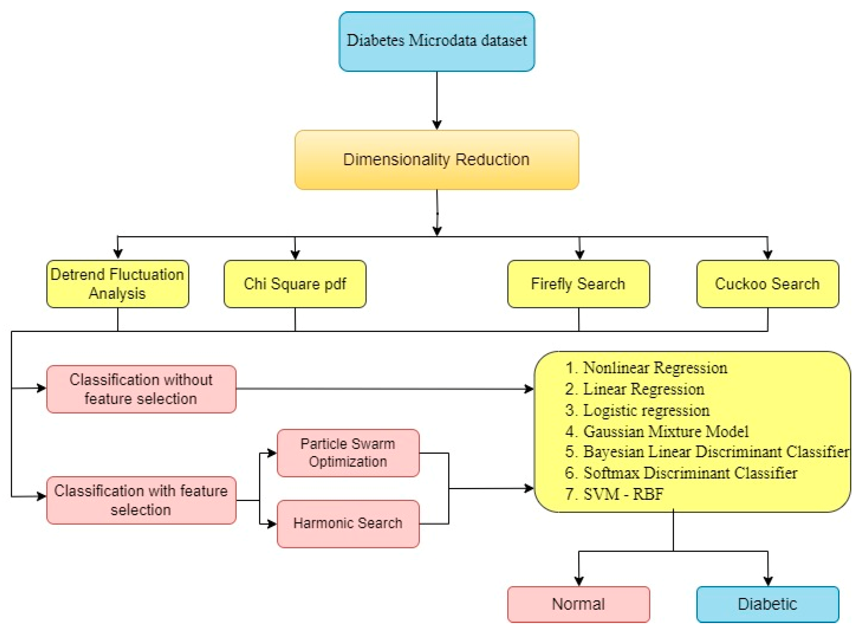
The research article is organized into seven chapters. Chapter 1 introduces the study and its objectives. Chapter 2 provides a background and literature review on diabetic and non-diabetic classes. Chapter 3 describes the dataset used, including the number of non-diabetic and diabetic classes. Chapter 4 explains the methods used to reduce the complexity of the dataset. Chapter 5 discusses the process of selecting relevant features using metaheuristic algorithms. Chapter 6 focuses on the classification stage, including the types of classifiers used and the evaluation metrics. Chapter 7 presents the results and provides a discussion on the findings. This organization ensures a clear and logical progression of the research, making it easier for readers to understand the study's structure and contributions.
3. Materials and Methods
Microarray gene data are readily available at many search engines, For the concern of pancreatic “Expression data from human pancreatic islets” were taken from Nordic islet transplantation programme for which these islets from cadaver donor of 57 Non-diabetic and 20 Diabetic of total 28735 gene data set arrived. (https://www.ncbi.nlm.nih.gov/bioproject/PRJNA178122). Preprocessing of data was performed for only 22960 genes per patients having the peak intensity with average valve were selected among the total samples. The logarithmic transformation was applied with a base 10 for standardized of individual samples with a value of 0 for mean and variance of 1.
3.1. Data set
Biological functions to detect the diabetic and its features of its secondary criteria in probability functions based on P values, a false positive error for selection of significant genes has also to be detected. The data available in many portals for human gene consists 28735 genes with 50 non-diabetic and 20 diabetic samples are considered for greatest minimal intensity across 70 samples. During dimensionality, reduction of both model and heuristic based, of diabetic and non-diabetic grouping as [2870*20] and [2870*50]. Further, it has been enhanced with feature selection based on 2 techniques named as Particle Swarm Optimization search and Harmonic Search, even more it was reduced by 287*20 and 287*50 with classifier techniques.
3.2. Need for Dimensionality Reduction
The need for dimensionality reduction techniques in the analysis of microarray gene data for type II diabetic class is crucial. Microarray experiments often generate a vast amount of gene expression data, resulting in a high-dimensional feature space. However, not all genes contribute equally to the classification task, and the presence of noise and irrelevant features can hinder the accuracy and interpretability of the results. Dimensionality reduction methods play a pivotal role in addressing these challenges by extracting the most informative features that are relevant to type II diabetes classification. These techniques aim to reduce the dimensionality of the data while preserving the discriminatory information, enabling efficient computation and improved performance of subsequent classification algorithms. By eliminating redundant and irrelevant features, dimensionality reduction can enhance the interpretability of the results, facilitate biological insights, and enable the identification of key genes and molecular pathways associated with type II diabetes. Overall, incorporating dimensionality reduction techniques into the analysis pipeline is essential for obtaining reliable and meaningful results from microarray gene data in type II diabetic class.
4. Dimensionality Reduction
The technique used to reduce the dimension of the matrix in the data set, first level of classification to be followed with the help of DFA, Chi2PDF, Firefly algorithm and Cuckoo search
4.1. Detrend Fluctuation Analysis (DFA)
To inspect the stationary and non-stationary functions of correlation, the short range and long-range relationship has used in DFA by Berthouze L et al, [18]. For typical application, the scaling of DFA is exponent to segregate the input data as rational and irrational. To estimate the functions of output class data it is useful to find the healthy and unhealthy objects as discriminate using DFA.
The algorithm is determined by the root mean square fluctuation of natural scaling and integrated time-series of input data in detrend.
(1)
Here X(i) is denoted as ith sample of input data
is specified as overall signal of mean value.
A(n) is indicated as estimated value in integrated time series.
(2)
Where bn(k) is predetermined window of scale n for a trend of kth point.
4.2. Chi Square Probability Density Function:
Among all the statics methods, a bit different approach of Chi square statistics methods Siswantining et al [19]. is the same according to fit test and the test of independence. Sample obtained from the data and it looks as referred as number of cases. It is to be represented as data is segregated in every incidence of occurrence in each group. In this statistics method of chi square, if the hypothesis is accurate, the expected number of cases in each category makes a statement of null hypothesis. The test based on the ratio of experimental data to the predicted values in each group. It is defined as,
(3)
Where, E_i refers to experimental data of cases in category i, and P_i refers to number of predicted values in category i, to compute the Chi square function is attained, the difference between the experimental data cases to the predicted value cases is calculated. Then the difference must be squared the values and get divided by the predicted value. Such that all the values in this category to be summed up for entire distribution curve to get the chi square statistics. For knowing the null hypothesis is a major concern, it depends on the data distribution. In Chi square, the alternative and null hypothesis is defined below,
Ho = Ei = Pi (4)
Ho = Ei≠ Pi (5)
If Ei – Pi is small for each type, then the expected value and predicted values are very close to each other, then the null hypothesis is real. When the expected data is not associate with predicted value of null hypothesis, then large difference is appeared between Ei – Pi. For real values of null hypothesis, small value of chi square statistics is arrived, if the value is false for null hypothesis the large value will attain. The degree of freedom is depending upon the variables of categories utilized to calculate the chi-square. In order to locate the required data, it is distributed according to the previously described distribution and the researcher asserts the use of chi-square statistics. By employing the chi-square distribution class, the researcher can conveniently access the chi-square distribution values. It is crucial for developers to take note of the degree of freedom as the sole parameter requiring optimization.
4.3. Firefly algorithm As Dimensionality Reduction
Yang, Xin-She (2010) [20] and Yang (2013) [21] was proposed a reliable metaheuristic model for real-life problem-solving techniques like scheduling of the events, classification of the system, dynamic problem optimization and economic load dispatch problems. The Fireflies algorithm works characteristic behaviour of the idealized flashing light of the firefly to attract the another one,
Three rules have identified in the firefly algorithm:
An attraction made to another fly regardless of the sex because of every fly was considered as unisex
“Opposite poles attract” like this the attractiveness is depends on the brighter side of one of the firefly is to another one which is slightly less bright. If none of the fly is getting brighter, it moves randomly in the surface.
If distance is increases, the brightness or light intensity of a firefly may decrease because the medium of air absorbs light in-between and thus the brightness of a firefly k which is seem by another fly firefly is given by:
(6)
Where β_k (0) represents the firefly (k) brightness at zero level, In the euclidean distance (if r=0), Light adsorption coefficient of the medium is represented by α, and Euclidean distance between i and k is denoted by r as
(7)
Where x_i and x_k are the firefly position of i and krespectively. If the brighter firefly is j, the its degree of attractiveness directs the movement of fly i, in which it is based on (Yang & He 2013)
(8)
Where refers to the random parameter and in general it was represented as, and it was expended as random number generator using uniform distribution where lies between the ranges of [-1, +1]. In-between representation in this equation contains the accountability of movement of firefly towards firefly . The last term in this above equation gives the movement of solution away from the optimum value in local when such as incident occurs.
4.4. Cuckoo Search algorithm as Dimensionality Reduction
Yang, X. S and Deb, S (2009) [22] proposed another metaheuristic model to give the finite solutions which is used for solving real- world problems such as Event scheduling, dynamic problem optimization, classifications and problems in economic load dispatch. Exciting breeding behaviours is the main objective of learning this algorithm and it’s particularly concentrates on the oblige brood parasitism of certain cuckoo birds. The characteristics of cuckoo species model based on the cuckoo search algorithm, which is exactly dumping the eggs in the inner portion of their nest of others birds and afterward it makes the host bird to cultivate their own hatchlings. Some exceptional cases also witnessed in this process have directly conflict with the intruded cuckoos. Main idealized thing in the cuckoo search algorithm is breeding characteristics and applicable for many real time optimization problems.
A simple solution obtained from each egg in a host nest, with continuation a new solution derived from own egg in cuckoo birds. The main aims to get the better solution (Cuckoos) to be replaced with the less best fit. Each egg has one solution, wherein as each nest has its multiple egg by finding the best one to signifies a set of solutions.
Three rules (Xin-She Yang & Suash Deb 2009) for Cuckoo search algorithm depends on:
- Cuckoo lays an egg at a time, and it kept inside a arbitrarily selected shell.
- To create a consecutive generation, the best host shell with good quality egg to transfer its own
- Fixed no of hosts nest is accessible, indeed cuckoo place an egg in a nest indeed with a probability of P_(a ) ϵ (0,1) ; where P_a Cuckoo egg probability. To construct a new nest in additional location, the host one can demolish the cuckoo egg’s away or it will be removing the nest.
Moreover, yang and deb predicted an appropriate result for searching techniques is based on random-walk (RW) and its performance is better than Lévy flights than RW. The conventional method is modified for the proposed method using classification techniques.
Lévy flights denotes the RM characteristics of birds position and its performance is to obtain the following position P_i^((t+1)) based on the present position P_i^((t)) mentioned in the article by Gandomi et al. (2013) [23]
(9)
Where ⊕ and β represents the starting point multiplication and step size. Commonly, β>0 , is interrelated to the depth of variation and its interest of problem consideration. For almost the classification problems, randomly fixed the values as 1. The above equation is based on the RW on stochastic model. To find out the following position is depending on present position and transition probability for RM which denotes on Markov chain. Gandomi et al. (2013) [23] discussed about the calculation of random length step and its comparison with the RM based on Lévy flight.
(10)
In the classification problem for fixing the value of β is tuned to 0.2, which denoted the infinite variance with infinite mean. Power law-based step length distribution approach by using a heavy tail for RW to principally followed cuckoo’s consecutive step. To speed up the classification process, the best solution is arrived using Lévy walk.
4.1. Statistical Analysis
The dimensionally reduced Micro array genes through four DR methods are analysed by the statistical parameters like mean, variance, skewness, kurtosis, Pearson correlation coefficient (PCC), and CCA to identify whether the outcomes are representing the underlying micro array genes properties in the reduced subspace. Table 2 shows the statistical features analysis for four types of Dimensionally Reduced Diabetic and Non-Diabetic Pancreas micro array genes. As shown in the Table 2 that in the DFA and Cuckoo search-based DR methods depicts higher values of mean, and variance among the classes. As in the Chi2 pdf and Firefly Algorithm display low and overlapping values of mean and variance among the classes. The negative skewness depicted only by the Chi2 pdf DR method which indicates the presence of skewed components embedded in the classes. Firefly algorithm indicates unusual flat kurtosis and Cuckoo Search DR method indicates negative kurtosis. This in turn leads to the observance that the DR methods are not modifying the underlying Micro array genes characteristics. PCC values indicate the high correlation with in the class of attained outputs. This subsequently exhibits that the statistical parameters are associated with non-Gaussian and non-linear one. The same is further examined by the histogram, Normal probability plots and Scatter plots of DR techniques outputs. Canonical correlation Analysis (CCA) visualizes the correlation of DR methods outcomes among the Diabetic and non-Diabetic cases. The low CCA value in the Table 1 indicates that the DR outcomes are less correlated among the two classes.
Figure 2 shows the Histogram of Detrend Fluctuation Analysis (DFA) Techniques in Diabetic Gene Class. It is noted in the Figure 2 that the histogram displays near quasi-Gaussian and presence of non-linearity in the DR method outputs
Figure 3 displays the Histogram of Detrend Fluctuation Analysis (DFA) Techniques in non-Diabetic Gene Class. It is observed from the Figure 3 that the histogram displays near Gaussian and presence of non-linearity and gaps by the DR method outputs.
Figure 4 exhibits the normal Probability plot for Chi Square DR Techniques Features for Diabetic Gene Class. As indicated from the Figure 4 that the normal probability plot displays the total cluster of Chi Square DR outputs and also the presence of non-linearly correlated variables among the classes.
Figure 5 depicts the normal Probability plot for Chi Square DR Techniques Features for non-Diabetic Gene Class. As shown from the Figure 5 that the normal probability plot displays the total cluster of Chi Square DR outputs and also the presence of non-linearly correlated variables among the classes. This is due to low variance and negatively skewed variables of the DR method outcomes.
Figure 6 indicates the normal Probability plot for Firefly Algorithm DR Techniques Features for Diabetic Gene Class. As mentioned by the Figure 6 that the normal probability plots display the discrete clusters for firefly DR outputs. This indicates the presence of non-Gaussian and non-linearly variables within the classes. This is due to low variance and flat Kurtosis variables of the DR method outcomes.
Figure 7 demonstrates the normal Probability plot for Firefly Algorithm DR Techniques Features for non-Diabetic Gene Class. As mentioned by the Figure 7 that the normal probability plots display the discrete clusters for firefly DR outputs. This indicates the presence of non-Gaussian and non-linear variables within the classes. This is due to low variance and flat Kurtosis variables of the DR method outcomes.
Figure 8 shows the Scatter plot for cuckoo search Algorithm DR Techniques Features for Diabetic and non-Diabetic Gene Class. As depicted by the Figure 8 that the scatter plots from Cuckoo search displays the total scattering of the variables of the both classes across the entire subspace. The scatter plot also indicates the presence of non-Gaussian, non-linear and higher values of all statistical parameters. Furthermore, the firefly and Cuckoo search algorithms will heavy computational cost on the classifier design in order to reduce the burden of the classifiers feature selection process utilizing Particle Swarm Optimization (PSO) and Harmonic search methods are initiated.
5. Feature selection
In the field of optimization, finding the optimal solution for complex problems is a significant challenge. Traditional optimization algorithms often struggle to handle high-dimensional search spaces or non-linear relationships between variables. To address these challenges, authors have identified two such popular metaheuristic algorithms among many, one is about the inspiration from natural and another one is from abstract concepts. Those two are Particle Swarm Optimization (PSO) and Harmonic Search (HS).
5.1. Particle Swarm Optimization (PSO)
Particle Swarm Optimization (PSO), Rajaguru H, et al., [24], one of the best and simple understanding among all search algorithm. It used some basic parameters for initial search and population called particles. In a h-dimensional space, the any of the particle will give best possible solution for processed and analysed. Every particle is need to be traced and positioned for the optimized values to achieve.
Position traced by:
Velocity traced by: The updated velocity of each particle is given by
(11)
Where are the random variable search in the ranges from 0 to 1. are the acceleration coefficient that check the movement (motion) of the particles.
(12)
Once a particle achieves its best position, it advances to the subsequent particle. The best position is denoted as "p-best" to represent the individual particle's optimal state, while "g-best" represents the best position among all particles,
The weight function is represented as
(13)
Steps for implementation:
Step1: Initialization for the process
Step2: For each particle the dimension a space is denoted as h
Step 3: Initialization the particle position as and velocity as Step 4: Evaluate the fitness function
Step 5: Initialize the with a copy of Step 6: Initialize the with a copy of with the best fitness function
Step 7: Repeat the steps until stopping criteria is satisfied
Stopping criteria:
(14)
(15)
5.2. Harmonic Search (HS)
Harmony search (HS) is a metaheuristic algorithm that draws inspiration from the evolution of music and the quest for achieving perfect harmony. Bharanidharan, N et al., [25] introduced HS as an algorithm that emulates the improvisational techniques employed by musicians. The HS algorithm involves a series of steps to be implemented,
Step 1: Initialization
The optimization problem is generally formulated as minimizing or maximizing the objective function f(x), subject to yi ∈ Y, where i = 1, 2, ..., N. In this formulation, y represents the set of decision variables, N denotes the number of decision variables, and Y represents the set of all possible values for each decision variable (i.e., yiLo ≤ yi ≤ yiUp, where yiLo and yiUp are the lower and upper bounds for each decision variable). Along with defining the problem, the subsequent step involves initializing the following parameters for the Harmonic Search (HS) algorithm.
Step 2: Memory Initialization
The Harmony Memory (HM) refers to a matrix that holds the collection of decision variables. In the context of the overall optimization problem, the initial HM is established by generating random values for each decision variable from a uniform distribution, which is confined within the bounds of yiLo and yiUp.
Step 3: New Harmony Development
During the process of solution improvisation, a new harmony is created by adhering to the following constraints:
- Memory consideration
- Pitch adjustment
- Random selection
Step 4: Harmony memory updation:
Compute the fitness function for both the previous and updated harmony vectors. If the fitness function of the new harmony vector is found to be lower than that of the old harmony vector, substitute the old harmony vector with the new one. Otherwise, retain the old harmony vector.
Step 5: Stopping criteria
Continue repeating Steps 3 and 4 until the maximum number of iterations is reached.
The effectiveness of the feature selection methods outputs is analysed through the significant of the p-value from t-test. Table 3 shows the p-value significant for the PSO and Harmonic Search feature selection methods outputs after four DR techniques. As tabulated in the Table 3 that the PSO Feature selection method not showing any significant p-values among the classes for the all four DR methods. As in the case of Harmonic Search Feature selection shows certain p-value significance for DFA and Firefly DR Techniques for the Diabetic class. At the same time all other DR methods exhibits non-significant p-values. This p-value will be measure to quantify the presence of outliers, non-linear and non-Gaussian variables among the classes after feature selection methods.
6. Classification Techniques
There are seven classification models used after dimensionality reduction 1. Non-linear regression, 2. Linear regression and 3. Logistic regression. 4. Gaussian Mixture Model 5. Bayesian Linear Discriminant classifier 6. Softmax Discriminant Classifier 7. Support Vector Machine – Radial Basis Function
6.1. Non-Linear regression:
The behaviour of the system, which denotes as mathematical expression for easy representation and analysis to get the accurate best-fit line in-between the classifier values. In this case author uses the mathematical way for the linear system of the variables like (a, b) for the equation in a linear mode, y=ax+b, but in case of non-linear, the values of variable a and b are nonlinear and random variable respectively. To get the least some of the squares is one of the primary objectives of non-linear regression. The values it measures from the dataset mean to be observed as number of samples it acquired. The difference between the mean and all the dataset point is to calculate using computing techniques for dataset mean value. Then take the difference values and squared each value and at last, it is added together for all the squared values. If the function gets better-fit values in the point of data set, it means the minimum value of sum of square values is obtained. Non-linear model requires more attention than linear model because of its complexity nature and researchers found many methods to reduce its complexity as levenberg-Marquard and Gauss-Newton Methods. The estimation parameters can be done for non-linear systems by using least square methods. To reduce the residual sum of squares the equation must be used for non-linear parameters. Taylor series, steepest descent method and Levenberg-Marquardt’s method, Zhang et al., [26] can be used for non-linear equation in an iterative manner. For estimating the non-linear least square method the Levenberg-Marquardt’s techniques is widely used. It is having more advantages over other methods by giving best features and converges their results in a good way in an iterative process.
Authors assume a model
(16)
Here, are the independent and dependent variables of the ith iteration.
are the parameters and are the error terms that follows ).
The residual sum of squares is given by,
(17)
Let are the starting values and the successive estimates are obtained using,
(18)
Where and is a multiplier and is the identity matrix.
From previous experiment, the estimated parameter can be identified by the choice of initial parameter and theoretical consideration for all other similar systems. By using Mean Square Error (MSE), the statistic method involved to approximate the goodness of fit model is described by,
Mean Square Error (MSE) = (19)
Overall experimental values in the model are represented by N, and the classification of the normal patient samples and diabetic patient samples in the dataset to be taken by running the run test and normality test.
The steps to be followed non-linear regression algorithmic method:
To get the best-fit function in a data point, the main objective is to get the MSE value should be less for non-linear regression.
- Parameter initialization
- Curves value produced by the initial values
- To minimize the MSE value, calculate the parameters iteratively and modify the same to get the curve comes to the nearer value.
- If the MSE value has not changed when compared to the previous value, the process has to stop.
6.2. Linear regression:
To analysis the gene expression data, the linear regression is good to get the best-fit curve and the expression level is vary with small extent in this gene level. By comparing, the group of training data set with the gene expression for the data class to get the most informative genes that are used as features selection process above the various diversified level of data. In this linear regression model, the dependent variable of x is taken in association with y as independent variable [27]. The model is established to forecast the values using x variable, when the regression fitness value is maximized because of population in the y variable. The hypothesis function of the single variable given as,
(20)
Where, are the parameters. To select the range between in such manner that is near to y in the data set of training (x, y). The cost function is given by,
(21)
is to minimized. Total samples is represented by m in the training dataset. The linear regression model with n variables is given by,
(22)
and the cost function is given by:
(23)
Where θ is a set consisting of {}. Using gradient descent algorithm, the function is minimized. The cost function for the partial derivative is given below:
(24)
The parameter value θ_jis updated using the below equation,
(25)
Where is the rate of learning and is the updated value of dataset until the convergence reached. The value of is chosen as 0.01. is continuously computed until the cost function is minimized involving the simultaneous updation of .
The algorithm for the linear regression as:
- The features selection parameters based on the DFA, Chi2Pdf, Firefly and Cuckoo search algorithm as input to the classifiers.
- Fit a line that splits the data in a linear method.
- To minimize, with the observed data for prediction and to define the cost function for computes the total squared error value.
- To find the solutions by equate to zero for computing the derivate for.
- Repeat the steps 2,3 and 4 to get the coefficients that give the minimum squared error.
6.3. Logistic regression:
The function Logit have been utilized effectively for the classification problem like Diabetic, cancer and Epilepsy. Author considers a function y as an array of disease status with 0 to 1 representation of normal patients to diabetic patients. Let us assume the vector gene expression as,x=x_(1,) x_2,..,x_m. Where x_jis the jth gene expression level. A model-based approach of Π(x) is used to construct using dataset with most likelihood of y=1 given that x can be useful for extremely new type of gene selection for diabetic patients. To identify the maximum likelihood in the dimensionality reduction techniques to find out the “q” informative genes for the logistic regression. Let x_j* be the representation of the gene expression, where j = 1,2, 3,...,q and the binary diseases status in the form of array is given by y_(i,) where i = 1,2,..,n. and the vectored gene expression is defined as x_i=(x_i1,…,x_ip). The logistic regression model is denoted by,
(26)
The fitness function and the log-likelihood should be maximum by obtaining the following function as,
(27)
Where is the parameter that limits shrinkage near to 0, as it is specified by model in the article Hamid et. al.,[28,29]
, is the Euclidean length of . The selection of are based on the parametric bootstrap and it is constraint the accurate calculation for the error prediction methods. First the value of was set be zero due to the computing analysis of cost function. After that, it is varied due to various parameters to minimize the cost function. The selection of the values from 0 to 1, in the sigmoid function for attenuation purpose. The threshold cut off value for the diabetic to the normal patients is fixed as 0.5. So, any probability will be taken under 0.5 is taken as normal patients and above the threshold value is considered as diabetic patients.
In the below three methods, authors used the techniques for threshold values for separation of the dataset.
6.4. Gaussian Mixture Model (GMM)
It is one of the popular unsupervised learning in the machine learning technique which is used for pattern recognition and signal classification techniques in depend with integrating the related object together [9]. By using clustering techniques, the similar data are to be classified which it is easy to predict and compute the unrated items in the ratio of same category if it is. GMM [30] comes under the category of soft clustering techniques in which it is having both hard and soft clustering techniques. Let we assume the GMM will allow the Gaussian Mixture model distribution techniques for further data analysis. The data generated in the Gaussian distribution techniques, Every GMM includes of g in the Gaussian distributions. In the Probability density function of GMM, the distributed components are added in a linear form in which it is together to analysis and found easy for generated data. For a random value generation in a vector form, a in a n-dimensional sample space χ, if 'a', which obeys the Gaussian distribution then the probability distribution function is expressed as
(28)
where is represented by the mean vector of n-dimensional space and is represented by the covariance of matrix . The Gaussian distribution of covariance and the mean vector is done through determination of the matrix. There are many components to be mixed up for the Gaussian distribution function and the each has the individual vector spices in the distribution curve. The mixture distribution equation is followed as
(29)
The Gaussian mixture of the parameter is represented as and with the corresponding mixing coefficient is represented as .
6.5. Bayesian Linear Discriminant Classifier (BLDC)
The main usage of this type of classifiers is to regularize the high dimensional signal, reduction of noisy signals and to avoid the computation performance. Assumption to be made before proceeding to the Bayesian linear discriminant analysis Zhou et. al., [31] is that a target is set with respect to the relation in a vector of b, and c which is denoted as white Gaussian noise, therefore it is expressed as . Weighted function is considered as x, and its likelihood function is expressed as,
, where the pair of is denoted as G. The B matrix will give the training vector. denotes the filtered signal, denotes the inverse variance of the noise and the sample size is denoted by C. The prior distribution of is expressed as,
(30)
Here the regularization square is representation as,
Where the hyper parameter α is produced from the forecasting the data, and the vector number is assigned as l. The weight x follows a Gaussian distribution which has zero mean and a small value is contained in ε. According to the Bayes rule, the posterior distribution of x can be easily computed as,
(31)
For posterior distribution, the mean vector υ anda the covariance matrix X should satisfy the norms in the equation (30) and (31). Nature of posterior distribution is highly Gaussian.
(32)
(33)
Input prediction vector , the expression for probability distribution on the regression as,
The nature is again highly Gaussian in this prediction analysis also its mean is expressed as and variance is expressed as .
6.6. Softmax Discriminant Classifier (SDC)
The Intention of SDC [32] included in this analysis for determination and identification of the group in which the specific test sample has taken. In this case, the weighing its distance between the samples of training to the test in a specific class or group of data. If the train set is denoted as
(34)
which comes from the distinct classes named q. which indicated the as samples from the class where Assuming is the test samples, again it is given to the classifiers, If negligible construction error can be obtained from the test samples that we utilize the class of . The class sample of and test samples were the transformation in the non-linear enhancing values, by which the ideology of SDC has satisfied in the following equations,
(35)
(36)
Here represents the distance between class and the test samples. in order to valid the penalty cost. Hence if is identifies to the class value then are the same characteristic function and so is improving close to zero and hence maximizing can be achieved in the asymptotic values in which its maximum possibility.
(37)
Steps for the SVM is to identify:
-
Step 1: With the help of quadratic optimization, we can use the linearization and convergence. For the dual optimization problem which was transformed from the primal minimization problem and it is referred as maximizing the dual lagrangian LD with respect to ,(38)Subject to , where
- Step 2: By solving the quadratic programming problem described earlier, the optimal separating hyperplane can be obtained. The data points that possess a non-zero Lagrangian multiplier ( are identified as the support vectors.
- Step 3: In the trained data the optimal hyper plane is fixed by the support vectors and it is very closest to the decision boundary
- Step 4: The K means clustering is the data set. It will function as group of clusters according to the condition of the Step 2 and Step 3. Randomly choose vector from the clusters of 3 points each as clusters and centre points, are the points from the given dataset. For each point in the centre will acquire the present around them.
- Step 5: If there are six centre points from each corner then the SVM training data is done by kernel methods.
Polynomial Function: K (X, Z) = (XT Z + 1)d
Radial Basis Function: (39)
The hyperplane, along with the support vectors, serves the purpose of distinguishing between linearly separable and nonlinearly separable data.
6.7. Training and Testing of Classifiers
The training data for the dataset is limited. So, we perform K-fold cross-validation. K-fold cross-validation is a popular method for estimating the performance of a machine-learning model. The process performed by Fushiki et al. [34] for k-fold cross-validation is as follows. The first step is to divide the dataset into k equally sized subsets (or "folds"). For each fold, i, train the model on all the data except the i-th fold and test the model on the i-th fold. The process is repeated for all k folds so that each is used once for testing. At the end of the process, you will have k performance estimates (one for each fold). Now, calculate the average of the k performance estimates to get an overall estimate of the model's performance. Once the model has undergone training and validation through k-fold cross-validation, it can be retrained on the complete dataset to make predictions on new, unseen data. The key advantage of k-fold cross-validation is its ability to provide a more reliable assessment of a model's performance compared to a simple train-test split, as it utilizes all available data. In this particular study, a k-value of 10-fold was selected. Notably, this research encompassed 20 diabetic patients and 50 non-diabetic patients, with each patient associated with 2870 dimensionally reduced features. Multiple iterations of classifier training were conducted. The adoption of cross-validation eliminates any reliance on a specific pattern for the test set. Throughout the training process, the Mean Square Error (MSE) was closely monitored as a performance metric,
(40)
Where Oj is the observed value at time j, Tj is the target value at model j; j=1and 2, and N is the total number of observations per epoch in our case it is 2870. As the training progress the MSE value reached at 1.0 E-12 with in 2000 iterations

Table 4.
Confusion matrix for Diabetic and Non-Diabetic Patient Detection.
| Truth of Clinical Situation | Predicted Values | ||
|---|---|---|---|
| Diabetic | Non-Diabetic | ||
| Actual Values | Diabetic (DP) | TP | FN |
| Non-Diabetic (NDP) | FP | TN | |
In the case of diabetic detection, the following terms can be defined as:
True Positive (TP): A patient is correctly identified as diabetic class.
True Negative (TN): A patient is correctly identified as non-diabetic class.
False Positive (FP): A patient is incorrectly identified as diabetic class when they are actually in non-diabetic class.
False Negative (FN): A patient is incorrectly identified as non-diabetic class when they are actually in diabetic class.
The training MSE are always varied between 10-04 to 10-08, while the testing MSE varies from 10-04 to 10-06. SVM(RBF) classifier without feature selection method settled at minimum training and Testing MSE of 1.26E-08 and 5.141-06 respectively. The minimum testing MSE is one of the indicators towards the attainment of better performance of the classifier. As shown in the Table 5 that higher the value of testing MSE leads to the poorer performance of the classifier irrespective of the Dimensionality reduction Techniques.
Table 6 displays the training and testing MSE performance of the classifiers with PSO feature selection Method for four Dimensionality Reduction Techniques. The training MSE are always varied between 10-05 to 10-08, while the testing MSE varies from 10-04 to 10-06. SVM (RBF) classifier with PSO feature selection method settled at minimum training and Testing MSE of 1.94E-09and 1.885E-06 respectively. All the classifiers slightly improved the performance in the Testing MSE when compared to without Feature selection methods. This will be indicated by the enhancement of the accuracy of the classifier performance irrespective of the type of Dimensionality Reduction Techniques.
Table 7 depicts the training and testing MSE performance of the classifiers with Harmonic Search feature selection Method for four Dimensionality Reduction Techniques. The training MSE are always varied between 10-05 to 10-08, while the testing MSE varies from 10-04 to 10-06. SVM (RBF) classifier with Harmonic Search feature selection method settled at minimum training and Testing MSE of 1.86E-08and 1.7E-06 respectively. All the classifiers are enhanced the performance in the Testing MSE when compared to without Feature selection methods. This will be indicated by the improvement of the accuracy, MCC and Kappa parameters of the classifier performance irrespective of the type of Dimensionality Reduction Techniques.
6.8. Selection of target
The target value for the Non diabetic case is taken at the lower side of zero to one (0→1) scale and this mapping is made according to the constraint of
(41)
where is the mean value of input feature vectors for the N number of Non-diabetic Features taken for classification. Similarly, the target value for the Diabetic case () is taken at the upper side of zero to one (0→1) scale and this mapping is made based on
(42)
where is the average value of input feature vectors for the M number of Diabetic cases taken for classification. Note that the target value would be greater than the average value of and . The difference between the selected target values must be greater than or equal to 0.5, which is given by:
(43)
Based on the above constraints, the targets T_ND and T_Dia for Non-Diabetic and Diabetic patient output classes are chosen at 0.1 and 0.85 respectively. After selecting the target values, the Mean Squared Error (MSE) is used for evaluating the performance of a machine learning Classifiers.
Table 8.
Selection of Optimum Parametric Values for Classifiers.
| Classifiers | Description |
|---|---|
| NLR | Set distribution as g<0.2, H<0.014 with = 1, Convergence Criteria: MSE |
| LR | and Convergence Criteria: MSE |
| LoR | Threshold H θ(x) = 0.5. Criterion: MSE |
| GMM | The mean, covariance of the input samples, and a tuning parameter similar to the Expectation-Maximization method were employed in determining the likelihood probability (0.15) of test points and the cluster probability (0.6). The convergence rate was set at 0.6. The criterion used for evaluation was the Mean Squared Error (MSE). |
| BLDC | Prior probability P(x): 0.5, class mean µx = 0.8 and µy = 0.1. Criterion: MSE |
| SDC | C: 0.5, Coefficient of the kernel function (gamma): 10, Class weights: 0.5, Convergence Criteria: MSE |
| SVM - RBF | C: 1, Coefficient of the kernel function (gamma): 100, Class weights: 0.86, Convergence Criteria: MSE |
7. Results and Discussion:
The research uses standard ten-fold testing and training in which 10% of input features are employed for testing, whereas 90% are employed for training. The choice of performance measures is significant in evaluating classifier performance. The confusion matrix is used to evaluate the performance of Classifiers, especially in binary classification (i.e., classification into two classes, such as Diabetic or Non diabetic from the pancreas Micro array Genes). It can be used to calculate performance metrics such as Accuracy, F1 score, MCC, Error Rate, Jaccard Index, and Kappa, commonly used to evaluate the model's overall performance. Table 9 depicts the parameters associated with the classifiers for performance Analysis.
7.1. Performance Metrics
7.1.1. Accuracy
The accuracy of a classifier is a measure of how well it correctly identifies the class labels of a dataset. It is calculated by dividing the number of correctly classified instances by the total number of instances in the dataset. The equation for accuracy is given by Fawcett et al. [35]
(44)
7.1.2. F1 Score
The F1 score is a measure of a classifier's accuracy that combines precision and recall into a single metric. It is calculated as the harmonic mean of precision and recall, with values ranging from 0 to 1, where 1 indicates perfect precision and recall. The equation for F1 score is given by Saito et al. [36]
(45)
Precision represents the ratio of true positives to the total number of instances classified as positive, while recall represents the ratio of true positives to all instances that are genuinely positive. The F1 score is useful when the classes in the dataset are imbalanced, meaning there are more instances of one class than the other. In such scenarios, accuracy may not serve as a suitable metric, as a classifier that predicts the majority class would exhibit high accuracy but low precision and recall. The F1 score offers a more balanced evaluation of a classifier's performance
7.1.3. Matthews Correlation Coefficient (MCC)
MCC, short for "Matthews Correlation Coefficient," quantifies the effectiveness of binary (two-class) classification models. It considers both true and false positives and negatives, making it especially valuable when dealing with imbalanced class distributions.
The MCC is defined by the following equation as given in Chicco et al. [37]:
(46)
The Matthews Correlation Coefficient (MCC) is bounded between -1 and 1. A coefficient of 1 indicates a flawless prediction, 0 signifies a random prediction, and -1 denotes a completely incorrect prediction.
7.1.4. Error Rate
The error rate of a classifier as mentioned in Duda et al. [38] is the proportion of instances that are misclassified. It can be calculated using the following equation
(47)
7.1.5. Jaccard Metric:
The Jaccard metric, also known as the Tanimoto similarity coefficient, explicitly disregards the accurate classification of negative samples. [39]
(48)
Changes in data distributions can greatly impact the sensitivity of the Jaccard metric.
7.1.6. Kappa
The kappa statistic, also known as Cohen's kappa, is a measure of agreement between two raters, or between a rater and a classifier. In the context of classification, it is used to evaluate the performance of a classifier on a binary or multi-class classification task. The kappa statistic measures the agreement between the predicted and true classes, taking into account the possibility of agreement by chance. Kvålseth et al. [40] defined kappa as follows:
(49)
where is the observed proportion of agreement, and is the proportion of agreement expected by chance. and are calculated as follows
(50)
(51)
The kappa statistic takes on values between -1 and 1, where values greater than 0 indicate agreement better than chance, 0 indicates agreement by chance, and values less than 0 indicate agreement worse than chance. The results are tabulated in the following tables.
Table 9 demonstrates the performance analysis of the seven classifiers based on parameters like Accuracy, F1 Score, MCC, Error Rate, Jaccard Metric, and Kappa values for the four Dimensionality Reduction method without feature selection methods. It is identified from the Table 9 that SVM(RBF) Classifier in the Cuckoo Search DR techniques is settled at middle accuracy of 65.71%, F1 Score of 50% with moderate Error rate of 34.28% and Jaccard Metric of 33.33%. The SVM(RBF) Classifier is also exhibits a low value of MCC 0.2581 and Kappa value of 0.25. The Logistic Regression Classifier for firefly algorithm DR Technique is placed in the lower ebb of accuracy of 51.42%, with high Error Rate of 48.57% F1 Score of 37.03% and Jaccard Metric of 22.72%. The MCC and Kappa values of Logistic Regression classifier is at 0.01807 and 0.01652 respectively. Irrespective of the Dimensionality Reduction Techniques all the classifiers are settled at accuracy within the range of 50%-65%. This is due the inherit limitation of the Dimensionality Reduction Techniques. Therefore, it is recommended to incorporate the Feature selection methods to enhance the classifier performance
Figure 9 depicts the performance analysis of the seven classifiers based on parameters such as Accuracy, F1 Score, Error Rate, and Jaccard Metric values for the four Dimensionality Reduction method without feature selection methods. It is observed from the Figure 9 that SVM(RBF) Classifier in the Cuckoo Search DR techniques is settled at middle accuracy of 65.71%, F1 Score of 50% with moderate Error rate of 34.28% and Jaccard Metric of 33.33%. The Logistic Regression Classifier for firefly algorithm DR Technique is placed in the lower end of accuracy of 51.42%, with high Error Rate of 48.57% F1 Score of 37.03% and Jaccard Metric of 22.72%.
Table 10 exhibits the performance analysis of the seven classifiers for the four Dimensionality Reduction method with PSO feature selection method. It is observed from the Table 10 that SVM(RBF) Classifier in the Chi square pdf DR techniques is settled at high accuracy of 91.42%, F1 Score of 85.71% with low Error rate of 8.57% and Jaccard Metric of 75%. The SVM(RBF) Classifier is also exhibits a high value of MCC 0.7979 and Kappa value of 0.7961. The Logistic Regression Classifier for firefly algorithm DR Technique once again is placed in the lower end of accuracy of 55.71%, with high Error Rate of 44.28% F1 Score of 43.63% and Jaccard Metric of 27.9%. The MCC and Kappa values of Logistic Regression classifier is at 0.1264 and 0.1142 respectively. Irrespective of the Dimensionality Reduction Techniques all the classifiers are settled at accuracy within the range of 55%-92%. This is enhancement in the accuracy is due to the inherit property of the PSO Feature selection Method.
Figure 10 displays the performance analysis of the seven classifiers s for the four Dimensionality Reduction methods with PSO feature selection methods. It is also identified from the Figure 10 that SVM(RBF) Classifier in the Chi Square pdf DR techniques is settled at high accuracy of 91.42%, F1 Score of 85.71% with low Error rate of 8.57% and Jaccard Metric of 75%. The Logistic Regression Classifier for firefly algorithm DR Technique is settled in the lower end of accuracy of 55.71%, with high Error Rate of 44.28% F1 Score of 43.63% and Jaccard Metric of 27.9%. The PSO feature selection method improves the classifier accuracy around 10%- 35% irrespective of the DR Techniques.
Table 11 explores the performance analysis of the seven classifiers for the four Dimensionality Reduction method with Harmonic Search feature selection method. It is observed from the Table 11 that SVM(RBF) Classifier in the Cuckoo Search DR techniques is settled at high accuracy of 90%, F1 Score of 83.72% with low Error rate of 10% and Jaccard Metric of 72%. The SVM(RBF) Classifier is also exhibits a high value of MCC 0.7694 and Kappa value of 0.7655. The Linear Regression Classifier for Detrend Fluctuation Analysis (DFA) DR Technique is placed in the lower accuracy of 52.85%, with high Error Rate of 47.14% F1 Score of 37.75% and Jaccard Metric of 23.25%. The MCC and Kappa values of Linear Regression classifier is at 0.0361and 0.03343 respectively. Irrespective of the Dimensionality Reduction Techniques all the classifiers are settled at accuracy within the range of 50%-90%. This is enhancement in the accuracy is due to the usage of Harmonic Search Feature Selection method.
Figure 11 exhibits the performance analysis of the seven classifiers s for the four Dimensionality Reduction methods with Harmonic Search feature selection methods. It is also observed from the Figure 11 that SVM(RBF) Classifier in the Cuckoo Search DR techniques is settled at high accuracy of 90%, F1 Score of 83.72% with low Error rate of 10% and Jaccard Metric of 72%. The Linear Regression Classifier for Detrend Fluctuation Analysis (DFA) DR Technique is settled in the lower accuracy of 52.85%, with high Error Rate of 47.14% F1 Score of 37.75% and Jaccard Metric of 23.25%. The Harmonic Search feature selection method improves the classifier accuracy around 10%- 25% irrespective of the DR Techniques and achieved the position next to PSO feature selection method.
Figure 12 displays the Performance of MCC and Kappa Parameters across the classifier for four DR Techniques without and with Two Feature Selection Methods. The MCC and Kappa are the bench mark parameter which indicates the outcomes of the classifiers for different inputs. As in this research there are three categories of inputs like dimensionally reduced without Feature selection, with PSO and Harmonic Feature selection methods. The classifiers performance is observed through the attained MCC and Kappa values for these inputs. The average MCC and Kappa values from the classifiers are at 0.2984 and 0.2849 respectively. A methodology is devised to identify the performance of the classifiers with reference to figure 12. The MCC values are divided into three ranges like 0.01- 0.25, 0.251-0.54 and 0.55-0.8. The performance of the classifiers is very poor in the range 1 and there is a steep increase in the MCC Vs Kappa slope in the region 2 of the MCC values. The region 3 of MCC is settled at higher performance of the classifiers without any glitches.
7.2. Computational Complexity
The classifiers in this study were evaluated based on their computational complexity, which is determined by the input size, denoted as O(n). A lower computational complexity, indicated by O(1), is desirable as it remains constant regardless of the input size. However, as the number of inputs increases, the computational complexity tends to increase. Notably, in this research, the computational complexity is independent of the input size, which is a desirable characteristic for algorithms. If the computational complexity increases logarithmically with the increase in 'n', it is expressed as O(logn). Additionally, all the classifiers in this paper are hybrid, as they combine dimensionally reduced outputs with feature selection methods.
Table 12 shows the Computational Complexity of the Classifiers for the four Dimensionality Reduction Techniques without Feature selection methods. It is observed from the Table 12 that almost all the classifier’s computational complexity are near equal and their performance is positioned in the low level of accuracy. Linear Regression Classifier is at low computational complexity of O(2n log2n) at the same time logistic Regression classifier with Firefly algorithm DR techniques is at higher complexity of O(2n3 log 2n) and both the classifiers are at the same level of accuracy. SVM(RBF) Classifier at Cuckoo Search DR technique is with high computational complexity of O(2n3 log 4n) with increased accuracy , MCC and Kappa values.
Table 13 is inferred as the Computational Complexity of the Classifiers for the four Dimensionality Reduction Techniques with PSO Feature selection method. It is identified from the Table 13 that almost all the classifier’s computational complexity are near equal and their performance is positioned in the high level of accuracy. Linear Regression Classifier is at low computational complexity of O(2n3 log2n) at the same time logistic Regression classifier with Firefly algorithm DR techniques is at higher complexity of O(2n4 log 2n) and both the classifiers are at the same level of accuracy. SVM(RBF) Classifier at Chi square pdf DR technique is with high computational complexity of O(2n4 log 4n) with at the highest accuracy of 91%, MCC and Kappa values of 0.794 and 0.7967 respectively.
Table 14 is shows as the Computational Complexity of the Classifiers for the four Dimensionality Reduction Techniques with Harmonic Search Feature selection method. It is mentioned from the Table 14 that almost all the classifier’s computational complexity are near equivalent one and their performance is positioned in the high level of accuracy. Linear Regression Classifier is at low computational complexity of O(2n2 log2n) at the same time BDLC and GMM classifiers with Firefly algorithm DR techniques is at higher complexity of O(2n5 log 2n) and both the classifiers are at the same level of accuracy. SVM(RBF) Classifier at Cuckoo search DR technique is with high computational complexity of O(2n4 log 2n) with at the highest accuracy of 90% , MCC and Kappa values of 0.7655 and 0.767 respectively. Even though the high computational complexity associated with GMM and BDLC Classifiers have not achieved better performance metrics of the classifiers.
7.3. Comparison of previous works
Table 15.
Comparison with Previous Work.
| S.No | Author (with year) | Machine Learning Parameter |
Sampling of the data | Population Description | Validation Parameter |
|---|---|---|---|---|---|
| 1 | Kumar et al. (2017) | SVM, Naive Bayes, KNN C4.5 Decision tree |
N=10, N-fold cross validation | Diabetes patients (DP) : 200 age between : 1–100 | Recall: 0.69, 0.68, 0.7, 0.74 Precision: 0.65, 0.68, 0.7, 0.72 F-score: 0.65, 0.68, 0.7, 0.72 Acc: 0.69, 0.67, 0.7, 0.74 |
| 2 | Olivera et al. (2017) | LoR Artificial NN KNN Naïve Bayes |
Splitting the dataset into a training set (70%), a test set (30%), and performing tenfold cross-validation | DP: 12,447 unknowns: 1359 age between : 35–74 |
Equitable accuracy: 69.3, 69.47, 68.74, 68.95 AUC (ROC): 75.44, 75.48, 74.94, 74.47 |
| 3 | Alghamdi et al. (2017) | Naïve Bayes (NB) tree, Random forest (RF) , and LoR model tree, j48 decision tree |
N-fold cross validation | Total strength: 32,555 DP: 5099 imbalanced |
Acc (%) 83.9, 84.1, 79.9, 84.3, 84.1 Recall (%) 99.2, 99.2, 90.8, 99.9, 99.4 Specificity (%) 1.6, 3.1, 21.2 0.50, 1.3 Kappa: 1.34, 3.63 1.37, 0.70, 1.14 |
| 4 | Xie et al. (2017) | K2 structure-learning algorithm | Training set (75%) test set (25%) | Total: 21,285 DP: 1124 age: 35–65 | Acc =82.48 |
| 5 | Sarwar et al. (2018) | KNN, Naïve Bayes, SVM, decision tree, LoR, RF |
Splitting the dataset into a training set (70%), a test set (30%), and performing tenfold cross-validation | PIDD | Acc: 0.77, 0.74, 0.77, 0.71, 0.74, 0.71 |
| 6 | Zou et al. (2018) | Random forest J48 decision tree Deep NN |
Fivefold cross-validation | Fivefold cross-validation | Acc: 0.81, 0.79, 0.78 Sensitivity (Sens) : 0.85 0.82, 0.82 Specificity (Spef) : 0.77, 0.76, 0.75 MCC: 0.62, 0.57, 0.57 |
| 7 | Perveen et al. (2019) | J48 decision tree, Naïve Bayes |
K-medoids under sampling | Total strength: 667, 907 Age between: 22–74 Diabetes (DP): 8.13% imbalance |
AUC (ROC): 0.883, 0.873, 0.836 TPR: 0.85, 0.782, 0.852, 0.774 Recall: 0.85, 0.802, 0.852, 0.824 F1 Score: 0.831, 0.634, 0.829, 0.774 MCC: 0.634, 0.823, 0.628, 0.798 FPR: 0.218, 0.15 0.226, 0.148 Precision (Prec): 0.814, 0.782, 0.807 , 0.826 |
| 8 | Yuvaraj et al. (2019) | Decision tree Naïve Bayes RF |
Allocation of 70% of the data for training purposes and 30% for testing | Total strength: 75,664 | Recall: 77, 82, 88 F-Measure: 82, 86, 91 Acc: 88 Precision: 87, 91, 94 |
| 9 | Jakka et al. (2019) | KNN, decision tree, Naive Bayes, SVM, LoR, RF |
None | Pima Indians Diabetes dataset | recall: 0.69, 0.72, 0.74, 0.64 0.76, 0.69 F1: 0.69, 0.72, 0.74, 0.40, 0.75, 0.69 Acc: 0.73, 0.70, 075, 0.66, 0.78, 0.74 AUC (ROC): 0.70, 0.69, 0.70, 0.61, 0.74, 0.70 Misclassification rate: 0.31, 0.29, 0.26, 0.36, 0.24, 0.29 |
| 10 | Radja et al. (2019) | Naive Bayes, SVM, decision table, J48 decision tree |
Tenfold cross-validation | Total strength: 768 diabetes: 500 control: 268 |
precision: 0.68, 0.74, 0.60, 0.63 recall: 0.84, 0.90, 0.81, 0.81 F1-score: 0.76, 0.76, 0.71, 0.74 |
| 11 | Xiong et al. (2019) | Multilayer perceptron, Ada-Boost, RF, SVM, GBT |
Partitioning the dataset into a training set (60%), a test set (20%), and a tenfold cross-validation set (20%) | Total: 11845 diabetes (DP): 845 age between: 20–100 |
Acc: 0.87, 0.86, 0.86, 0.86, 0.86 |
| 12 | Dinh et al. (2019) | SVM, random forest, GBT, LoR |
Dividing the dataset into a training set (80%), a test set (20%), and conducting tenfold cross-validation. | Case 1: 21,131 DP: 5532 Case 2: 16,426 Pre-DP: 6482 |
Precision (Prec) : 0.81, 0.86, 0.89, 0.67 AUC (ROC): 0.890.94, 0.96, 0.72 Sensitivity (Sens): 0.81, 0.86, 0.89, 0.67 F1-S 0.81, 0.86, 0.89, 0.67 |
| 13 | Yang et al. (2020) | LD analysis, SVM, Random forest |
Train/Test: 80%/20% (2011-2014) Validation: 2015-2016 CV: 5-fold |
Total =8057 age: 20–89 imbalanced | Specificity (Spef): 0.74, 0.75, 0.73 Acc: 0.75, 0.74,0.74 AUC: 0.85, 0.84, 0.83 Sensitivity (Sens) : 0.80, 0.79, 0.78 PPV: 0.36, 0.36, 0.35 |
| 14 | Muhammad et al. (2020) | LoR SVM KNN Random forest Naive Bayes GBT |
- | Total: 383 age: 1–150 diabetes: 51.9% | AUC (ROC): 0.80, 0.85, 0.82, 0.86, 0.77, 0.86 Acc: 0.81, 0.85, 0.82, 0.89, 0.77, 0.86 |
| 15 | Lam et al. (2021) | Random forest LoR extreme GBT, GBT |
Tenfold cross-validation | Total: 19,852 diabetes: 3103 age between: 40–69 | AUC (ROC): 0.86 F1-score: 0.82 |
| 16 | De Silva et al. (2021) | LoR | Training set (30%) validation (30%) test set (40%) | Total: 16,429 diabetes: 5.6% age: >20 |
specificity: 0.62, sensitivity: 0.77 AUC (ROC): 0.75, Acc: 0.62 PPV: 0.09 NPV: 0.98 |
| 17 | Kim et al. (2021) | Deep NN, LoR, Decision tree |
Fivefold cross-validation | Total: 3889 diabetes: 746 age: 40–69 | Acc: 0.80, 0.80, 0.71 |
| 18 | Ramesh et al. (2021) | SVM | Tenfold cross-validation | Pima Indians | Acc: 0.83 specificity: 0.79 sensitivity: 0.87 |
8. Conclusion:
The results showed that the SVM(RBF) classifier, in combination with the Cuckoo search DR technique, achieved the highest accuracy of 90%. The classifier exhibited a high computational complexity of O(2n^4 log 2n). Additionally, the SVM(RBF) classifier using the Chi-square pdf DR technique achieved the highest accuracy of 91%, with a computational complexity of O(2n^4 log 4n). The MCC and Kappa values for the SVM(RBF) classifier with the Cuckoo search DR technique were 0.7655 and 0.767, respectively. For the SVM(RBF) classifier with the Chi-square pdf DR technique, the MCC and Kappa values were 0.794 and 0.7967, respectively. However, it is important to note that the GMM and BLDC classifiers, despite their higher computational complexity, did not achieve better performance metrics compared to the SVM(RBF) classifier. These findings suggest that the SVM(RBF) classifier, particularly when combined with dimensionality reduction techniques such as the Cuckoo search or Chi-square pdf, can effectively discriminate between diabetic and non-diabetic patients based on the microarray gene data obtained from the pancreas. The high accuracies obtained by the SVM(RBF) classifier indicate its potential for accurate classification and detection of type II diabetic patients. These results provide insights into the development of classification models and optimization of diagnostic strategies for type II diabetes detection, offering potential avenues for personalized treatment and early intervention in at-risk individuals.
Supplementary Materials
Nil.
Author Contributions
Conceptualization, C.D.; Methodology, C.D.; Software, C.D.; Validation, H.R.; Formal analysis, H.R.; Investigation, C.D.; Resources, C.D. and H.R.; Data curation, H.R.; Writing— original draft, C.D.; Writing—review and editing, H.R.; Visualization, C.D.; Supervision, H.R. All authors have read and agreed to the published version of the manuscript.
Funding
This research received no external funding.
Institutional Review Board Statement
“Not applicable”.
Informed Consent Statement
Not applicable.
Data Availability Statement
The data that support the findings of this study are available from the corresponding author upon reasonable request.
Conflicts of Interest
The data that support the findings of this study are available from the corresponding author upon reasonable request.
References
- Kumar, D. Ashok, and R. Govindasamy. "Performance and evaluation of classification data mining techniques in diabetes." International Journal of Computer Science and Information Technologies 6.2 (2015): 1312-1319.
- WHO, W. H. O. (2021, November 13). Diabetes - India. World Health Organization: WHO. https://www.who.int/india/health-topics/mobile-technology-for-preventing-ncds.
- Shaw, J.; Sicree, R.; Zimmet, P. Global estimates of the prevalence of diabetes for 2010 and 2030. Diabetes Res. Clin. Pr. 2010, 87, 4–14. [Google Scholar] [CrossRef]
- Mohan, V.; Pradeepa, R. Epidemiology of type 2 diabetes in India. Indian J. Ophthalmol. 2021, 69, 2932–2938. [Google Scholar] [CrossRef] [PubMed]
- Abdulkareem, Sabah Anwer, et al. "Soft computing techniques for early diabetes prediction." Indonesian Journal of Electrical Engineering and Computer Science 25.2 (2022): 1167-1176.
- Umpierrez, G.E.; Klonoff, D.C. Diabetes Technology Update: Use of Insulin Pumps and Continuous Glucose Monitoring in the Hospital. Diabetes Care 2018, 41, 1579–1589. [Google Scholar] [CrossRef] [PubMed]
- Mujumdar, A.; Vaidehi, V. Diabetes Prediction using Machine Learning Algorithms. Procedia Comput. Sci. 2019, 165, 292–299. [Google Scholar] [CrossRef]
- K. Bhaskaran, R. Unnikrishnan, and S. Deepa, "Prediction of diabetes using machine learning techniques," in International Journal of Engineering Research & Technology, vol. 6, no. 1, pp. 232-237, 2017.
- Llaha and, A. Rista, "Prediction and Detection of Diabetes using Machine Learning," in Proceedings of the 20th International Conference on Real-Time Applications in Computer Science and Information Technology (RTA-CSIT), May 2021, pp. 94-102. [Google Scholar]
- Ahamed, B.S.; Arya, M.S.; Sangeetha, S.K.B.; Osvin, N.V.A. Diabetes Mellitus Disease Prediction and Type Classification Involving Predictive Modeling Using Machine Learning Techniques and Classifiers. Appl. Comput. Intell. Soft Comput. 2022, 2022, 1–11. [Google Scholar] [CrossRef]
- Tigga, N.P.; Garg, S. Prediction of Type 2 Diabetes using Machine Learning Classification Methods. Procedia Comput. Sci. 2020, 167, 706–716. [Google Scholar] [CrossRef]
- Maniruzzaman; Kumar, N. ; Abedin, M.; Islam, S.; Suri, H.S.; El-Baz, A.S.; Suri, J.S. Comparative approaches for classification of diabetes mellitus data: Machine learning paradigm. Comput. Methods Programs Biomed. 2017, 152, 23–34. [Google Scholar] [CrossRef]
- Gupta, Sanjay Kumar, et al. "Diabetes prevalence and its risk factors in rural area of Tamil Nadu." Indian journal of community medicine: official publication of Indian Association of Preventive & Social Medicine 35.3 (2010): 396.
- Howlader, K.C.; Satu, S.; Awal, A.; Islam, R.; Islam, S.M.S.; Quinn, J.M.W.; Moni, M.A. Machine learning models for classification and identification of significant attributes to detect type 2 diabetes. Heal. Inf. Sci. Syst. 2022, 10, 1–13. [Google Scholar] [CrossRef]
- Sisodia, D.; Sisodia, D.S. Prediction of Diabetes using Classification Algorithms. Procedia Comput. Sci. 2018, 132, 1578–1585. [Google Scholar] [CrossRef]
- Mathur, P.; Leburu, S.; Kulothungan, V. Prevalence, Awareness, Treatment and Control of Diabetes in India From the Countrywide National NCD Monitoring Survey. Front. Public Heal. 2022, 10. [Google Scholar] [CrossRef]
- Kazerouni, F.; Bayani, A.; Asadi, F.; Saeidi, L.; Parvizi, N.; Mansoori, Z. Type2 diabetes mellitus prediction using data mining algorithms based on the long-noncoding RNAs expression: a comparison of four data mining approaches. BMC Bioinform. 2020, 21, 1–13. [Google Scholar] [CrossRef] [PubMed]
- Berthouze, L.; Farmer, S.F. Adaptive time-varying detrended fluctuation analysis. J. Neurosci. Methods 2012, 209, 178–188. [Google Scholar] [CrossRef] [PubMed]
- Alifah; Siswantining, T.; Sarwinda, D.; Bustamam, A. RFE and Chi-Square Based Feature Selection Approach for Detection of Diabetic Retinopathy. 2020, 380–386. [CrossRef]
- Yang, Xin-She. "Firefly algorithm, Levy flights and global optimization." Research and development in intelligent systems XXVI: Incorporating applications and innovations in intelligent systems XVII. Springer London, 2010.
- Yang, X.S.; He, X. Firefly algorithm: recent advances and applications. Int. J. Swarm Intell. 2013, 1, 36–50. [Google Scholar] [CrossRef]
- Yang, X. S & Deb, S 2009, ‘Cuckoo search via Lévy flights’, In 2009 World Congress on Nature & Biologically Inspired Computing (NaBIC), pp. 210-214.
- Gandomi, A.H.; Yang, X.-S.; Alavi, A.H. Cuckoo search algorithm: a metaheuristic approach to solve structural optimization problems. Eng. Comput. 2013, 29, 17–35. [Google Scholar] [CrossRef]
- Rajaguru, Harikumar, Sunil Kumar Prabhakar, and M. Manjusha. "Performance Analysis of Original Particle Swarm Optimization and Modified PSO Technique for Robust Classification of Epilepsy Risk level from EEG Signals." International Journal of Pharmacy and Technology (2016).
- Bharanidharan, N., and Harikumar Rajaguru. ʺClassification of dementia using harmony search optimization technique.ʺ 2018 IEEE Region 10 Humanitarian Technology Conference (R10‐HTC). IEEE, 2018. [CrossRef]
- Zhang, G.; Allaire, D.; Cagan, J. Reducing the Search Space for Global Minimum: A Focused Regions Identification Method for Least Squares Parameter Estimation in Nonlinear Models. J. Comput. Inf. Sci. Eng. 2022, 23. [Google Scholar] [CrossRef]
- Draper, Norman R., and Harry Smith. Applied regression analysis. Vol. 326. John Wiley & Sons, 1998.
- Hamid, Imad Yagoub. "Prediction of Type 2 Diabetes through Risk Factors using Binary Logistic Regression." Journal of Al-Qadisiyah for computer science and mathematics 12.3 (2020): Page-1.
- Adiwijaya K, Wisesty UN, Lisnawati E, Aditsania A, Kusumo DS. Dimensionality reduction using principal component analysis for cancer detection based on microarray data classification. J Comput Sci. 2018;14:1521‐1530. [CrossRef]
- Prabhakar, Sunil Kumar, Harikumar Rajaguru, and Seong‐Whan Lee. ʺA comprehensive analysis of alcoholic EEG signals with detrend fluctuation analysis and post classifiers.ʺ 2019 7th International Winter Conference on Brain‐Computer Interface (BCI). IEEE, 2019. [CrossRef]
- Zhou, W.; Liu, Y.; Yuan, Q.; Li, X. Epileptic Seizure Detection Using Lacunarity and Bayesian Linear Discriminant Analysis in Intracranial EEG. IEEE Trans. Biomed. Eng. 2013, 60, 3375–3381. [Google Scholar] [CrossRef] [PubMed]
- F Zang, JS Zhang, "Softmax Discriminant Classifier", 3rd International Conference on Multimedia Information Networking and Security, pp. 16-20, 2011.
- Yao, X.; Panaye, A.; Doucet, J.; Chen, H.; Zhang, R.; Fan, B.; Liu, M.; Hu, Z. Comparative classification study of toxicity mechanisms using support vector machines and radial basis function neural networks. Anal. Chim. Acta 2005, 535, 259–273. [Google Scholar] [CrossRef]
- Fushiki, T. Estimation of prediction error by using K-fold cross-validation. Stat. Comput. 2009, 21, 137–146. [Google Scholar] [CrossRef]
- Fawcett, T. An Introduction to ROC analysis. Pattern Recogn. Lett. 2006, 27, 861–874. [Google Scholar] [CrossRef]
- Saito, M.; Yamanaka, S. Performance evaluation of least-squares probabilistic classifier for corporate credit rating classification problem. JSIAM Lett. 2021, 13, 9–12. [Google Scholar] [CrossRef]
- Chicco, Davide, and Giuseppe Jurman. "An invitation to greater use of Matthews correlation coefficient (MCC) in robotics and artificial intelligence." Frontiers in Robotics and AI (2022): 78.
- Duda, Richard O., and Peter E. Hart. Pattern classification. John Wiley & Sons, 2006.
- Tharwat, Alaa. "Classification assessment methods." Applied Computing and Informatics 17.1 (2020): 168-192.
- Kvålseth, Tarald O. "Note on Cohen's kappa." Psychological reports 65.1 (1989): 223-226.
- Kumar, P.S.; Pranavi, S. Performance analysis of machine learning algorithms on diabetes dataset using big data analytics. In: 2017 international conference on infocom technologies and unmanned systems (trends and future directions) (ICTUS). 2017; 508–513. [Google Scholar] [CrossRef]
- Olivera, A.R.; Roesler, V.; Iochpe, C.; Schmidt, M.I.; Vigo. ; Barreto, S.M.; Duncan, B.B. Comparison of machine-learning algorithms to build a predictive model for detecting undiagnosed diabetes - ELSA-Brasil: accuracy study. Sao Paulo Med J. 2017, 135, 234–246. [Google Scholar] [CrossRef] [PubMed]
- Alghamdi, M.; Al-Mallah, M.; Keteyian, S.; Brawner, C.; Ehrman, J.; Sakr, S. Predicting diabetes mellitus using SMOTE and ensemble machine learning approach: The Henry Ford ExercIse Testing (FIT) project. PLOS ONE 2017, 12, e0179805–e0179805. [Google Scholar] [CrossRef] [PubMed]
- Xie, J.; Liu, Y.; Zeng, X.; Zhang, W.; Mei, Z. A Bayesian network model for predicting type 2 diabetes risk based on electronic health records. Mod. Phys. Lett. B 2017, 31. [Google Scholar] [CrossRef]
- Sarwar, M.A.; Kamal, N.; Hamid, W.; Shah, M.A. Prediction of diabetes using machine learning algorithms in healthcare. In: 2018 24th international conference on automation and computing (ICAC). 2018. [Google Scholar] [CrossRef]
- Zou, Q.; Qu, K.; Luo, Y.; Yin, D.; Ju, Y.; Tang, H. Predicting Diabetes Mellitus With Machine Learning Techniques. Front. Genet. 2018, 9, 515. [Google Scholar] [CrossRef]
- Perveen, S.; Shahbaz, M.; Keshavjee, K.; Guergachi, A. Metabolic Syndrome and Development of Diabetes Mellitus: Predictive Modeling Based on Machine Learning Techniques. IEEE Access 2018, 7, 1365–1375. [Google Scholar] [CrossRef]
- Yuvaraj, N.; SriPreethaa, K.R. Diabetes prediction in healthcare systems using machine learning algorithms on Hadoop cluster. Clust. Comput. 2017, 22, 1–9. [Google Scholar] [CrossRef]
- J, D.R.; Mca, C.D.O.; Jakka, A. Performance Evaluation of Machine Learning Models for Diabetes Prediction. Int. J. Innov. Technol. Explor. Eng. 2019, 8, 1976–1980. [Google Scholar] [CrossRef]
- Radja, M.; Emanuel, A.W.R. Radja M, Emanuel AWR. Performance evaluation of supervised machine learning algorithms using different data set sizes for diabetes prediction. In: 2019 5th international conference on science in information technology (ICSITech). 2019. [CrossRef]
- Xiong, X.-L.; Zhang, R.-X.; Bi, Y.; Zhou, W.-H.; Yu, Y.; Zhu, D.-L. Machine Learning Models in Type 2 Diabetes Risk Prediction: Results from a Cross-sectional Retrospective Study in Chinese Adults. Curr. Med Sci. 2019, 39, 582–588. [Google Scholar] [CrossRef]
- Dinh, A.; Miertschin, S.; Young, A.; Mohanty, S.D. A data-driven approach to predicting diabetes and cardiovascular disease with machine learning. BMC Med Informatics Decis. Mak. 2019, 19, 1–15. [Google Scholar] [CrossRef] [PubMed]
- Yang, T.; Zhang, L.; Yi, L.; Feng, H.; Li, S.; Chen, H.; Zhu, J.; Zhao, J.; Zeng, Y.; Liu, H. Ensemble Learning Models Based on Noninvasive Features for Type 2 Diabetes Screening: Model Development and Validation. JMIR Public Heal. Surveill. 2020, 8, e15431. [Google Scholar] [CrossRef]
- Muhammad, L.J.; Algehyne, E.A.; Usman, S.S. Predictive Supervised Machine Learning Models for Diabetes Mellitus. SN Comput. Sci. 2020, 1, 240. [Google Scholar] [CrossRef] [PubMed]
- Lam, B.; Catt, M.; Cassidy, S.; Bacardit, J.; Darke, P.; Butterfield, S.; Alshabrawy, O.; Trenell, M.; Missier, P. Using Wearable Activity Trackers to Predict Type 2 Diabetes: Machine Learning–Based Cross-sectional Study of the UK Biobank Accelerometer Cohort. JMIR Diabetes 2021, 6, e23364. [Google Scholar] [CrossRef] [PubMed]
- De Silva, K.; Lim, S.; Mousa, A.; Teede, H.; Forbes, A.; Demmer, R.T.; Jönsson, D.; Enticott, J. Nutritional markers of undiagnosed type 2 diabetes in adults: Findings of a machine learning analysis with external validation and benchmarking. PLOS ONE 2021, 16, e0250832. [Google Scholar] [CrossRef] [PubMed]
- Kim, H.; Lim, D.H.; Kim, Y. Classification and Prediction on the Effects of Nutritional Intake on Overweight/Obesity, Dyslipidemia, Hypertension and Type 2 Diabetes Mellitus Using Deep Learning Model: 4–7th Korea National Health and Nutrition Examination Survey. Int. J. Environ. Res. Public Heal. 2021, 18, 5597. [Google Scholar] [CrossRef] [PubMed]
- Ramesh, J.; Aburukba, R.; Sagahyroon, A. A remote healthcare monitoring framework for diabetes prediction using machine learning. Heal. Technol. Lett. 2021, 8, 45–57. [Google Scholar] [CrossRef] [PubMed]
Figure 2.
Histogram of Detrend Fluctuation Analysis (DFA) Techniques in Diabetic Gene Class.
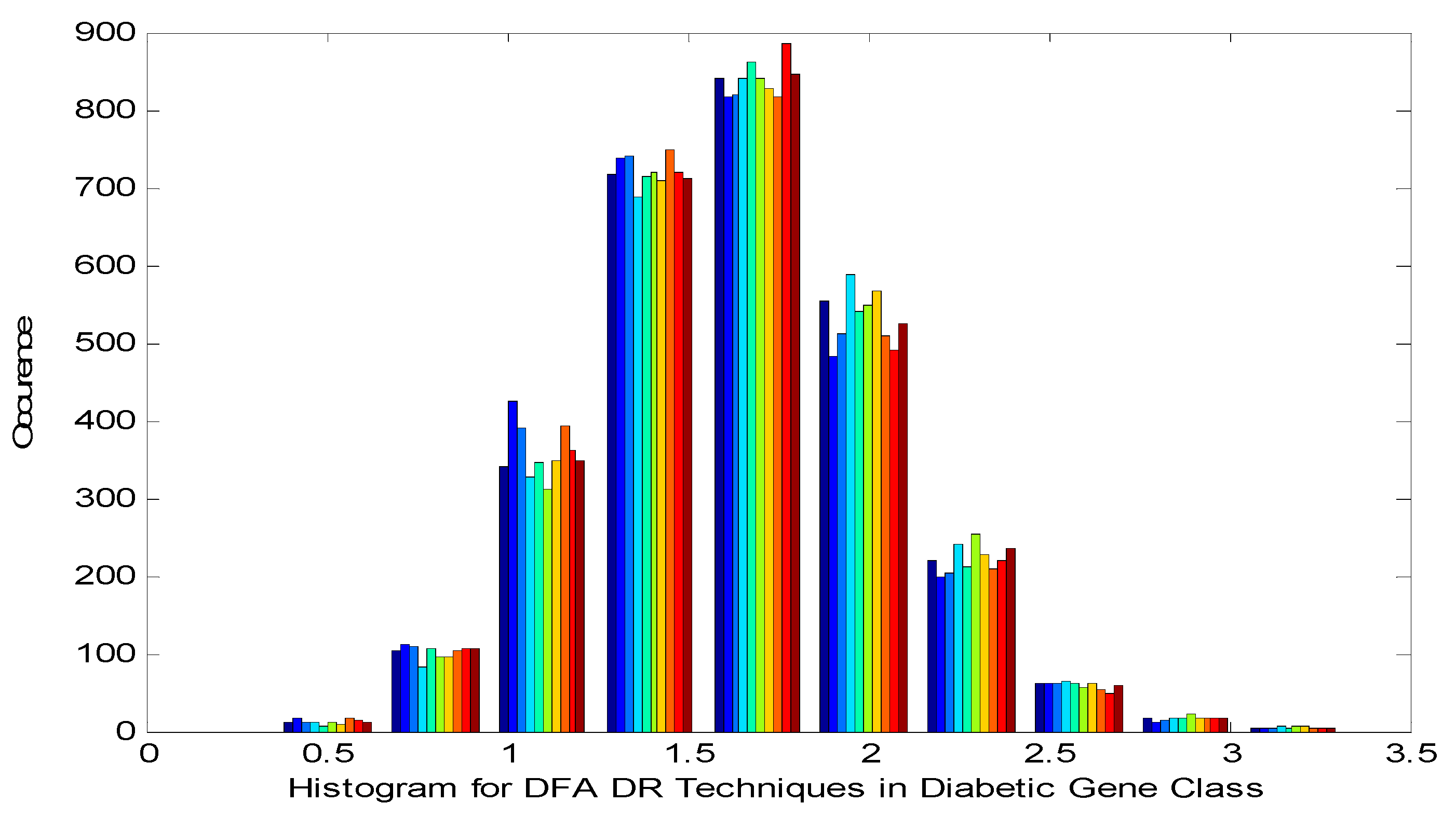
Figure 3.
Histogram of Detrend Fluctuation Analysis (DFA) Techniques in Normal Gene Class.
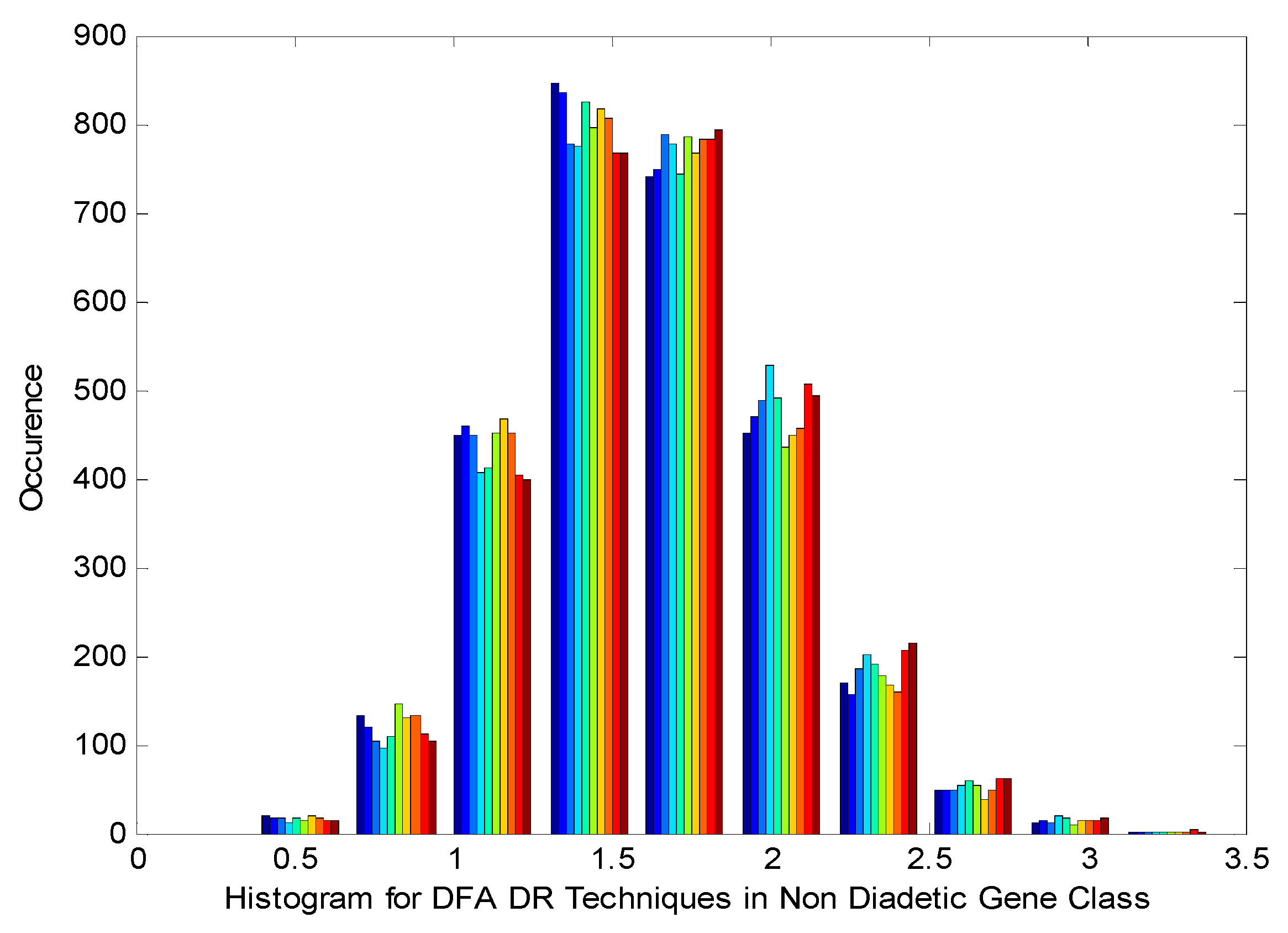
Figure 4.
Normal Probability plot for Chi Square DR Techniques Features for Diabetic Gene Class.
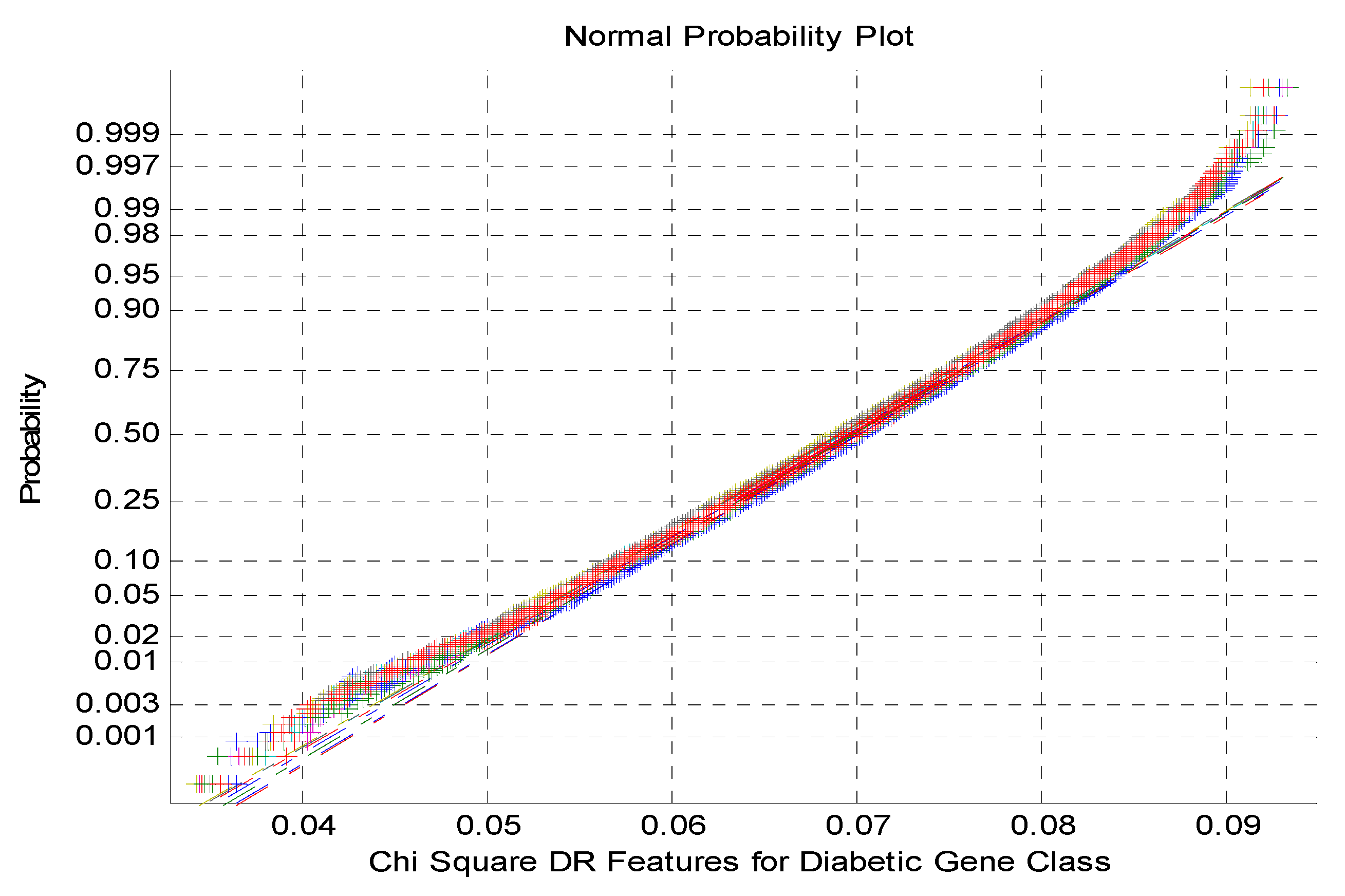
Figure 5.
Normal Probability plot for Chi Square DR Techniques Features for Non-Diabetic Gene Class.
Figure 5.
Normal Probability plot for Chi Square DR Techniques Features for Non-Diabetic Gene Class.
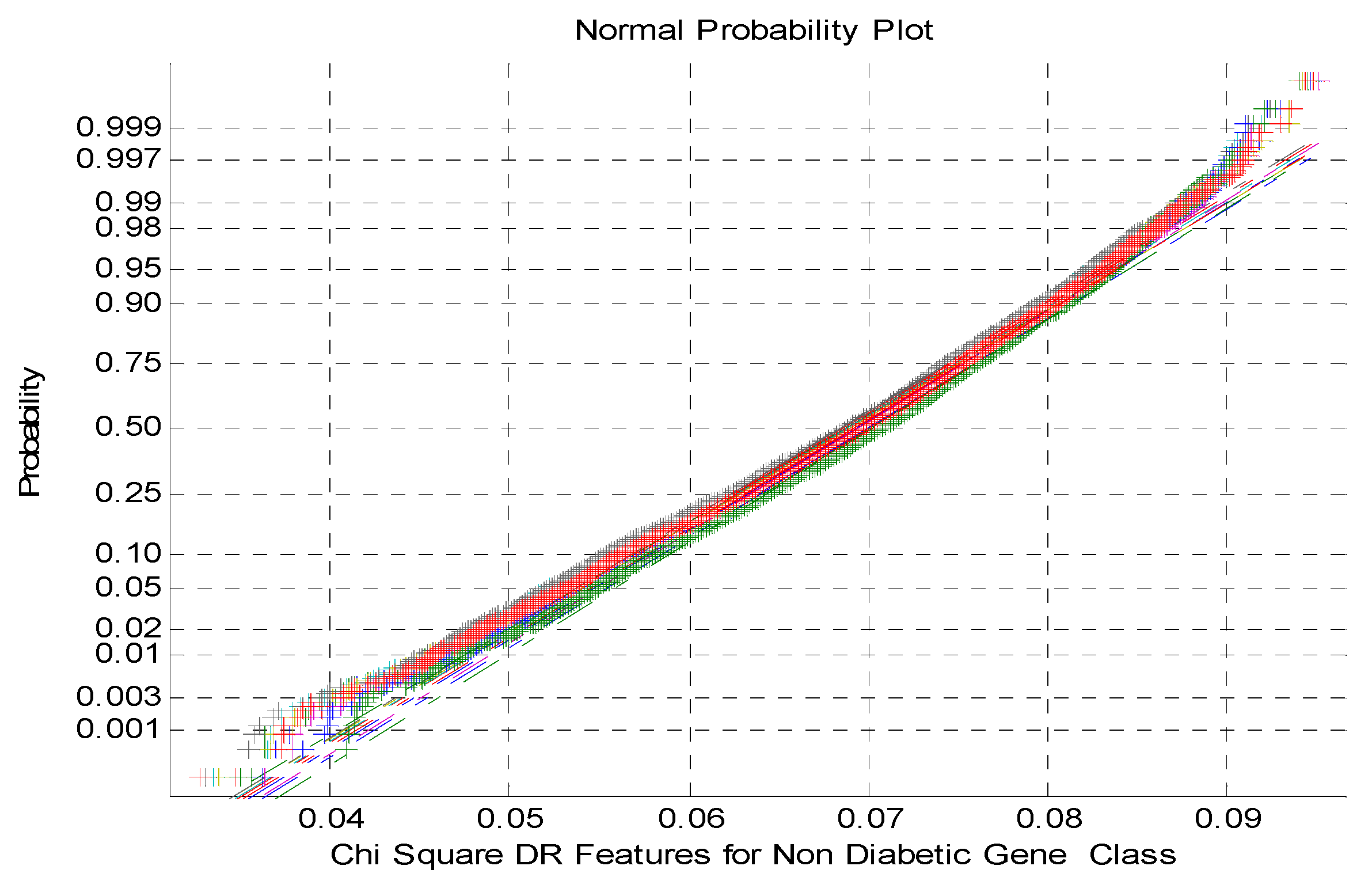
Figure 6.
Normal Probability plot for Firefly Algorithm DR Techniques Features for Diabetic Gene Class.
Figure 6.
Normal Probability plot for Firefly Algorithm DR Techniques Features for Diabetic Gene Class.
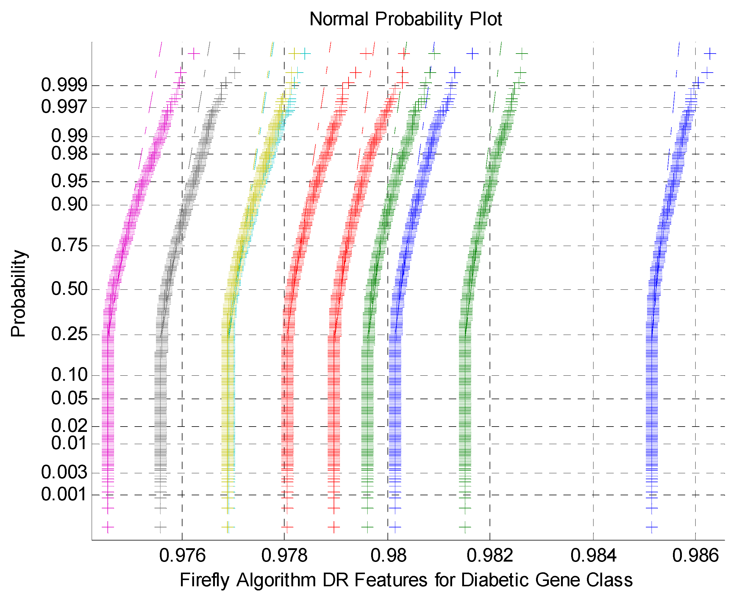
Figure 7.
Normal Probability plot for Firefly Algorithm DR Techniques Features for Non-Diabetic Gene Class.
Figure 7.
Normal Probability plot for Firefly Algorithm DR Techniques Features for Non-Diabetic Gene Class.
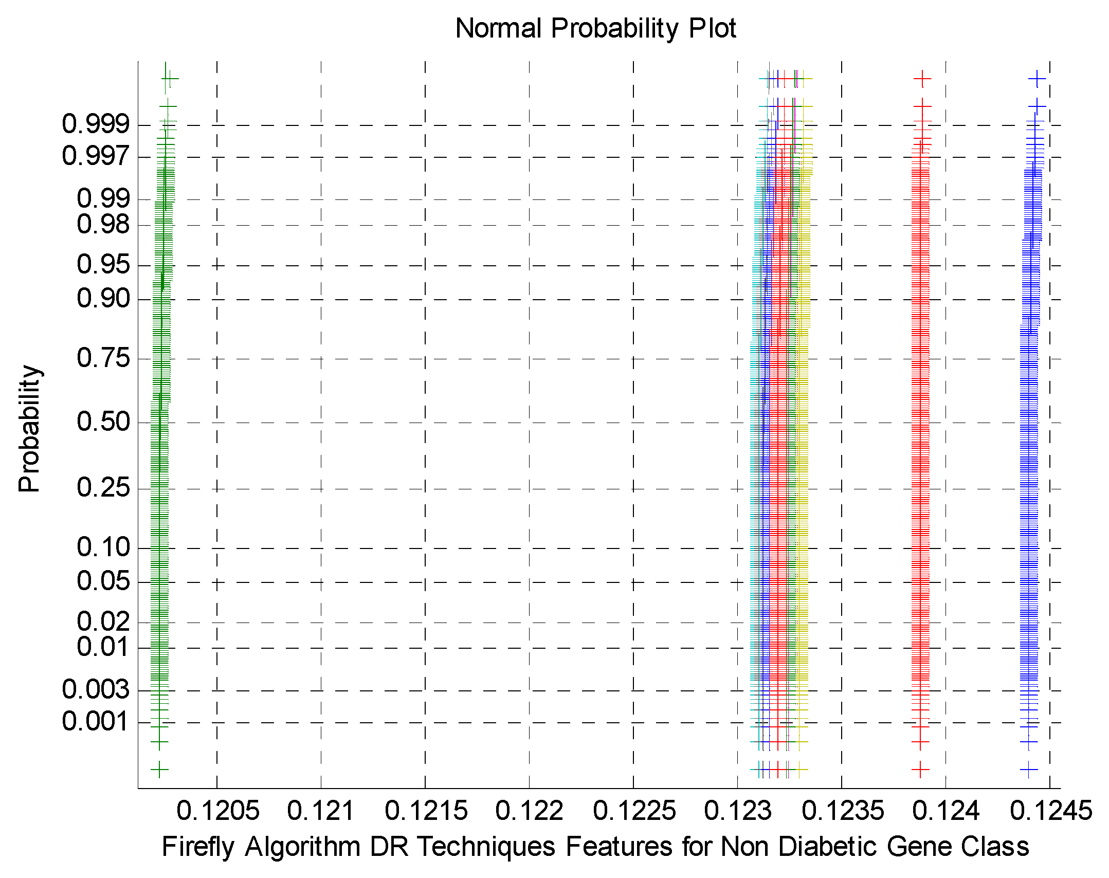
Figure 8.
Scatter plot for Cuckoo search DR Technique with Diabetic and Non-Diabetic Gene classes.
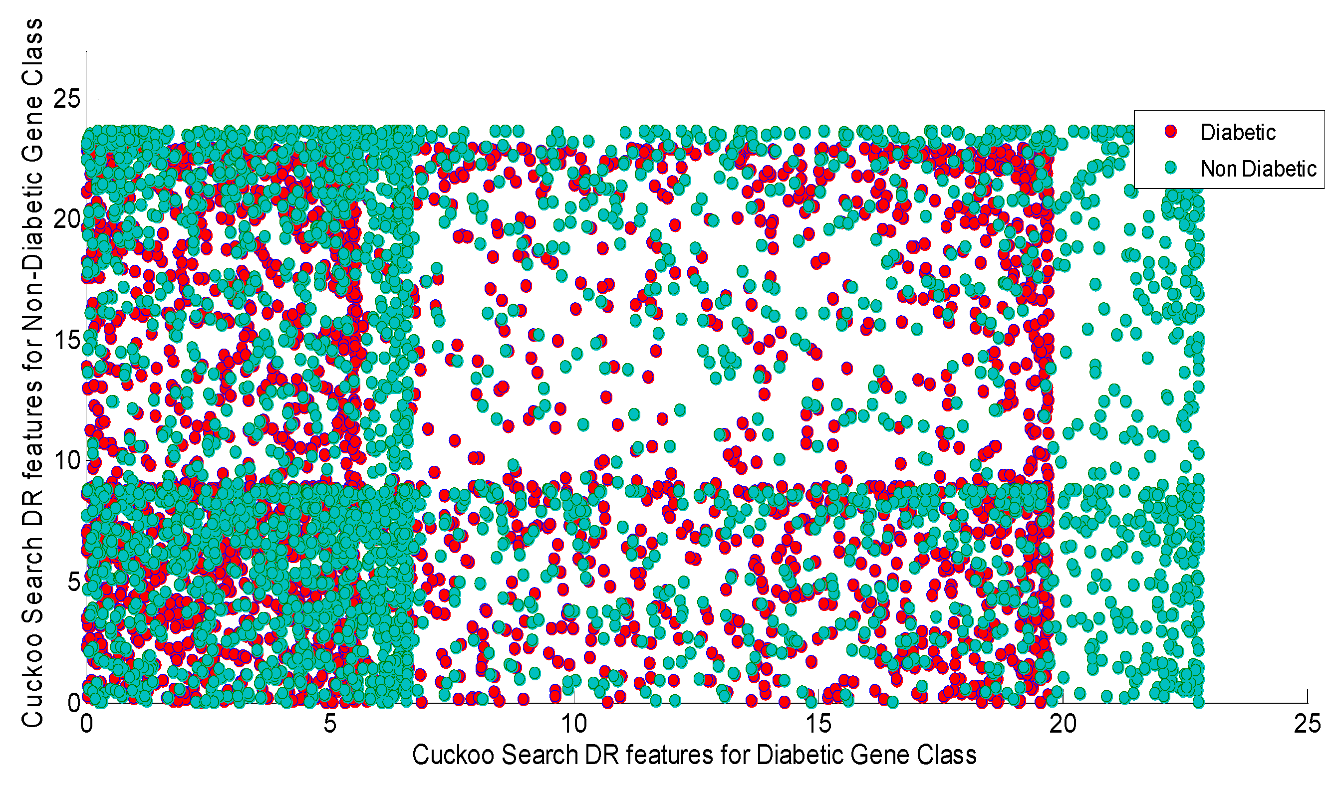
Figure 9.
Performance Analysis of Classifiers without Feature Selection Methods.
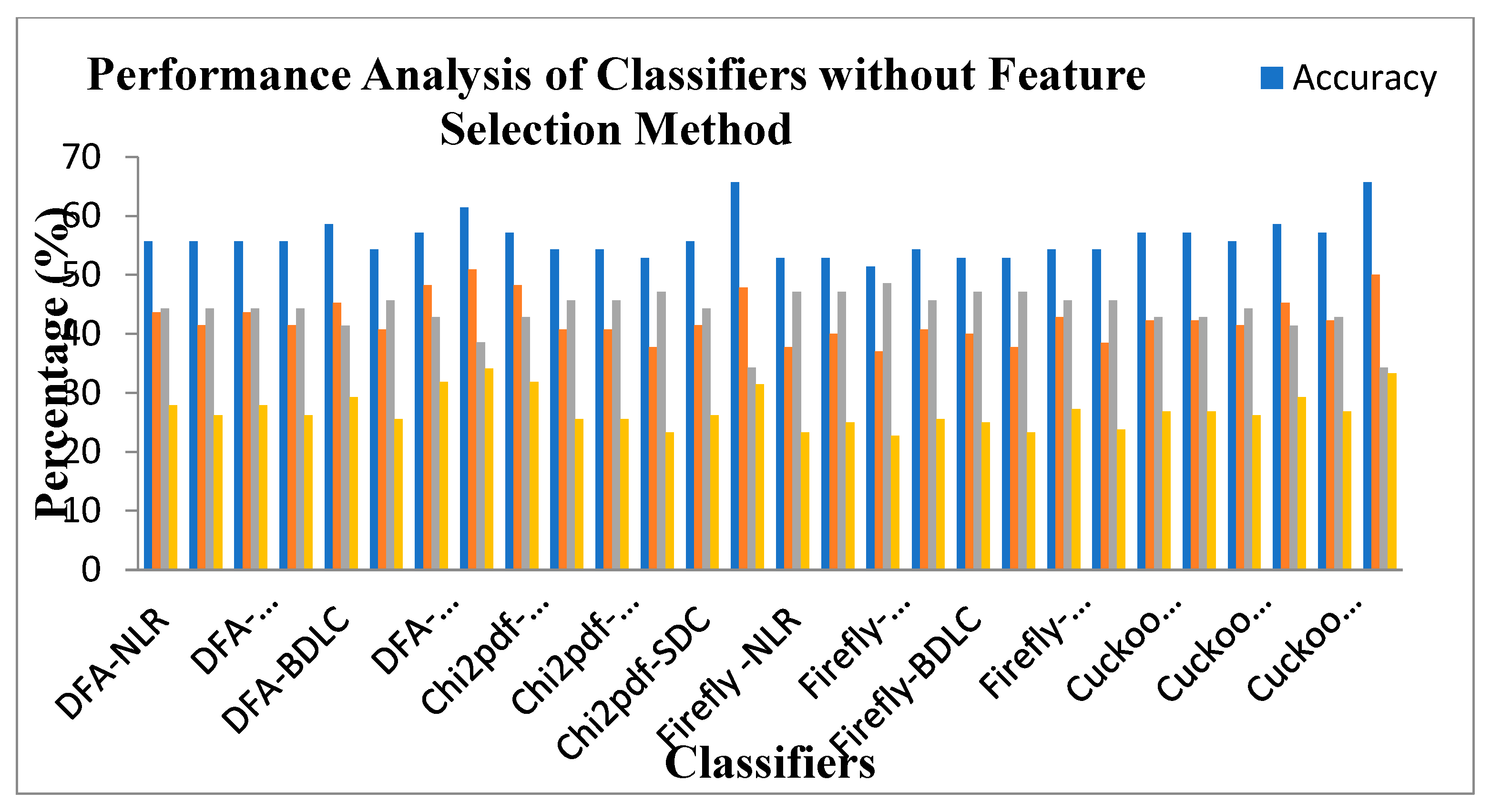
Figure 10.
Performance Analysis of Classifiers with PSO Feature Selection Methods.
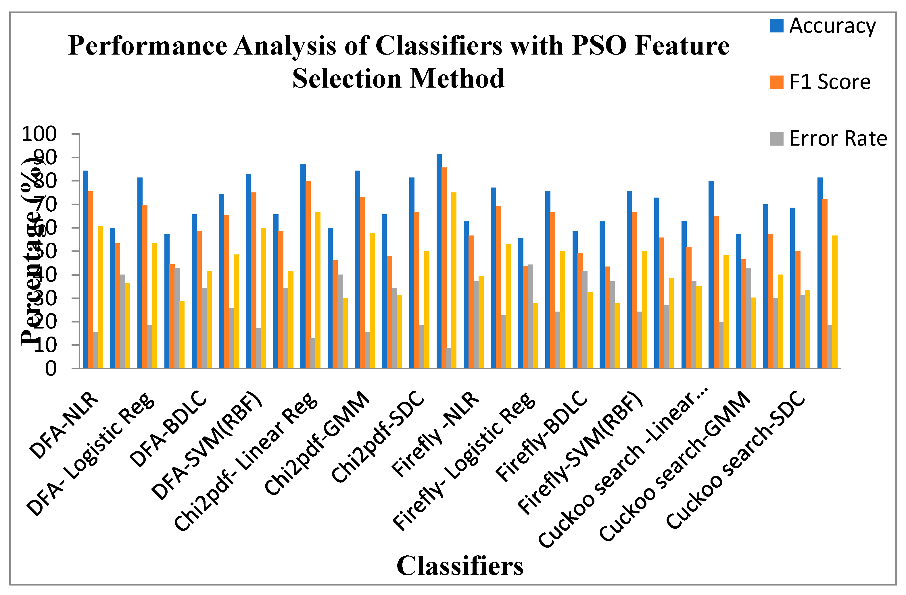
Figure 11.
Performance Analysis of Classifiers with Harmonic Search Feature Selection Methods.
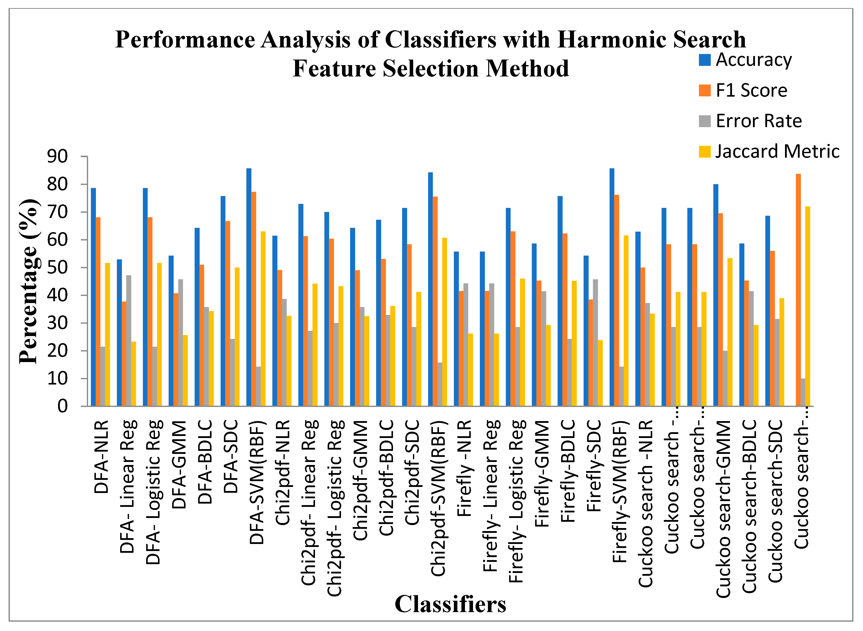
Figure 12.
Performance of MCC and Kappa Parameters across the classifier for four DR Techniques without and with Two Feature Selection Methods.
Figure 12.
Performance of MCC and Kappa Parameters across the classifier for four DR Techniques without and with Two Feature Selection Methods.
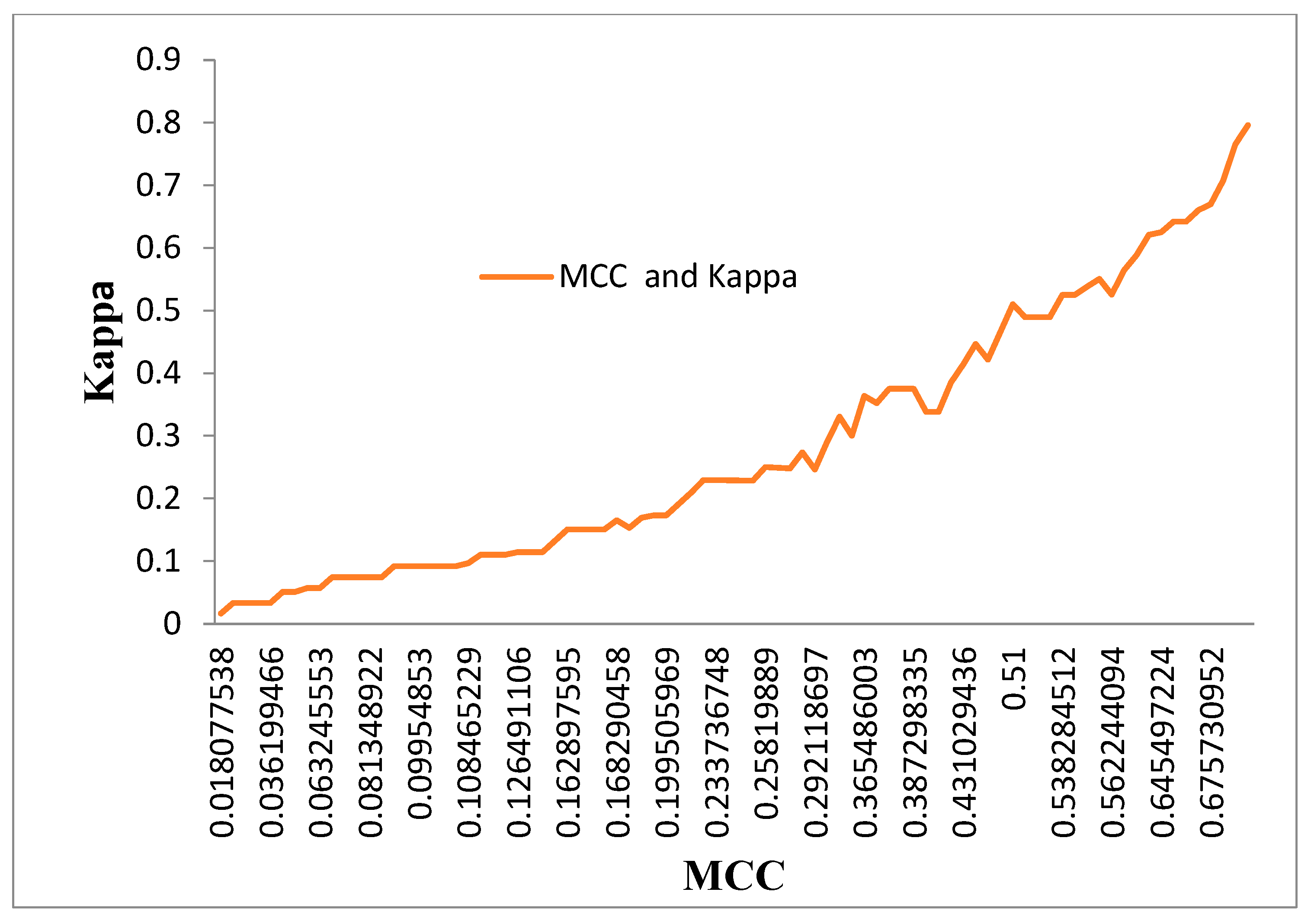
Table 1.
Description of Pancreas Micro Array Gene Data set for Diabetic and Non-Diabetic Classes.
| Data Set | No of Genes | Class 1 Diabetes |
Class 2 Non - Diabetic |
Total |
|---|---|---|---|---|
| Pancreas | 28735 | 20 | 50 | 70 |
Table 2.
Statistical Analysis for Different Dimensionality Reduction Techniques.
| Statistical Parameters | DFA | Chi2 pdf | Firefly Algorithm |
Cuckoo Search |
||||
|---|---|---|---|---|---|---|---|---|
| DP | NDP | DP | NDP | DP | NDP | DP | NDP | |
| Mean | 1.6302 | 1.6301 | 0.0690 | 0.0691 | 1.0278 | 0.1260 | 8.7158 | 12.6033 |
| Variance | 0.1614 | 0.1665 | 0.0007 | 0.0008 | 0.0004 | 1.45 E-09 | 48.4751 | 71.7672 |
| Skewness | 0.2319 | 0.2758 | -0.2771 | -0.3228 | 1.6527 | 4.0298 | 0.6087 | 0.2692 |
| Kurtosis | 0.2706 | 0.1600 | 0.0301 | 0.0096 | 3.1033 | 78.3911 | -1.1233 | -1.3759 |
| Pearson CC | 0.9516 | 0.9598 | 0.9781 | 0.9814 | 0.8803 | 0.5006 | 0.7048 | 0.6859 |
| CCA | 0.05914 | 0.06411 | 0.04785 | 0.05107 | ||||
Table 3.
P-Value significant for Feature Selection method from t-test for different DR Techniques.
| Feature selection | DR Techniques | DFA | Chi Square pdf | Firefly Algorithm |
Cuckoo Search | ||||
|---|---|---|---|---|---|---|---|---|---|
| Class | DP | NDP | DP | NDP | DP | NDP | DP | NDP | |
| PSO | P value <0.05 |
0.415 | 0.1906 | 0.3877 | 0.16074 | 0.38059 | 0.2435 | 0.4740 | 0.48824 |
| Harmonic Search | P value <0.05 |
0.0004 | 0.4290 | 0.3836 | 0.43655 | 0.00031 | 0.469 | 0.3488 | 0 .3979 |
Table 5.
exhibits the training and testing MSE performance of the classifiers without feature selection Method for four Dimensionality Reduction Techniques.
Table 5.
exhibits the training and testing MSE performance of the classifiers without feature selection Method for four Dimensionality Reduction Techniques.
| Classifiers | With DFA DR Method |
With Chi2 pdf DR Method |
With Firefly Algorithm DR Method |
Cuckoo Search DR Method |
||||
|---|---|---|---|---|---|---|---|---|
| Training MSE |
Testing MSE |
Training MSE |
Testing MSE |
Training MSE | Testing MSE |
Training MSE |
Testing MSE |
|
| NLR | 7.92E-05 | 0.0001633 | 9.8E-05 | 5.439E-05 | 6.56E-05 | 0.00029 | 2.81E-05 | 0.000145 |
| Linear Reg | 4.62E-05 | 8.936E-05 | 6.08E-05 | 0.0001945 | 5.48E-05 | 0.0003566 | 9.22E-05 | 0.000135 |
| Logistic Regression | 2.6E-05 | 0.0001325 | 2.21E-05 | 0.0001565 | 8.84E-05 | 0.0004625 | 9.8E-05 | 0.0001685 |
| GMM | 1.52E-05 | 0.000121 | 7.06E-05 | 0.0001662 | 7.92E-05 | 0.0002442 | 0.0000342 | 0.0001103 |
| BDLC | 0.00000182 | 6.978E-05 | 8.46E-05 | 0.0002492 | 4.49E-05 | 0.0002136 | 0.0000144 | 7.161E-05 |
| SDC | 0.0000272 | 0.0001567 | 0.0000121 | 0.0001095 | 4.22E-05 | 0.0003081 | 0.0000121 | 0.000104 |
| SVM(RBF) | 0.0000196 | 0.0001656 | 4.62E-05 | 0.0001454 | 3.48E-05 | 0.0001924 | 1.26 E-08 | 5.141E-06 |
Table 6.
Training and Testing MSE Analysis of Classifiers for Various Dimensionality Reduction Technique with PSO Feature Selection Methods.
Table 6.
Training and Testing MSE Analysis of Classifiers for Various Dimensionality Reduction Technique with PSO Feature Selection Methods.
| Classifiers | With DFA DR Method |
With Chi2 pdf DR Method |
With Firefly Algorithm DR Method |
Cuckoo Search DR Method |
||||
|---|---|---|---|---|---|---|---|---|
| Training MSE |
Testing MSE | Training MSE |
Testing MSE |
Training MSE |
Testing MSE |
Training MSE |
Testing MSE |
|
| NLR | 3.61E-06 | 9.01E-06 | 5.29E-06 | 4.062E-05 | 3.36E-05 | 0.0001568 | 3.84E-07 | 3.737E-05 |
| Linear Reg | 9.61E-06 | 0.0001603 | 1.22E-07 | 4.825E-06 | 8.28E-06 | 1.464E-05 | 4.62E-06 | 5.042E-05 |
| Logistic Regression | 1.44E-05 | 1.422E-05 | 2.6E-08 | 6.806E-05 | 6.89E-05 | 0.0001486 | 7.4E-07 | 2.906E-05 |
| GMM | 6.24E-05 | 8.021E-05 | 1.36E-07 | 1.168E-05 | 4.62E-06 | 1.394E-05 | 2.7E-05 | 0.0001511 |
| BDLC | 1.76E-05 | 4.063E-05 | 7.29E-06 | 5.653E-05 | 1.52E-06 | 0.0001192 | 5.33E-07 | 2.92E-05 |
| SDC | 9E-06 | 2.005E-05 | 2.89E-06 | 2.493E-05 | 1.02E-05 | 0.0001243 | 8.65E-08 | 5.525E-05 |
| SVM(RBF) | 2.12E-07 | 8.5E-06 | 1.94E-09 | 1.885E-06 | 2.56E-06 | 1.889E-05 | 7.22E-07 | 1.022E-05 |
Table 7.
Training and Testing MSE Analysis of Classifiers for Various Dimensionality Reduction Technique with Harmonic Search Feature Selection Methods.
Table 7.
Training and Testing MSE Analysis of Classifiers for Various Dimensionality Reduction Technique with Harmonic Search Feature Selection Methods.
| Classifiers | With DFA DR Method |
With Chi2 pdf DR Method |
With Firefly Algorithm DR Method | Cuckoo Search DR Method |
||||
|---|---|---|---|---|---|---|---|---|
| Training MSE | Testing MSE | Training MSE | Testing MSE | Training MSE | Testing MSE | Training MSE | Testing MSE | |
| NLR | 7.06E-05 | 1.68E-05 | 3.25E-05 | 5.46E-05 | 5.04E-05 | 9.7E-05 | 9.61E-06 | 5.07E-05 |
| Linear Reg | 9.22E-05 | 0.000244 | 1.44E-05 | 2.22E-05 | 1.68E-05 | 0.000121 | 8.28E-07 | 2.86E-05 |
| Logistic Regression | 5.93E-08 | 1.68E-05 | 6.25E-06 | 3.03E-05 | 2.81E-07 | 2.86E-05 | 3.25E-05 | 3.14E-05 |
| GMM | 1.09E-05 | 0.000221 | 1.76E-05 | 5.66E-05 | 3.02E-05 | 7.57E-05 | 3.84E-05 | 1.23E-05 |
| BDLC | 2.92E-08 | 5.04E-05 | 0.000182 | 4.22E-05 | 3.25E-05 | 2.58E-05 | 1.85E-05 | 7.42E-05 |
| SDC | 6.56E-05 | 1.72E-05 | 0.000169 | 2.5E-05 | 5.76E-06 | 0.000225 | 1.52E-05 | 3.72E-05 |
| SVM(RBF) | 4.36E-05 | 4.88E-06 | 7.4E-05 | 8.13E-06 | 6.56E-05 | 1.02E-05 | 1.86E-08 | 1.7E-06 |
Table 9.
Average Performance of Classifiers with different DM techniques Without Feature Selection Methods.
Table 9.
Average Performance of Classifiers with different DM techniques Without Feature Selection Methods.
| Dimensionality Reduction | Classifiers | Parameters | |||||
|---|---|---|---|---|---|---|---|
| Accuracy (%) |
F1Score (%) |
MCC | Error Rate (%) |
Jaccard Metric (%) |
Kappa | ||
| Detrend Fluctuation Analysis (DFA) | NLR | 55.71429 | 43.63636 | 0.126491 | 44.28571 | 27.90697674 | 0.114286 |
| Linear Reg | 55.71429 | 41.50943 | 0.099549 | 44.28571 | 26.19047619 | 0.09205 | |
| Logistic Regression | 55.71429 | 43.63636 | 0.126491 | 44.28571 | 27.90697674 | 0.114286 | |
| GMM | 55.71429 | 41.50943 | 0.099549 | 44.28571 | 26.19047619 | 0.09205 | |
| BDLC | 58.57143 | 45.28302 | 0.162898 | 41.42857 | 29.26829268 | 0.150628 | |
| SDC | 54.28571 | 40.74074 | 0.081349 | 45.71429 | 25.58139535 | 0.07438 | |
| SVM(RBF) | 57.14286 | 48.27586 | 0.199506 | 42.85714 | 31.81818182 | 0.173228 | |
| Chi2pdf | NLR | 61.42857 | 50.90909 | 0.252982 | 38.57143 | 34.14634146 | 0.228571 |
| Linear Reg | 57.14286 | 48.27586 | 0.199506 | 42.85714 | 31.81818182 | 0.173228 | |
| Logistic Regression | 54.28571 | 40.74074 | 0.081349 | 45.71429 | 25.58139535 | 0.07438 | |
| GMM | 54.28571 | 40.74074 | 0.081349 | 45.71429 | 25.58139535 | 0.07438 | |
| BDLC | 52.85714 | 37.73585 | 0.036199 | 47.14286 | 23.25581395 | 0.033473 | |
| SDC | 55.71429 | 41.50943 | 0.099549 | 44.28571 | 26.19047619 | 0.09205 | |
| SVM(RBF) | 65.71429 | 47.82609 | 0.233737 | 34.28571 | 31.42857143 | 0.229358 | |
| Firefly Algorithm | NLR | 52.85714 | 37.73585 | 0.036199 | 47.14286 | 23.25581395 | 0.033473 |
| Linear Reg | 52.85714 | 40 | 0.063246 | 47.14286 | 25 | 0.057143 | |
| Logistic Regression | 51.42857 | 37.03704 | 0.018078 | 48.57143 | 22.72727273 | 0.016529 | |
| GMM | 54.28571 | 40.74074 | 0.081349 | 45.71429 | 25.58139535 | 0.07438 | |
| BDLC | 52.85714 | 40 | 0.063246 | 47.14286 | 25 | 0.057143 | |
| SDC | 52.85714 | 37.73585 | 0.036199 | 47.14286 | 23.25581395 | 0.033473 | |
| SVM(RBF) | 54.28571 | 42.85714 | 0.108465 | 45.71429 | 27.27272727 | 0.096774 | |
| Cuckoo Search | NLR | 54.28571 | 38.46154 | 0.054411 | 45.71429 | 23.80952381 | 0.050847 |
| Linear Reg | 57.14286 | 42.30769 | 0.11789 | 42.85714 | 26.82926829 | 0.110169 | |
| Logistic Regression | 57.14286 | 42.30769 | 0.11789 | 42.85714 | 26.82926829 | 0.110169 | |
| GMM | 55.71429 | 41.50943 | 0.099549 | 44.28571 | 26.19047619 | 0.09205 | |
| BDLC | 58.57143 | 45.28302 | 0.162898 | 41.42857 | 29.26829268 | 0.150628 | |
| SDC | 57.14286 | 42.30769 | 0.11789 | 42.85714 | 26.82926829 | 0.110169 | |
| SVM(RBF) | 65.71429 | 50 | 0.258199 | 34.28571 | 33.33333333 | 0.25 | |
Table 10.
Average Performance of Classifiers with different DM techniques With PSO Feature Selection Method.
Table 10.
Average Performance of Classifiers with different DM techniques With PSO Feature Selection Method.
| Dimensionality Reduction | Classifiers | Parameters | |||||
|---|---|---|---|---|---|---|---|
| Accuracy (%) |
F1Score (%) |
MCC | Error Rate (%) |
Jaccard Metric (%) |
Kappa | ||
| Detrend Fluctuation Analysis (DFA) | NLR | 84.28571 | 75.55556 | 0.650538 | 15.71429 | 60.71428571 | 0.64186 |
| Linear Reg | 60 | 53.33333 | 0.292119 | 40 | 36.36363636 | 0.246154 | |
| Logistic Regression | 81.42857 | 69.76744 | 0.567465 | 18.57143 | 53.57142857 | 0.564593 | |
| GMM | 57.14286 | 44.44444 | 0.14462 | 42.85714 | 28.57142857 | 0.132231 | |
| BDLC | 65.71429 | 58.62069 | 0.389943 | 34.28571 | 41.46341463 | 0.338583 | |
| SDC | 74.28571 | 65.38462 | 0.498765 | 25.71429 | 48.57142857 | 0.466102 | |
| SVM(RBF) | 82.85714 | 75 | 0.645497 | 17.14286 | 60 | 0.625 | |
| Chi2pdf | NLR | 65.71429 | 58.62069 | 0.389943 | 34.28571 | 41.46341463 | 0.338583 |
| Linear Reg | 87.14286 | 80 | 0.716535 | 12.85714 | 66.66666667 | 0.706977 | |
| Logistic Regression | 60 | 46.15385 | 0.181369 | 40 | 30 | 0.169492 | |
| GMM | 84.28571 | 73.17073 | 0.621059 | 15.71429 | 57.69230769 | 0.62069 | |
| BDLC | 65.71429 | 47.82609 | 0.233737 | 34.28571 | 31.42857143 | 0.229358 | |
| SDC | 81.42857 | 66.66667 | 0.538411 | 18.57143 | 50 | 0.538071 | |
| SVM(RBF) | 91.42857 | 85.71429 | 0.797961 | 8.571429 | 75 | 0.796117 | |
| Firefly Algorithm | NLR | 62.85714 | 56.66667 | 0.35602 | 37.14286 | 39.53488372 | 0.3 |
| Linear Reg | 77.14286 | 69.23077 | 0.562244 | 22.85714 | 52.94117647 | 0.525424 | |
| Logistic Regression | 55.71429 | 43.63636 | 0.126491 | 44.28571 | 27.90697674 | 0.114286 | |
| GMM | 75.71429 | 66.66667 | 0.518396 | 24.28571 | 50 | 0.48927 | |
| BDLC | 58.57143 | 49.12281 | 0.217197 | 41.42857 | 32.55813953 | 0.191235 | |
| SDC | 62.85714 | 43.47826 | 0.16829 | 37.14286 | 27.77777778 | 0.165138 | |
| SVM(RBF) | 75.71429 | 66.66667 | 0.518396 | 24.28571 | 50 | 0.48927 | |
| Cuckoo Search | NLR | 72.85714 | 55.81395 | 0.365486 | 27.14286 | 38.70967742 | 0.363636 |
| Linear Reg | 62.85714 | 51.85185 | 0.271163 | 37.14286 | 35 | 0.247934 | |
| Logistic Regression | 80 | 65 | 0.51 | 20 | 48.14814815 | 0.51 | |
| GMM | 57.14286 | 46.42857 | 0.171737 | 42.85714 | 30.23255814 | 0.153226 | |
| BDLC | 70 | 57.14286 | 0.366834 | 30 | 40 | 0.352423 | |
| SDC | 68.57143 | 50 | 0.276003 | 31.42857 | 33.33333333 | 0.273585 | |
| SVM(RBF) | 81.42857 | 72.34043 | 0.60325 | 18.57143 | 56.66666667 | 0.588235 | |
Table 11.
Average Performance of Classifiers with different DM techniques With Harmonic Search Feature Selection Method.
Table 11.
Average Performance of Classifiers with different DM techniques With Harmonic Search Feature Selection Method.
| Dimensionality Reduction | Classifiers | Parameters | |||||
|---|---|---|---|---|---|---|---|
| Accuracy (%) |
F1Score (%) |
MCC | Error Rate (%) |
Jaccard Metric (%) |
Kappa | ||
| Detrend Fluctuation Analysis (DFA) | NLR | 78.57143 | 68.08511 | 0.538285 | 21.42857 | 51.6129 | 0.524887 |
| Linear Reg | 52.85714 | 37.73585 | 0.036199 | 47.14286 | 23.25581 | 0.033473 | |
| Logistic Regression | 78.57143 | 68.08511 | 0.538285 | 21.42857 | 51.6129 | 0.524887 | |
| GMM | 54.28571 | 40.74074 | 0.081349 | 45.71429 | 25.5814 | 0.07438 | |
| BDLC | 64.28571 | 50.98039 | 0.263745 | 35.71429 | 34.21053 | 0.248927 | |
| SDC | 75.71429 | 66.66667 | 0.518396 | 24.28571 | 50 | 0.48927 | |
| SVM(RBF) | 85.71429 | 77.27273 | 0.675731 | 14.28571 | 62.96296 | 0.669811 | |
| Chi2pdf | NLR | 61.42857 | 49.0566 | 0.226247 | 38.57143 | 32.5 | 0.209205 |
| Linear Reg | 72.85714 | 61.22449 | 0.431029 | 27.14286 | 44.11765 | 0.414097 | |
| Logistic Regression | 70 | 60.37736 | 0.416294 | 30 | 43.24324 | 0.384937 | |
| GMM | 64.28571 | 48.97959 | 0.238442 | 35.71429 | 32.43243 | 0.229075 | |
| BDLC | 67.14286 | 53.06122 | 0.302638 | 32.85714 | 36.11111 | 0.290749 | |
| SDC | 71.42857 | 58.33333 | 0.387298 | 28.57143 | 41.17647 | 0.375 | |
| SVM(RBF) | 84.28571 | 75.55556 | 0.650538 | 15.71429 | 60.71429 | 0.64186 | |
| Firefly Algorithm | NLR | 55.71429 | 41.50943 | 0.099549 | 44.28571 | 26.19048 | 0.09205 |
| Linear Reg | 55.71429 | 41.50943 | 0.099549 | 44.28571 | 26.19048 | 0.09205 | |
| Logistic Regression | 71.42857 | 62.96296 | 0.460977 | 28.57143 | 45.94595 | 0.421488 | |
| GMM | 58.57143 | 45.28302 | 0.162898 | 41.42857 | 29.26829 | 0.150628 | |
| BDLC | 75.71429 | 62.22222 | 0.452548 | 24.28571 | 45.16129 | 0.446512 | |
| SDC | 54.28571 | 38.46154 | 0.054411 | 45.71429 | 23.80952 | 0.050847 | |
| SVM(RBF) | 85.71429 | 76.19048 | 0.661724 | 14.28571 | 61.53846 | 0.660194 | |
| Cuckoo Search | NLR | 62.85714 | 50 | 0.244848 | 37.14286 | 33.33333 | 0.228814 |
| Linear Reg | 71.42857 | 58.33333 | 0.387298 | 28.57143 | 41.17647 | 0.375 | |
| Logistic Regression | 71.42857 | 58.33333 | 0.387298 | 28.57143 | 41.17647 | 0.375 | |
| GMM | 80 | 69.56522 | 0.560968 | 20 | 53.33333 | 0.550459 | |
| BDLC | 58.57143 | 45.28302 | 0.162898 | 41.42857 | 29.26829 | 0.150628 | |
| SDC | 68.57143 | 56 | 0.346891 | 31.42857 | 38.88889 | 0.330435 | |
| SVM(RBF) | 90 | 83.72093 | 0.769444 | 10 | 72 | 0.76555 | |
Table 12.
Computational Complexity of the Classifiers for Different Dimensionality Reduction Method without Feature selection methods.
Table 12.
Computational Complexity of the Classifiers for Different Dimensionality Reduction Method without Feature selection methods.
| Classifiers | With DFA DR Method | With Chi2 pdf DR Method | With Firefly Algorithm DR Method | Cuckoo Search DR Method |
|---|---|---|---|---|
| NLR | O(2n2 log2n) | O(2n2 log 2n) | O(2n4 log 2n) | O(2n4 log2n) |
| Linear Reg | O(2n log2n) | O(2n2 log 2n) | O(2n3 log 2n) | O(2n3log2n) |
| Logistic Regression | O(2n2 log2n) | O(2n2 log 2n) | O(2n3 log 2n) | O(2n3 log2n) |
| GMM | O(2n3 log2n) | O(2n3 log 2n) | O(2n4 log 2n) | O(2n4 log2n) |
| BDLC | O(2n3 log2n) | O(2n3 log 2n) | O(2n4 log 2n) | O(2n4 log2n) |
| SDC | O(2n2 log2n) | O(2n2 log 2n) | O(2n4 log 2n) | O(2n4 log2n) |
| SVM(RBF) | O(2n2 log4n) | O(2n2 log 4n) | O(2n4 log 4n) | O(2n3 log4n) |
Table 13.
Computational Complexity of the Classifiers for Different Dimensionality Reduction Method with PSO Feature selection method.
Table 13.
Computational Complexity of the Classifiers for Different Dimensionality Reduction Method with PSO Feature selection method.
| Classifiers | With DFA DR Method |
With Chi2 pdf DR Method |
With Firefly Algorithm DR Method |
Cuckoo Search DR Method |
|---|---|---|---|---|
| NLR | O(2n4 log2n) | O(2n4 log 2n) | O(2n6 log 2n) | O(2n6 log2n) |
| Linear Reg | O(2n3 log2n) | O(2n4 log 2n) | O(2n5 log 2n) | O(2n5log2n) |
| Logistic Regression | O(2n4 log2n) | O(2n4 log 2n) | O(2n4 log 2n) | O(2n5 log2n) |
| GMM | O(2n5 log2n) | O(2n5 log 2n) | O(2n6 log 2n) | O(2n6 log2n) |
| BDLC | O(2n5 log2n) | O(2n5 log 2n) | O(2n6 log 2n) | O(2n6 log2n) |
| SDC | O(2n4 log2n) | O(2n4 log 2n) | O(2n4 log 2n) | O(2n4 log2n) |
| SVM(RBF) | O(2n4 log2n) | O(2n4 log 4n) | O(2n6 log 4n) | O(2n5 log4n) |
Table 14.
Computational Complexity of the Classifiers for Different Dimensionality Reduction Method with Harmonic Search Feature selection method.
Table 14.
Computational Complexity of the Classifiers for Different Dimensionality Reduction Method with Harmonic Search Feature selection method.
| Classifiers | With DFA DR Method |
With Chi2 pdf DR Method |
With Firefly Algorithm DR Method |
Cuckoo Search DR Method |
|---|---|---|---|---|
| NLR | O(2n3 log2n) | O(2n3 log 2n) | O(2n4 log 2n) | O(2n4 log2n) |
| Linear Reg | O(2n2 log2n) | O(2n3 log 2n) | O(2n5 log 2n) | O(2n5log2n) |
| Logistic Regression | O(2n3 log2n) | O(2n3 log 2n) | O(2n4 log 2n) | O(2n4 log2n) |
| GMM | O(2n4 log2n) | O(2n5log 2n) | O(2n5 log 2n) | O(2n5 log2n) |
| BDLC | O(2n4 log2n) | O(2n4 log 2n) | O(2n5 log 2n) | O(2n5 log2n) |
| SDC | O(2n3 log2n) | O(2n3log 2n) | O(2n3 log 2n) | O(2n4 log2n) |
| SVM(RBF) | O(2n4 log2n) | O(2n4 log 2n) | O(2n4 log 2n) | O(2n4 log2n) |
Disclaimer/Publisher’s Note: The statements, opinions and data contained in all publications are solely those of the individual author(s) and contributor(s) and not of MDPI and/or the editor(s). MDPI and/or the editor(s) disclaim responsibility for any injury to people or property resulting from any ideas, methods, instructions or products referred to in the content. |
© 2023 by the authors. Licensee MDPI, Basel, Switzerland. This article is an open access article distributed under the terms and conditions of the Creative Commons Attribution (CC BY) license (http://creativecommons.org/licenses/by/4.0/).
Copyright: This open access article is published under a Creative Commons CC BY 4.0 license, which permit the free download, distribution, and reuse, provided that the author and preprint are cited in any reuse.


