Has the Problem of the Motion of a Heavy Symmetric Top Been Solved in Quadratures?

Alexei A. Deriglazov

doi:10.20944/preprints202306.0702.v1

Submitted:

08 June 2023

Posted:

09 June 2023

You are already at the latest version

Abstract

We have revised the problem of the motion of a heavy symmetric top. When formulating equations of motion of the Lagrange top with the diagonal inertia tensor, the potential energy has more complicated form as compared with that assumed in the literature on dynamics of a rigid body. Using the Liouville's theorem, we solve the improved equations in quadratures and present the explicit expressions for the resulting elliptic integrals.

Keywords:

Integrability

;

Lagrange top

;

Hamiltonian systems

;

Liouville's theorem

Subject:

Physical Sciences - Mathematical Physics

I. Introduction

This paper is the fifth in the series [1,2,3,4], devoted to a systematic exposition of the dynamics of a rigid body, considered as a system with kinematic constraints. In the previous works has been considered the dynamics of a free asymmetric body. Here we revise the problem of the motion of inclined heavy symmetric top with one fixed point.

Free asymmetric body. The evolution of a free rigid body in the center-of-mass system can be described by

3 + 9

Euler-Poisson equations [1]

\begin{matrix} I \dot{Ω} = [I Ω, Ω], {\dot{R}}_{i j} = - ϵ_{j k m} Ω_{k} R_{i m} . \end{matrix}

(1)

Here the functions

Ω_{i} (t)

are components of angular velocity in the body, and

R_{i j} (t)

is orthogonal

3 \times 3

-matrix. Given the solution

R (t)

, the evolution of the body’s point

x (t)

is restored according to the rule:

x (t) = R (t) x (0)

, where

x (0)

is the initial position of the point. Due to this, the problem (1) should be solved with the universal initial conditions:

R_{i j} (0) = δ_{i j}

,

Ω (0) = Ω_{0}

. The solutions with other initial conditions are not related to the motions of a rigid body1. Both columns and rows of the matrix

R_{i j}

have a geometric interpretation. The columns

R (t) = (R_{1} (t), R_{2} (t), R_{3} (t))

form an orthonormal basis rigidly connected to the body. The initial conditions imply that at

t = 0

these columns coincide with the basis vectors

e_{i}

of the Laboratory system. The rows,

R^{T} (t) = (G_{1} (t), G_{2} (t), G_{3} (t))

, represent the laboratory basis vectors

e_{i}

in the body-fixed basis. For example, the functions

G_{1} (t) = (R_{11} (t), R_{12} (t), R_{13} (t))

are components of

e_{1}

in the basis

R_{i} (t)

.

By I in Eq. (1) was denoted the inertia tensor. For the body considered as a system of n particles with coordinates

x_{N} (t)

and masses

m_{N}

,

N = 1, 2, \dots, n

, it is a numeric

3 \times 3

-matrix defined as follows:

\begin{matrix} I_{i j} \equiv \sum_{N = 1}^{n} m_{N} [x_{N}^{2} (0) δ^{i j} - x_{N}^{i} (0) x_{N}^{j} (0)] . \end{matrix}

(2)

Generally,

I_{i j}

is nondegenerate symmetric matrix transforming as the second-rank tensor under rotations of the Laboratory system. This can be used to simplify Eqs. (1), assuming that at the instant

t = 0

the Laboratory axes

e_{i}

have been chosen in the direction of eigenvectors of the matrix

I_{i j}

. Then the inertia tensor in Eqs. (1) has diagonal form:

I = d i a g o n a l (I_{1}, I_{2}, I_{3})

. The initial conditions imply that the axes

R_{i} (t)

of body-fixed basis at

t = 0

also coincide with the inertia axes. Since these two systems of axes are rigidly connected with the body, they will coincide in all future moments of time.

Let’s consider an asymmetric rigid body, that is (

I_{1} \neq I_{2} \neq I_{3}

), and suppose that we describe it using the equations (1), in which the inertia tensor is chosen to be diagonal. This implies that the position of the Laboratory system is completely fixed, as described above. As will be seen further, it is precisely this circumstance that is not taken into account in textbooks when formulating the equations of heavy symmetric top and solving them.

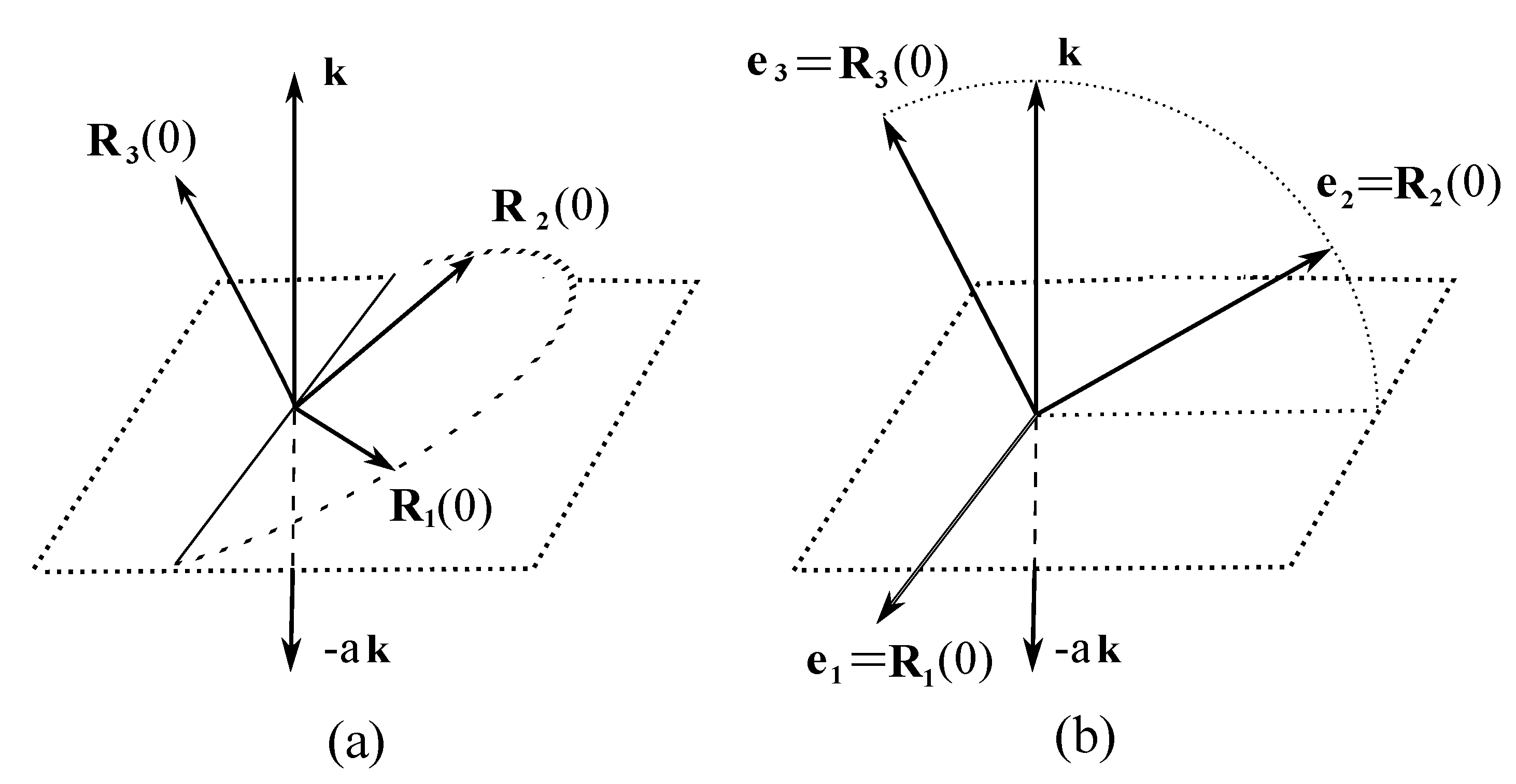
Heavy symmetric body with a fixed point. Let’s consider a rigid body with one fixed point. It is known [5,6,7,8,9] that by placing the origin of the Laboratory system at this point, we arrive at the same equations (1) and (2). Further, let the body is subject to the force of gravity, with the acceleration of gravity equal to

a > 0

and directed opposite to the constant unit vector

k

, see Figure 1a. Then the potential energy of the body’s particle

x_{N} (t)

is

a m_{N} (k, x_{N} (t))

. Summing up the potential energies of the body’s points, we get the total energy

b (k, z (t)) = b (k, R (t) z (0))

. Here

b = a L μ

, L is the distance from the center of mass to the fixed point,

μ

is the total mass of the body and

z (0)

is unit vector in the direction of center of mass at

t = 0

. The potential energy give rise to the torque of gravity in the equations of motion, which read now as follows:

\begin{matrix} I \dot{Ω} = [I Ω, Ω] + b [R^{T} k, z (0)], {\dot{R}}_{i j} = - ϵ_{j k m} Ω_{k} R_{i m} . \end{matrix}

(3)

Let the initial position of the inertia axes

R_{i} (0)

of the body be as shown in Figure 1a. Assuming that the Laboratory axes

e_{i}

have been chosen in the direction of the inertia axes, the matrix I in Eq. (3) acquires the diagonal form. Let us denote components of the vector

k

in this basis as

(k_{1}, k_{2}, k_{3})

.

If our body is a symmetric, that is

I_{1} = I_{2} \neq I_{3}

, our equations can be simplified as follows. Without loss of generality, we can assume that the vector

k

has the following form:

k = (0, k_{2}, k_{3})

. Indeed, the eigenvectors and eigenvalues of the inertia tensor I obey the relations

I R_{i} (0) = I_{i} R_{i} (0)

. With

I_{1} = I_{2}

we have

I R_{1} (0) = I_{2} R_{1} (0)

and

I R_{2} (0) = I_{2} R_{2} (0)

, then any linear combination

α R_{1} (0) + β R_{2} (0)

also represents an eigenvector with eigenvalue

I_{2}

. This means that we are free to choose any two orthogonal axes on the plane

R_{1} (0), R_{2} (0)

as the inertia axes. Hence, in the case

I_{1} = I_{2}

we can rotate the Laboratory axes in the plane

(x^{1}, x^{2})

without breaking the diagonal form of the inertia tensor. Using this freedom, we can assume that

k_{1} = 0

for our problem, see Figure 1(b).

Symmetric (Lagrange) top. Let’s consider the symmetric body,

I_{1} = I_{2} \neq I_{3}

, and assume that its center of mass lies on the axis of inertia

R_{3} (t)

. This body is called the symmetric (or Lagrange) top [9]. This allows further simplify the equations of motion, since by construction

z (0) = {(0, 0, 1)}^{T}

.

With these

k

and

z (0)

, the potential energy acquires the form

b (k_{2} R_{23} + k_{3} R_{33})

. Using these

k

and

z (0)

in Eqs. (3), we get the final form of equations of motion of a heavy symmetric top for the variables

Ω_{i}

and

R_{i j}

. To compare them with those given in textbooks, we rewrite our equations in terms of Euler angles2

\begin{matrix} I_{3} [\dot{ψ} + \dot{φ} cos θ] = m_{ψ} = c o n s t, \end{matrix}

(4)

\begin{matrix} \frac{d}{d t} [I_{2} \dot{φ} {sin}^{2} θ + m_{ψ} cos θ] + b k_{2} sin θ sin φ = 0, \end{matrix}

(5)

\begin{matrix} - I_{2} \ddot{θ} + I_{2} {\dot{φ}}^{2} sin θ cos θ - m_{ψ} sin θ \dot{φ} + b [k_{3} sin θ + k_{2} cos θ cos φ] = 0 . \end{matrix}

(6)

They follow as the conditions of extremum of the following Lagrangian:

\begin{matrix} L = \frac{1}{2} I_{2} [{\dot{θ}}^{2} + {\dot{φ}}^{2} {sin}^{2} θ] + \frac{1}{2} I_{3} {[\dot{ψ} + \dot{φ} cos θ]}^{2} - b [k_{3} cos θ - k_{2} sin θ cos φ] . \end{matrix}

(7)

In the textbooks, equations of motion of the heavy symmetric top follow from a different Lagrangian, the latter does not contain the term proportional to

k_{2}

[9]

\begin{matrix} L_{A} = \frac{1}{2} I_{2} [{\dot{θ}}^{2} + {\dot{φ}}^{2} {sin}^{2} θ] + \frac{1}{2} I_{3} {[\dot{ψ} + \dot{φ} cos θ]}^{2} - b cos θ . \end{matrix}

(8)

This term is discarded on the base of the following reasoning: to simplify the analysis, choose the Laboratory axis

e_{3}

in the direction of the vector

k

... . However, this reasoning does not take into account the presence in the equations of moments of inertia, which have the tensor law of transformation under rotations. Indeed, going back to Eqs. (3), select

e_{3}

in Figure 1(b) in the direction of

k

, and calculate the components of the inertia tensor. Since the axis of inertia

R_{3} (0)

does not coincide with

e_{3}

, we obtain a symmetric matrix instead of a diagonal one, which should now be used in the equations of motion. That is, the attempt to simplify the potential energy leads to a Lagrangian with a complicated expression for the kinetic energy.

Thus, it seems to be necessary to revise the problem of the motion of a heavy symmetric top and correct this drawback.

II. Integrability in quadratures according to Liouville.

Effective Lagrangian with two degrees of freedom. Eq. (4) states that

m_{ψ}

is the integral of motion of the theory (7). Besides, the variable

ψ (t)

does not enter into the remaining equations () and (). So we can look for the effective Lagrangian that implies the equations () and () for the variables

θ

and

φ

. This is as follows:

\begin{matrix} L_{2} = \frac{1}{2} I_{2} [{\dot{θ}}^{2} + {\dot{φ}}^{2} {sin}^{2} θ] + m_{ψ} \dot{φ} cos θ - b [k_{3} cos θ - k_{2} sin θ cos φ], \end{matrix}

(9)

where

m_{ψ}

is considered as a constant. To apply the Liouville’s theorem, we need to rewrite the effective theory in the Hamiltonian formalism. Introducing the conjugate momenta

p_{θ} = \partial L / \partial \dot{θ}

and

p_{φ} = \partial L / \partial \dot{φ}

for the configuration-space variables

θ

and

φ

, we get

\begin{matrix} p_{θ} = I_{2} \dot{θ}, \Rightarrow \dot{θ} = \frac{1}{I_{2}} p_{θ}; p_{φ} = I_{2} \dot{φ} {sin}^{2} θ + m_{ψ} cos θ, \Rightarrow \dot{φ} = \frac{p_{φ} - m_{ψ} cos θ}{I_{2} {sin}^{2} θ} . \end{matrix}

(10)

The Hamiltonian of the system is constructed according the standard rule:

H = p \dot{q} - L (q, \dot{q})

. Its explicit form is as follows:

\begin{matrix} H = \frac{1}{2 I_{2}} [p_{θ}^{2} + {\tilde{p}}_{φ}^{2}] + b U (θ, φ), \end{matrix}

(11)

where it was denoted

\begin{matrix} {\tilde{p}}_{φ} \equiv \frac{p_{φ} - m_{ψ} cos θ}{I_{2} sin θ}, U (θ, φ) \equiv k_{3} cos θ - k_{2} sin θ cos φ . \end{matrix}

(12)

The Hamiltonian equations can be obtained now according the standard rule:

\dot{z} = {z, H}

, where z is any one of the phase-space variables, and the nonvanishing Poisson brackets are

{θ, p_{θ}} = 1

,

{φ, p_{φ}} = 1

.

The effective theory admits two integrals of motion. They are the energy

\begin{matrix} E = \frac{1}{2 I_{2}} [p_{θ}^{2} + {\tilde{p}}_{φ}^{2}] + b U (θ, φ), \end{matrix}

(13)

and the projection of angular momentum on the direction of vector

k

\begin{matrix} m_{φ} = k_{2} p_{θ} sin φ - U_{θ}^{'} {\tilde{p}}_{φ} + m_{ψ} U, w h e r e U_{θ}^{'} \equiv \frac{\partial U}{\partial θ} . \end{matrix}

(14)

The preservation in time of

m_{φ}

can be verified by direct calculation3. The remarcable property of the integrals of motion is that they have vanishing Poisson bracket,

{E, m_{φ}} = 0

, as it can be confirmed by direct calculation. Accoding to the Liouville’s theorem [9,10], this implies that a general solution to the equations of motion can be found in quadratures (that is calculating integrals of some known functions and doing the algebraic operations). Our aim now will be to present the explicit form of the integrals in question.

According to the algorithm used in the proof of Liouville’s theorem [10], we need to resolve Eqs. (13), (14) with respect to

p_{θ}

and

p_{φ}

. Using the identities

\begin{matrix} {(U_{θ}^{'})}^{2} = k_{3}^{2} + k_{2}^{2} {cos}^{2} - U^{2}, {(U_{θ}^{'})}^{2} + k_{2}^{2} {sin}^{2} φ = 1 - U^{2}, U_{θ θ}^{''} = - U, \end{matrix}

(15)

we get the solution

\begin{matrix} p_{φ} = m_{ψ} cos θ + sin θ \frac{- U_{θ}^{'} (m_{φ} - m_{ψ} U) + ϵ k_{2} sin φ \sqrt{2 I_{2} (1 - U^{2}) (E - b U) - {(m_{φ} - m_{ψ} U)}^{2}}}{1 - U^{2}}, \end{matrix}

(16)

\begin{matrix} p_{θ} = \frac{k_{2} sin φ (m_{φ} - m_{ψ} U) + ϵ U_{θ}^{'} \sqrt{2 I_{2} (1 - U^{2}) (E - b U) - {(m_{φ} - m_{ψ} U)}^{2}}}{1 - U^{2}}, \end{matrix}

(17)

where

ϵ = \pm 1

. Next we need to integrate these functions along any curve connecting the origin of configuration space with a point

(θ, φ)

. Taking the curve to be a pair of intervals,

(0, 0) \to (θ, 0) \to (θ, φ)

, we obtain the following function

\begin{matrix} Φ (θ, φ, E, m_{φ}) = \int_{0}^{θ} p_{θ} (θ^{'}, 0, E, p_{φ}) d θ^{'} + \int_{0}^{φ} p_{φ} (θ, φ^{'}, E, p_{φ}) d φ^{'} . \end{matrix}

(18)

Then the general solution to the equations of motion of the theory (9) is obtained resolving Eqs. (16) together with the equations

c_{1} = - t + \partial Φ / \partial E

,

c_{2} = \partial Φ / \partial m_{φ}

with respect to the phase-space variables

θ, p_{θ}, φ, p_{φ}

. Using (18), the last two equations read as follows:

\begin{matrix} c_{1} = - t + \int_{0}^{θ} \partial_{E} p_{θ} (θ^{'}, 0, E, m_{φ}) d θ^{'} + \int_{0}^{φ} \partial_{E} p_{φ} (θ, φ^{'}, E, m_{φ}) d φ^{'}, \end{matrix}

(19)

\begin{matrix} c_{2} = \int_{0}^{θ} \partial_{m_{φ}} p_{θ} (θ^{'}, 0, E, m_{φ}) d θ^{'} + \int_{0}^{φ} \partial_{m_{φ}} p_{φ} (θ, φ^{'}, E, m_{φ}) d φ^{'} . \end{matrix}

(20)

Calculating the partial derivatives indicated in these integrals, we get

\begin{matrix} \int_{0}^{θ} \partial_{E} p_{θ} (θ^{'}, 0) d θ^{'} = ϵ I_{2} \int \frac{d U}{\sqrt{2 I_{2} (1 - U^{2}) (E - b U) - {(m_{φ} - m_{ψ} U)}^{2}}}, \end{matrix}

(21)

\begin{matrix} \int_{0}^{θ} \partial_{m_{φ}} p_{θ} (θ^{'}, 0) d θ^{'} = - ϵ \int \frac{(m_{φ} - m_{ψ} U) d U}{(1 - U^{2}) \sqrt{2 I_{2} (1 - U^{2}) (E - b U) - {(m_{φ} - m_{ψ} U)}^{2}}}, \end{matrix}

(22)

\begin{matrix} \int_{0}^{φ} \partial_{E} p_{φ} (θ, φ^{'}) d φ^{'} = - ϵ I_{2} k_{2} sin θ \int \frac{d (cos φ^{'})}{\sqrt{2 I_{2} (1 - U^{2}) (E - b U) - {(m_{φ} - m_{ψ} U)}^{2}}}, \end{matrix}

(23)

\begin{matrix} \int_{0}^{φ} \partial_{m_{φ}} p_{φ} (θ, φ^{'}) d φ^{'} = - sin θ \int_{0}^{φ} \frac{U_{θ}^{'} d φ^{'}}{1 - U^{2}} + ϵ k_{2} sin θ \int \frac{(m_{φ} - m_{ψ} U) d (cos φ^{'})}{(1 - U^{2}) \sqrt{2 I_{2} (1 - U^{2}) (E - b U) - {(m_{φ} - m_{ψ} U)}^{2}}} . \end{matrix}

(24)

These are elliptic integrals over the indicated integration variables.

III. Conclusion.

When formulating and solving the equations of motion of a rigid body with the inertia tensor chosen in the diagonal form, one should keep in mind the tensor law of transformation of the moments of inertia

I_{1}, I_{2}, I_{3}

under rotations. We observed that for the symmetric top this leads to the potential energy that depends on the Euler angles

φ

and

θ

. The potential energy (7) is different from that assumed in textbooks (8). So we revised the problem of the motion of a heavy symmetric top and corrected this drawback. We confirmed that the improved equations of motion () and () are integrable according to Liouville, and reduced the problem to the elliptic integrals (21)-(24).

In the absence of analytic solution, we could look for one-dimensional effective Lagrangian, say

L (θ, \dot{θ})

, and try to analyze qualitatively the corresponding effective potential [6,9]. To find it, it is necessary to solve with respect to

cos φ

and

\dot{φ}

the equations, which represent the integrals of motion E and

m_{φ}

. However, this implies the search for the roots of a polinomial of degree 6.

Acknowledgments

The work has been supported by the Brazilian foundation CNPq (Conselho Nacional de Desenvolvimento Científico e Tecnológico - Brasil).

Notes

1	Failure to take this circumstance into account leads to a lot of confusion, see [11].
2	See Appendix 1 in [1] for the details.
3	In terms of the variables $Ω_{i}$ and $R_{i j}$ the integral of motion $m_{φ}$ reads as follows: $m_{φ} = (k, R I Ω) \equiv (k, m)$ , where $m = R I Ω$ is the angular momentum of the top. Its preservation in time ${\dot{m}}_{φ} = 0$ follows also from Eqs. (3).

References

A. A. Deriglazov, Lagrangian and Hamiltonian formulations of asymmetric rigid body, considered as a constrained system, arXiv:2301.10741.
A. A. Deriglazov, Geodesic motion on the symplectic leaf of SO(3) with distorted e(3) algebra and Liouville integrability of a free rigid body, Eur. Phys. J. C (2023) 83:265; arXiv:2302.04828.
A. A. Deriglazov, Poincaré-Chetaev equations in the Dirac’s formalism of constrained systems, arXiv:2302.12423.
A. A. Deriglazov, General solution to the Euler-Poisson equations of a free Lagrange top directly for the rotation matrix, arXiv:2303.02431.
E. T. Whittaker, A treatise on the analytical dynamics of particles and rigid bodies, (Cambridge: at the University press, 1917).
W. D. MacMillan, Dynamics of rigid bodies, (Dover Publications Inc., New-York, 1936).
E. Leimanis, The general problem of the motion of coupled rigid bodies about a fixed point, (Springer-Verlag, 1965).
H. Goldstein, C. Poole and J. Safko, Classical mechanics, Third edition, (Addison Wesley, 2000).
V. I. Arnold, Mathematical methods of classical mechanics, 2nd edn. (Springer, New York, NY, 1989).
A. V. Bolsinov and A. T. Fomenko, Integrable Hamiltonian systems, (Charman and Hall/CRC, 2004).
A. A. Deriglazov, Comment on the Letter "Geometric Origin of the Tennis Racket Effect” by P. Mardesic, et al, Phys. Rev. Lett. 125, 064301 (2020), arXiv:2302.04190.

Figure 1. (a) - Initial position of a heavy top with orthogonal inertia axes

R_{1} (0), R_{2} (0), R_{3} (0)

. (b) - Due to the freedom in the choice of

R_{1} (0)

and

R_{2} (0)

, the vector

k

can be taken in the form

k = (0, k_{2}, k_{3}) .

Figure 1. (a) - Initial position of a heavy top with orthogonal inertia axes

R_{1} (0), R_{2} (0), R_{3} (0)

. (b) - Due to the freedom in the choice of

R_{1} (0)

and

R_{2} (0)

, the vector

k

can be taken in the form

k = (0, k_{2}, k_{3}) .

Disclaimer/Publisher’s Note: The statements, opinions and data contained in all publications are solely those of the individual author(s) and contributor(s) and not of MDPI and/or the editor(s). MDPI and/or the editor(s) disclaim responsibility for any injury to people or property resulting from any ideas, methods, instructions or products referred to in the content.

© 2023 by the authors. Licensee MDPI, Basel, Switzerland. This article is an open access article distributed under the terms and conditions of the Creative Commons Attribution (CC BY) license (http://creativecommons.org/licenses/by/4.0/).

Copyright: This open access article is published under a Creative Commons CC BY 4.0 license, which permit the free download, distribution, and reuse, provided that the author and preprint are cited in any reuse.

Has the Problem of the Motion of a Heavy Symmetric Top Been Solved in Quadratures?

Abstract

Keywords:

Subject:

I. Introduction

II. Integrability in quadratures according to Liouville.

III. Conclusion.

Acknowledgments

Notes

References

MDPI Initiatives

Important Links

Subscribe