
Submitted:
03 June 2023
Posted:
05 June 2023
You are already at the latest version
Abstract
For a system that turns out to be inactive in time t, the past entropy is considered as an
uncertainty measure for the past lifetime distribution. In this study, we consider a coherent system
that includes n components and has the property that all the components of the system have failed at
time t. To assess the predictability of the coherent system’s lifetime, we use the system’s signature
to determine the Rényi entropy of its past lifetime. We study several analytical results, including
expressions, bounds, and order properties for this measure.
Keywords:
coherent system
; past entropy
; Shannon differential entropy
; system signature
1. Introduction
An accurate quantification of uncertainty of system lifetime is an important task for engineers engaged in survival analysis. The importance of reducing uncertainty and increasing system lifetime is widely recognized, with longer lifetimes and lower uncertainties being key indicators of higher system reliability (see, e.g., [1]). The problem of extending the life cycle of engineering systems is extremely important and has serious practical applications. To this end, we use the concept of Rényi entropy, denoted , which measures the uncertainty associated with a nonnegative continuous random variable (rv) X with a probability density function (pdf) defined as the Rényi entropy of order , which is as follows
where “log" stands as the natural logarithm. In general, uncertainty in the lifetime of a device or organism can be described by a non-negative rv X with a pdf . This is distinct from uncertainty associated with a probability p measured by its Shannon entropy . The notion of uncertainty in the context of a distribution, which is well defined for a discrete distribution, should be used with caution when dealing with a continuous distribution, and even more so when choosing the Rényi entropy. In the continuous case, it is important to note that unlike the discrete case, the Rényi entropy need not be positive. A probability distribution is typically used to quantify uncertainty and depends on information about the probability that the uncertain quantity has a single, true value. A distribution of the frequencies of numerous instances of the variable, obtained from observed data, is used to quantify variation. In our case, the variable is the random lifetime of the device, and the uncertainty is a function of event probabilities. Events, in the context of rvs, are those where a random lifetime has certain numerical values.
Rényi entropy has many applications in measuring uncertainty in dynamical systems and has also proved to be a useful criterion for optimization problems (see e.g., Erdogmus and Principe [2], Lake [3], Bashkirov [4] Henríquez et al. [5]), Guo et al. [6], Ampilova and Soloviev [7], Koltcov [8] and Wang et al. [9]. Shannon’s differential entropy (Shannon [10]), a fundamental concept in information theory, can be derived as follows:
By consideration of the lifetime a fresh system has, denoted by X, the Rényi entropy is a useful measure of uncertainty. However, in certain scenarios, actors may know the current age of the system. For example, they know that the system has been in operation for a certain period of time t and want to measure the uncertainty induced by the remaining lifetime of the system, denoted by . In such cases, Rényi entropy is no longer an appropriate measure of uncertainty. To address this problem, we introduce the residual Rényi entropy, which is specifically designed to measure the uncertainty associated with the remaining lifetime of a system. The residual Rényi entropy is (see [11])
for all where denotes the survival function of the rv The concept of provides a fascinating aspect of lifetime units in reliability engineering as the behaviour of its fluctuations with respect to t (the current age of an item with original lifetime X) may be helpful to create models. This area of research has attracted the attention of researchers in various fields of science and engineering. This entropy measure is a generalization of the classical Shannon entropy, and it has been shown to have numerous valuable properties and applications in different contexts. In this area, Asadi et al. [12], Gupta and Nanda [13], Nanda and Paul [14], Mesfioui et al. [15], and many other researchers have studied the properties and applications of .
Uncertainty is a pervasive feature of a given (specific) parameter in real systems, such as their random lifetime, and its effects are felt not only in the future but also in the past. Even if there are facts in the past that we are not aware of, uncertainty remains. There are many real situations in nature, in society, in history, in geology, in other branches of science, and even in medicine, where there is no information about the exact timing of some past events. For example, the exact time when a disease began in a person’s body. This gives rise to a complementary notion of entropy, which captures the uncertainty of past events and is distinct from residual entropy, which describes uncertainty about future events. For another example, consider a system that is observed only at certain inspection times. If the system is inspected for the first time at time t and is in a failed state, the uncertainty relates to the past, more specifically to the time of failure within the interval . Moreover: When an aircraft is discovered in a non-functional state, it is critical to quantify the degree of uncertainty associated with this situation, which is in the past. The uncertainty is in determining the exact point in the aircraft’s operational history that led to its current condition. Therefore, it is appropriate to introduce a complementary notion of uncertainty that refers to past events rather than future events and is distinct from residual entropy. Let denote an rv with the conditional distribution of Z under the assumption that Z lies in where A is a subset of such that . Suppose that X is the random lifetime of a fresh system that has a cumulative distribution function (cdf) F, and suppose that an inspection at time t finds that the system is inactive. Then for all , which is known as the inactivity time of the system and measures the time elapsed since the time when the failure of the system occurred (cf. Kayid and Ahmad [16]). The rv is also called the past lifetime. The uncertainty in distribution of , is equivalent to the uncertainty in the in the rv . The study of past entropy, which deals with the entropy properties of the distribution of past lifetimes, and its statistical applications have received considerable attention in the literature, as evidenced by works such as Di Crescenzo and Longobardi [17], Nair and Sunoj [18], and Nair and Sunoj [19]. Li and Zhang [20] studied monotonic properties of entropy in order statistics, record values, and weighted distributions in terms of Rényi entropy. Gupta et al. [21] have made significant contributions to the field by studying the properties and applications of past entropy in the context of order statistics. In particular, they have studied the residual and past entropies of order statistics and made stochastic comparisons between them. In general, the informational properties of the residual lifetime distribution are not related to the informational aspects of the past lifetime distribution, at least not for lifetime distributions, which is the case in this work. For further illustrative descriptions on this issue we refer the reader to Ahmad et al. [22]. Therefore, the study of uncertainty in the past life distribution was considered as a new problem compared to the uncertainty properties of the residual life distribution.
On the other hand, coherent systems are well-known in reliability engineering as a large class of such systems and as typical systems in practice (see, e.g., Barlow and Proschan [23] for the formal definition and initial properties of such systems). An example is the k-out-of-n system, which denotes a structure with n components, of which at least k components must be active for the whole system to work. This structure is one of the most important special cases of coherent systems, which has many applications. For example, an airplane with three engines, where at least two engines must be active for it to continue flying smoothly. The out-of-n structure, referred to in the literature as fail-safe systems, has many applications in the real world. A fail-safe system is a special design feature that, when a failure occurs, reacts in such a way that no damage is done to the system itself. The brake system on a train is an excellent example of a fail-safe system, where the brakes are held in the off position by air pressure. If a brake line ruptures or a car is cut off, the air pressure is lost; in this case, the brakes are applied by a local air reservoir. Consider a coherent system that turns out to be inactive at time t, when all components of the system are also inactive. The time t is the first time at which the coherent system is found to be inactive. The predictability of the exact time at which the system fails depends largely on the uncertainty properties of the past lifetime distributions. The goal of this work is to quantify the uncertainty about the exact time of failure of the coherent system that is inactive at time t, and furthermore, the uncertainty about the exact time of failure of a particular component of this inactive system. To this end, we will utilize the Rényi entropy of past life distribution. Throughout the manuscript, we will not use the words “increasing” and “decreasing” in the strict sense.
In this paper, we present a comprehensive study of Rényi entropy for the distribution of past lifetimes, providing a generalized version of the Equation (3). By allowing different averaging of the conditional probabilities by the parameter , our proposed measure allows for a nuanced comparison of the shapes of different distributions of past lifetimes. The present results demonstrate the potential of this measure to uncover new insights into the mechanisms underlying these distributions. Furthermore, we assume a coherent system of n components, characterized by the property that all components of the system have failed at time We use the system signature method to calculate the Rényi entropy of the past lifetime of a coherent system.
2. Results on the Past Rényi Entropy
Let us consider an rv X representing the lifetime of a system with the pdf and the cdf . Recall that the pdf of is given by where and for and . The rvs and are called right-truncated rvs associated with X and respectively. In this context, the past Rényi entropy at time t of X is defined as (see e.g., [13])
for all Note that . Suppose that at time t it is determined that a lifetime unit has failed. Then measures the uncertainty about its past lifetime, i.e., about . The role of past Rényi entropy in comparing random lifetimes is illustrated by the following example. This highlights the importance of our proposed measure in detecting subtle differences in the shapes of different distributions of past lifetimes and underscores its potential to shed light on the mechanisms underlying these phenomena.
Example 1.
Let us consider two components in a system having random lifetimes X and Y with pdfs
respectively. The Rényi entropy of both X and Y are elegantly captured by the expression:
This result implies that the expected uncertainty regarding the predictability of the outcomes of X and Y in terms of Rényi entropy is identical for f and g. In the case where both components failed at time during the inspection, the past Rényi entropy can be used to measure the uncertainty around the respective failure time points, in spirit of the Equation (4) as follows:
It can be shown that , for all i.e., the expected uncertainty related to the predictability of the failure time of the first component with original lifetime X as long as , is greater than that of the second component with original lifetime Y provided that , even if .
As mentioned before in Section 1, an interesting observation is that the statement in the Equation (4) can be interpreted as the Rényi entropy of the inactivity time This alternative identification sheds new light on the underlying dynamics. From (4) we also obtain the following expressions for the past Rényi entropy:
where denotes the reversed hazard rate of X and has the pdf as
for all , so that for all . The following definition which can be found in Shaked and Shanthikumar [24] is used throughout the paper.
Definition 1.
Suppose that X and Y are two general rvs with arbitrary supports with density functions f and g and reversed hazard rate functions and respectively. Then,
- (i)
- We say X is smaller than Y in the reversed hazard rate order (denoted by ) whenever for all a, or equivalently if, is increasing in
- (ii)
- X is said to have decreasing [resp. increasing] reversed hazard rate property (denoted as DRHR [resp. IRHR]) whenever is a decreasing [resp. increasing] function in a.
- (iii)
- We say X is smaller than Y in the dispersion order (denoted by ) whenever for all
Our analysis sheds new light on the behavior of past Rényi entropy in the presence of decreasing reversed hazard rate (DRHR) property, contributing to our understanding of this important class of stochastic processes.
Theorem 1.
If X is DRHR, then is increasing in t.
Proof .
The result of Theorem 1 shows that the DRHR property of a component lifetime translates to the increasing property of past Rényi entropy for the component lifetime as a function of time. Thus, an interesting conclusion is that when we first find that a component with a random lifetime exhibiting the DRHR property has failed, the uncertainty about the exact time of failure (with respect to the past Rényi entropy) of the component increases accordingly. The following theorem refers to the ordering of the rvs according to the Rényi entropy of the right-truncated distributions and the ordering of the rvs based on the basis of the reversed hazard rates order.
Theorem 2.
Let X and Y be two continuous rvs having cdfs F and G with pdfs f and and reversed hazard rate functions and respectively. If and either X or Y has IRHR property, then, for all , we have .
Proof.
Notice that and as two right-truncated rvs, have pdfs and respectively. The condition that implies that for all
For every , the inequality
then holds which further implies that , where and have the cdfs and , respectively. Now, let us assume that X has IRHR property. For we obtain the following result
where the former inequality follows from the definition of the usual stochastic order and the fact that for all increasing functions and in particular, for which is an increasing function of x as X is IRHR and also since . The latter inequality above is also satisfied because of . For we can easily check that
For all we finally get
and this gives by recalling (6). A similar conclusion can be drawn if we assume instead that the rv Y possesses the IRHR property. □
According to Theorem 2, between two rvs, at least one of which has the IRHR property, the one with a larger reversed hazard rate leads to smaller uncertainty in Rényi entropy of the right truncated distribution. Therefore, the rv, which is stochastically smaller, is expected to be less predictable.
In the next theorem, we give a bound for in terms of the reversed hazard rate function.
Theorem 3.
Assume that If X is DRHR, then for all it holds that
Proof.
If X is DRHR, then is decreasing in and so recalling (6) for all we have
and this completes the proof. □
3. Results on the Past Lifetime of Coherent Systems
This section presents the application of the system signature approach to find a definition for the past-life entropy of a coherent system with arbitrary structure. It is assumed that all components of the system have failed at a given time A coherent system is defined as one that satisfies two conditions: First, it contains no irrelevant components, and second, its structure function is monotonic. An n-dimensional vector whose ith element is given by is the signature of such a system (see [25]). Consider a coherent system with independent and identically distributed (i.i.d.) component lifetimes , and a known signature vector . If stands for the past lifetime of the coherent system under the condition that at time all components of the system have failed, then from the results of Khaledi and Kochar [26] the survival function of can be expressed as
where
denotes the past-life survival function of an i-out-of-n system under the condition that all components have failed at time t. From (9) it follows that
where
such that is the complete gamma function and is the time that has passed from the failure of the component with lifetime in the system given that the system has failed at or before time It is worth mentioning, by (9), that denotes the ith order statistics consisting of n i.i.d. components with the cdf Hereafter, we provide an expression for the entropy of To this aim, let us keep in mind that The probability integral transformation as a crucial reformulation plays an important role in our aim. It is evidently seen that has the beta distribution with parameters i and with the following pdf
for all In the forthcoming theorem, we provide an expression for the Rényi entropy of by using the earlier mentioned transforms.
Theorem 4.
Let stand for the past lifetime of the coherent system under the condition that, at time all components of the system have failed. The Rényi entropy of can be expressed as follows:
where V is the lifetime of the coherent system with the pdf and is the quantile function of for all
Proof.
The identity at the last line above is acquired by substituting , which ends the proof. □
If all components have failed at time t, then measures the expected uncertainty contained in the conditional density of given about the predictability of the past lifetime of the system. In the special case, if we consider an i-out-of-n system with the system signature , then Equation (13) reduces to
where has the beta distribution with parameters and and
so that stands for the beta function. In the special case when t goes to infinity, (14) coincides with the results of Abbasnejad and Arghami [27].
The next theorem immediately follows from Theorem 4 in terms of the property that the reversed hazard rate of X i.e., is decreasing.
Theorem 5.
If X is DRHR, then is increasing in t.
Proof.
Remark 1.
The result of Theorem 5 in turn shows that when the component lifetimes in a coherent system satisfy the DRHR property, the past Rényi entropy increases when all components of the coherent system are inactive thus decreasing predictability and making it very difficult to determine the exact time of failure in the past.
The next example is given to apply Theorems 4 and 5.
Example 2.
- (i)
- Let X follow the uniform distribution in From (13), we immediately obtainIt reveals that the Rényi entropy of the rv is a decreasing function of time t. This observation is consistent with previous results on the behavior of Rényi entropy for certain classes of rvs. In particular, the uniform distribution is known to possess the DRHR property, which implies that the Rényi entropy of should be an increasing function of time t, in line with Theorem 5.
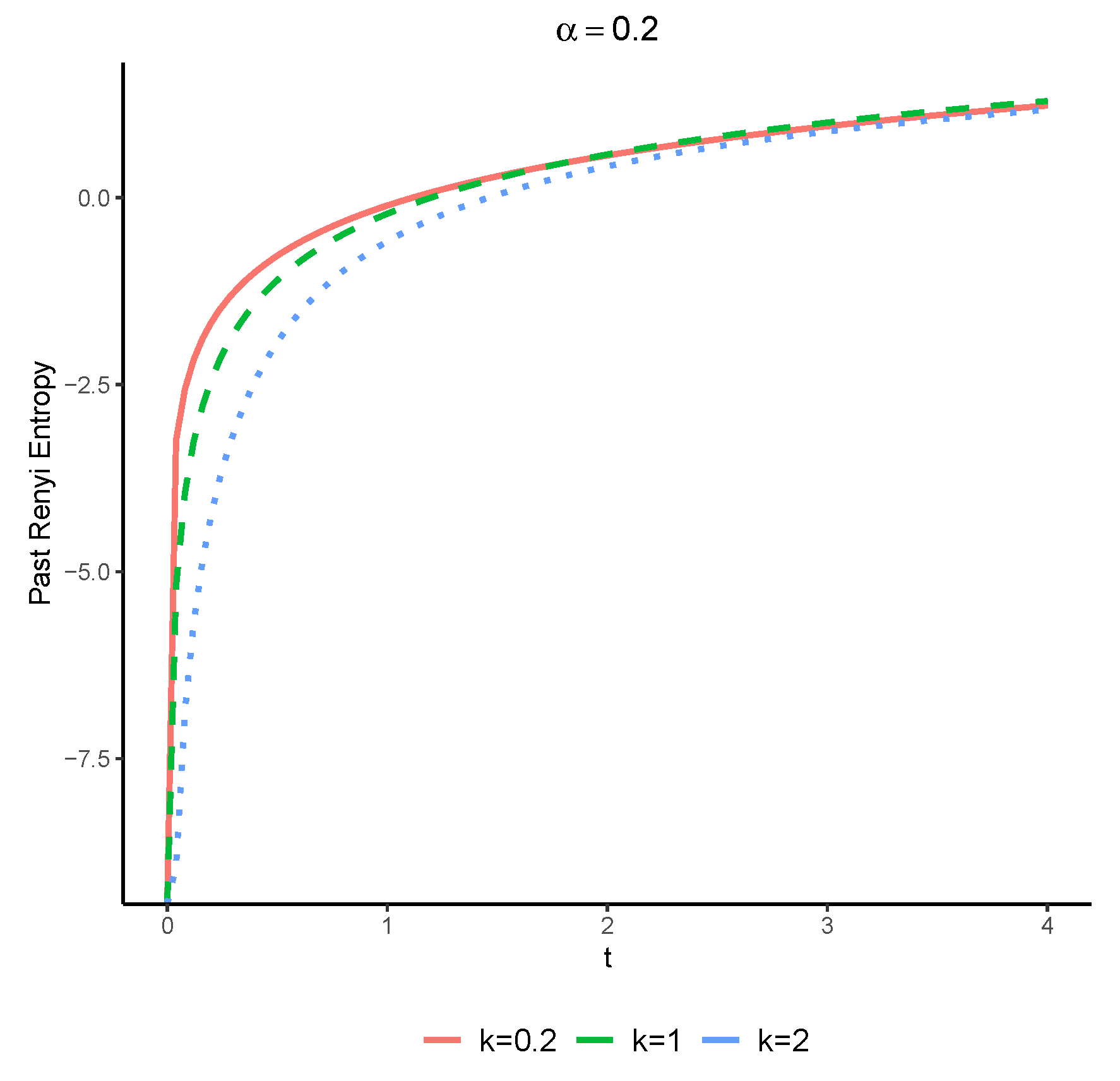
- (b)
- Consider an rv X with the cdf given byWith some algebraic manipulation, we arrive at the following expression:The numerical results, which are presented in Figure 2, showcase the increasing nature of the Rényi entropy of as a function of time t, for and various values of k (in this case, the past Rényi entropy for is not defined). This observation is in line with Theorem 5, which predicts the monotonicity properties of the Rényi entropy in the case of DRHR rvs.
The above example sheds light on the complicated relationship between the Rényi entropy of an rv and time t (the time of inspection) where the failure of the device is realized, and highlights the importance of considering the DRHR property when analyzing such systems. Thus, our results suggest that the DRHR property of X plays a crucial role in shaping the temporal behavior of the Rényi entropy of , which could have far-reaching implications for various applications, including the analysis of complex systems and the development of efficient data compression techniques.
It is possible to lower the computing cost for determining the signatures of all coherent systems of a certain size by around half thanks to the widely used notion of a system’s dual in reliability and industry. A duality link between a system’s signature and that of its dual has been proposed by Kochar et al. [28]. If signifies the signature of a coherent system with lifetime T, then the signature by which its dual system with lifetime is recognized, is given by . In the following theorem, we apply the duality property to simplify the calculation of the past Rényi entropy for coherent systems.
Theorem 6.
Let be the lifetime of a coherent system with signature consisting of n i.i.d. components. If satisfies for all and then for all and all
Proof.
In the following, a direct conclusion is drawn from Theorem 6 for the case that an i-out-of-n-system is the designated coherent system.
Corollary 1.
Let be the lifetime of an i-out-of-n system consisting of n i.i.d. components. If satisfies for all and then for all n and if n is even and if n is odd.
4. Bounds for the Past Rényi Entropy of Coherent Systems
For complex systems or uncertain distributions of component lifetimes, accurately calculating the past Rényi entropy of a coherent system can be a daunting task. This scenario is not uncommon in practice, and thus there is a growing need for effective approximations of the system behavior. One promising approach is to use previous Rényi entropy bounds, which have been shown to accurately approximate the lifetime of coherent systems under such circumstances.
Toomaj and Doostparast [29,30] pioneered the development of such barriers for a new system, while more recently Toomaj et al. [31] has extended this work by deriving bounds on the entropy of a coherent system when all its components are working; see also Mesfioui et al. [15]. In the following theorem, we introduce new bounds on the past Rényi entropy of the coherent system’s lifetime, expressed in terms of the past Rényi entropy of the higher-order distribution . By incorporating these bounds into our analysis, we can achieve a more accurate and efficient characterization of complex systems, even in the face of limited information about component lifetimes.
Theorem 7.
Assume a coherent system with the past lifetime consisting of n i.i.d. component lifetimes having the common cdf F with the signature . Then, we have
for where and
Proof.
The beta distribution with parameters and i is a well-known distribution where its mode, denoted by , can be conveniently expressed as . This result allows us to obtain the following expression:
Thus, for we have
The last equality is obtained from (4) which the desired result follows. □
The lower and upper bounds shown in Equation (17) are a valuable tool for analyzing systems with a large number of components or complex configurations. However, in situations where these bounds are not applicable, we can resort to the Rényi information measure and mathematical concepts to derive a more general lower bound. This approach leverages the power of the Rényi information measure and mathematical ideas to provide new insights into the behavior of complex systems, which will be presented in the next theorem.
Theorem 8.
In the setting of Theorem 7,
where for all
Proof.
The Jensen’s inequality for the function (it is concave (convex) for ) yields
and hence we get
The above inequality is obtained by the linearity property of integration. Since , by multiplying both side (20) in , we get the desired result. □
It is noteworthy that the equality condition in (19) holds true for i-out-of-n systems, where the failure probability is zero for , and one for . In this case, the conditional entropy of the system is equal to the conditional entropy of the ith component . When the lower bounds for in both parts of Theorems 7 and 8 can be computed, one may use the maximum of the two lower bounds.
Example 3.
Let represent the past lifetime of a coherent system with the signature consisting of i.i.d. component lifetimes according to standard exponential distribution with cdf It is easily seen that
Moreover, we can get Thus, by Theorem 7, the Rényi entropy of is bounded for as follows:
It is easily seen that
for all So, the lower bound given in (19) can be obtained as follows:
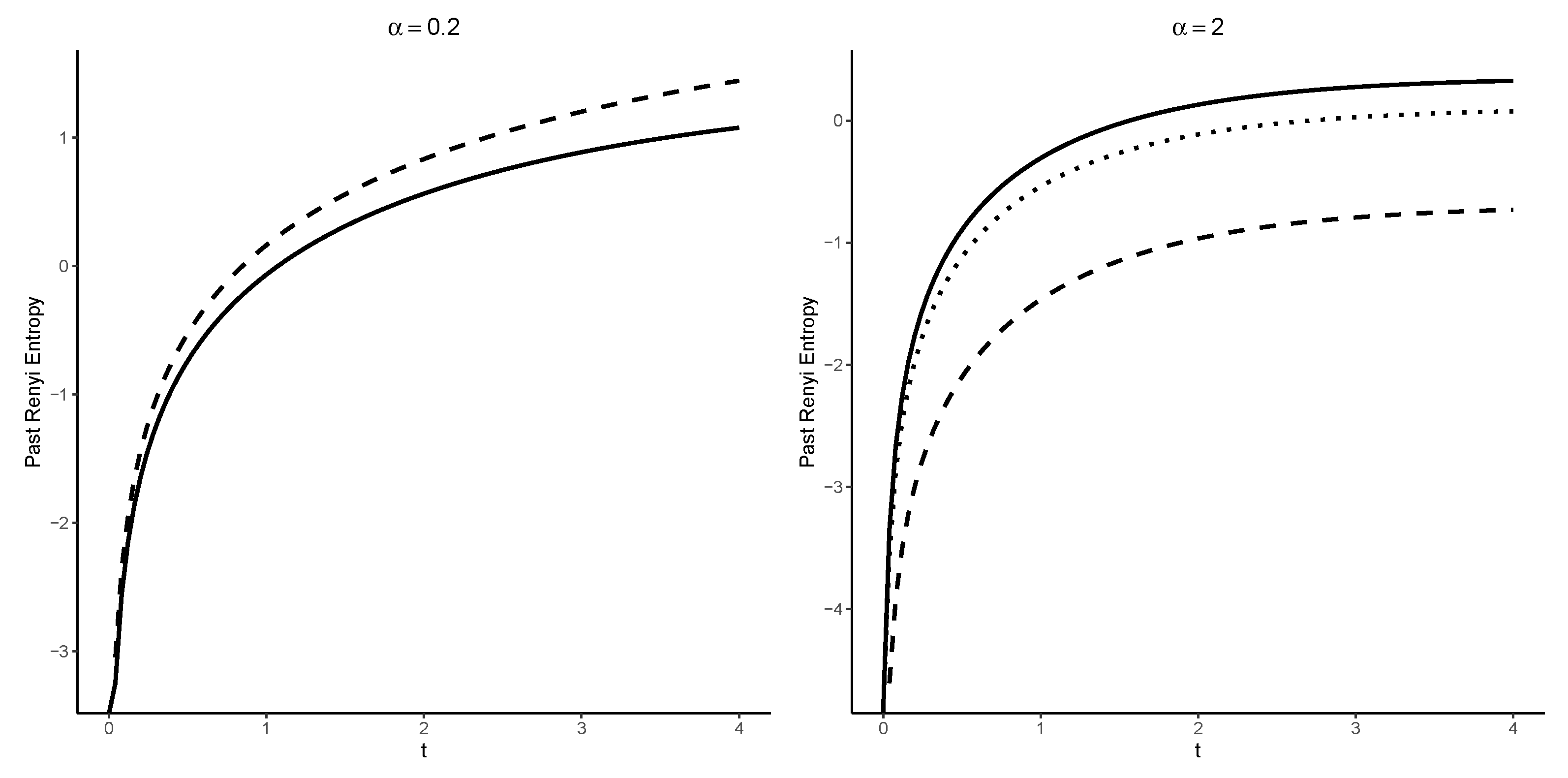
for all Figure 3 depicts the time evolution of the Rényi entropy for the standard exponential distribution. The solid line represents the exact value of , while the dashed and dotted lines correspond to the bounds derived from Equations (21) and (22), respectively. The figure provides a clear visualization of the behavior of the past Rényi entropy over time and highlights the remarkable agreement between the exact value and the bounds. Notably, for , the lower bound from (22) (dotted line) surpasses the lower bound from (21).
5. Concluding Remarks
In recent years, the assessment of predictability has become very important when considering the lifetime of engineering systems. Quantification of uncertainty is a crucial criterion for measuring the degree of predictability in such systems. The Rényi entropy has proven to be an attractive measure for quantifying the uncertainty associated with the lifetime of systems. In this work, we have presented an expression for the Rényi entropy of the lifetime of a system, under the condition that all system components have failed at time t. This situation may arise in practice because the time at which we normally observe a system and detect the failure of a system is quite late, so all components of the coherent system have also failed at that time. Moreover, we investigate the various properties of this proposed measure, including the determination of boundaries and partial orders between the random time points that have elapsed since the failure of two coherent systems, based on their Rényi entropy uncertainties using the concept of system signature. Our approach provides an effective method for assessing the predictability of system lifetimes and is useful for engineering applications. We demonstrate the effectiveness of our proposed measure using several application examples. It is worth noting that the results of this paper can be used to study the predictability of engineering systems and its relevance to current research. The results presented provide compelling evidence for the value of Rényi entropy in engineering reliability analysis and highlight its potential for future research in this area.
Author Contributions
Conceptualization, M.K.; methodology, M.K.; software, M.S.; validation, M.K.; formal analysis, M.K.; investigation, M.S.; resources, M.S.; writing—original draft preparation, M.K.; writing—review and editing, M.S.; visualization, M.S.; supervision, M.S.; project administration, M.S.; funding acquisition, M.S. All authors have read and agreed to the published version of the manuscript.
Funding
Researchers Supporting Project number (RSP2023R464), King Saud University, Riyadh, Saudi Arabia.
Institutional Review Board Statement
Not applicable.
Informed Consent Statement
Not applicable.
Data Availability Statement
Not applicable.
Acknowledgments
The authors are grateful to two anonymous reviewers for their constructive comments and suggestions. The authors acknowledge financial support from the Researchers Supporting Project number (RSP2023R464), King Saud University, Riyadh, Saudi Arabia.
Conflicts of Interest
The authors declare no conflict of interest.
References
- Ebrahimi, N.; Pellerey, F. New partial ordering of survival functions based on the notion of uncertainty. Journal of applied probability 1995, 32, 202–211. [Google Scholar] [CrossRef]
- Erdogmus, D.; Principe, J.C. An error-entropy minimization algorithm for supervised training of nonlinear adaptive systems. IEEE Transactions on Signal Processing 2002, 50, 1780–1786. [Google Scholar] [CrossRef]
- Lake, D.E. Renyi entropy measures of heart rate Gaussianity. IEEE Transactions on Biomedical Engineering 2005, 53, 21–27. [Google Scholar] [CrossRef] [PubMed]
- Bashkirov, A.G. Renyi entropy as a statistical entropy for complex systems. Theoretical and Mathematical Physics 2006, 149, 1559–1573. [Google Scholar] [CrossRef]
- Henríquez, P.; Alonso, J.B.; Ferrer, M.A.; Travieso, C.M.; Godino-Llorente, J.I.; Díaz-de María, F. Characterization of healthy and pathological voice through measures based on nonlinear dynamics. IEEE transactions on audio, speech, and language processing 2009, 17, 1186–1195. [Google Scholar] [CrossRef]
- Guo, L.; Yin, L.; Wang, H.; Chai, T. Entropy optimization filtering for fault isolation of nonlinear non-Gaussian stochastic systems. IEEE Transactions on Automatic Control 2009, 54, 804–810. [Google Scholar]
- Ampilova, N.; Soloviev, I. Entropies in investigation of dynamical systems and their application to digital image analysis. Journal of Measurements in Engineering 2018, 6, 107–118. [Google Scholar] [CrossRef]
- Koltcov, S. Application of Rényi and Tsallis entropies to topic modeling optimization. Physica A: Statistical Mechanics and its Applications 2018, 512, 1192–1204. [Google Scholar] [CrossRef]
- Wang, Z.; Pang, C.K.; Ng, T.S. Data-driven scheduling optimization under uncertainty using Renyi entropy and skewness criterion. Computers & Industrial Engineering 2018, 126, 410–420. [Google Scholar]
- Shannon, C.E. A mathematical theory of communication. The Bell system technical journal 1948, 27, 379–423. [Google Scholar] [CrossRef]
- Abraham, B.; Sankaran, P. Renyi’s entropy for residual lifetime distribution. Statistical Papers 2006, 47, 17–29. [Google Scholar] [CrossRef]
- Asadi, M.; Ebrahimi, N.; Soofi, E.S. Dynamic generalized information measures. Statistics & probability letters 2005, 71, 85–98. [Google Scholar]
- Gupta, R.; Nanda, A. α-and β-entropies and relative entropies of distributions. Journal of Statistical Theory and Applications 2002, 1, 177–190. [Google Scholar]
- Nanda, A.K.; Paul, P. Some results on generalized residual entropy. Information Sciences 2006, 176, 27–47. [Google Scholar] [CrossRef]
- Mesfioui, M.; Kayid, M.; Shrahili, M. Renyi Entropy of the Residual Lifetime of a Reliability System at the System Level. Axioms 2023, 12, 320. [Google Scholar] [CrossRef]
- Kayid, M.; Ahmad, I. On the mean inactivity time ordering with reliability applications. Probability in the Engineering and Informational Sciences 2004, 18, 395–409. [Google Scholar] [CrossRef]
- Di Crescenzo, A.; Longobardi, M. Entropy-based measure of uncertainty in past lifetime distributions. Journal of Applied probability 2002, 39, 434–440. [Google Scholar] [CrossRef]
- Nair, N.U.; Sunoj, S. Some aspects of reversed hazard rate and past entropy. Communications in Statistics-Theory and Methods 2021, 32, 2106–2116. [Google Scholar] [CrossRef]
- Nair, N.U.; Sunoj, S. Some New Results on Renyi Entropy and Its Relative Measure. Calcutta Statistical Association Bulletin 2022, 74, 97–116. [Google Scholar] [CrossRef]
- Li, X.; Zhang, S. Some new results on Rényi entropy of residual life and inactivity time. Probability in the Engineering and Informational Sciences 2011, 25, 237–250. [Google Scholar] [CrossRef]
- Gupta, R.C.; Taneja, H.; Thapliyal, R. Stochastic comparisons of residual entropy of order statistics and some characterization results. Journal of Statistical Theory and Applications 2014, 13, 27–37. [Google Scholar] [CrossRef]
- Ahmad, I.A.; Kayid, M.; Pellerey, F. Further results involving the MIT order and the IMIT class. Probability in the Engineering and Informational Sciences 2005, 19, 377–395. [Google Scholar] [CrossRef]
- Barlow, R.E.; Proschan, F. Statistical theory of reliability and life testing: Probability models. Technical report, Florida State Univ Tallahassee, 1975.
- Shaked, M.; Shanthikumar, J.G. Stochastic orders; Springer Science & Business Media, 2007.
- Samaniego, F.J. System signatures and their applications in engineering reliability; Vol. 110, Springer Science & Business Media, 2007.
- Khaledi, B.E.; Shaked, M. Ordering conditional lifetimes of coherent systems. Journal of Statistical Planning and Inference 2007, 137, 1173–1184. [Google Scholar] [CrossRef]
- Abbasnejad, M.; Arghami, N.R. Renyi entropy properties of order statistics. Communications in Statistics—Theory and Methods 2010, 40, 40–52. [Google Scholar] [CrossRef]
- Kochar, S.; Mukerjee, H.; Samaniego, F.J. The “signature” of a coherent system and its application to comparisons among systems. Naval Research Logistics (NRL) 1999, 46, 507–523. [Google Scholar] [CrossRef]
- Abdolsaeed, T.; Doostparast, M. A note on signature-based expressions for the entropy of mixed r-out-of-n systems. Naval Research Logistics (NRL) 2014, 61, 202–206. [Google Scholar]
- Toomaj, A. Renyi entropy properties of mixed systems. Communications in Statistics-Theory and Methods 2017, 46, 906–916. [Google Scholar] [CrossRef]
- Toomaj, A.; Chahkandi, M.; Balakrishnan, N. On the information properties of working used systems using dynamic signature. Applied Stochastic Models in Business and Industry 2021, 37, 318–341. [Google Scholar] [CrossRef]
Figure 1.
A coherent system with signature
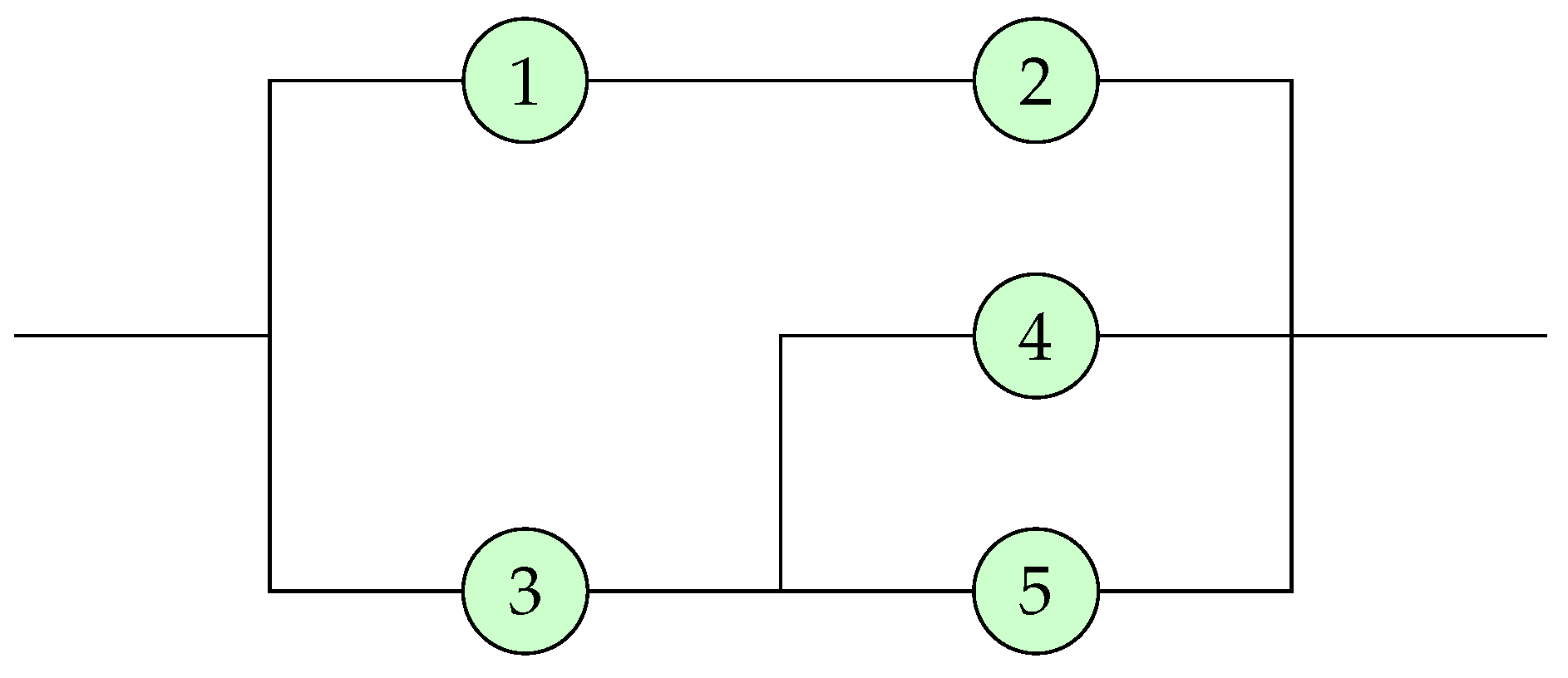
Figure 2.
Exact value of for Part (b) of Example 2 for various values of
Disclaimer/Publisher’s Note: The statements, opinions and data contained in all publications are solely those of the individual author(s) and contributor(s) and not of MDPI and/or the editor(s). MDPI and/or the editor(s) disclaim responsibility for any injury to people or property resulting from any ideas, methods, instructions or products referred to in the content. |
© 2023 by the authors. Licensee MDPI, Basel, Switzerland. This article is an open access article distributed under the terms and conditions of the Creative Commons Attribution (CC BY) license (http://creativecommons.org/licenses/by/4.0/).
Copyright: This open access article is published under a Creative Commons CC BY 4.0 license, which permit the free download, distribution, and reuse, provided that the author and preprint are cited in any reuse.


