Submitted:
29 May 2023
Posted:
30 May 2023
You are already at the latest version
Abstract
Evaluating the performance of water indices and mapping the spatial distribution of water-related ecosystems are important for monitoring surface water resources. This is particularly the case for Ethiopia since there is limited information available on water resources development over time despite its relevance for the people and ecosystems. To address this problem, this paper evaluates the performance of seven water indices for country-scale surface water detection based on high spatial and multi-temporal resolution Sentinel-2 data, processed using the Google Earth Engine cloud computing system. Results show that the water index (WI) and automatic water extraction index with shadow (AWEIsh) are the most accurate ones to extract surface water. Comparisons are based on qualitative visual inspections and quantitative accuracy indicators. For the latter, WI and AWEIsh obtained kappa coefficients of 0.96 and 0.95, respectively, and an overall accuracy of 0.98 each. Both indices accounted for similar spatial coverages of surface waters with 82,650 km2 (WI) and 86,530 km2 (AWEIsh) for the whole of Ethiopia.
Keywords:
Sentinel-2
; remote sensing
; Google Earth Engine
; large-scale
; water resource
1. Introduction
1.1. Water resources and the Sustainable Development Goals
Land surface water is one of the most decisive natural resources substantially changing in spatiotemporal terms, particularly because of land use and land cover dynamics as well as climate change. Land surface water encompasses streams, rivers, ponds, reservoirs, lakes, wetlands and other inland water bodies [1,2]. In spite of its limited extent, particularly in semi-arid and arid regions of the globe, land surface water is a resource for numerous human uses (e.g., drinking water supply, sanitation and hygiene), ensures irrigation agriculture, or is used for hydropower production and industrial use. In addition, it maintains and supports biodiversity and provides essential and diverse ecosystem services [3,4,5]. Surface water resources also play a vital role in the climate system and the hydrological cycle [6,7]. However, water-related ecosystems are fragile and vulnerable to anthropogenic impacts and climate change [8]. The biodiversity of water-related ecosystems continues to deteriorate at an alarming rate [9]. Associated with climate change are hydrological extremes such as flooding or droughts, and emerging water-related diseases, both leading to increasing losses of lives. Therefore, timely monitoring of regional-scale surface water resources is critical for policy and decision-making processes for its sustainable use and management [10,11].
Global initiatives and policy frameworks like the Sustainable Development Goals (SDGs) and the Aichi Biodiversity Targets under the Convention on Biological Diversity (CBD) aim to ensure sustainable development of water resources, to reduce human impact, and prevent the loss of biodiversity [12,13]. Especially, the SDG 6 “Clean water and sanitation” and its target 6.6 “Protect and restore water-related ecosystems” emphasize the need to quantify its indicator 6.6.1 “Change in the extent of water-related ecosystems over time” [14]. Thus, having the aforementioned potential conflicts in mind, this study contributes to quantifying the spatial distribution of the extent of water-related ecosystems at regional-scale for Ethiopia.
Ethiopia has significant surface water resources with eight river basins, one lake basin and three dry basins (Figure 1). A strong rainfall gradient separates the central and western highlands with abundant annual rainfall of up to 1200 mm from the arid southeast, east and northeast, which receive 200 mm and below [15]. Therefore, surface water resources are comparatively less available in the eastern part of Ethiopia (especially in the Awash basin) while the western part with the Abay (Blue Nile) river basin has large water resources. In contrast to the importance of water resources for human well-being and the country’s ecosystems, monitoring systems for the availability of surface water and hydrological flows are in poor condition and sometimes unreliable or malfunctioning [16]. A country-wide continuous assessment of a water resource indicator as requested as part of SDG6 is not in place.
1.2. Remote sensing for monitoring water resources
In contrast to in situ measurements, satellite remote sensing is an effective and efficient tool for monitoring and mapping surface water distributions. It allows covering a wide range of spatial and temporal scales because of its accessibility, repeatability, geospatial consistency, and global coverage [17,18]. Today’s remote sensing applications are characterized by a multitude of high-resolution sensor techniques, often analyzed by powerful cloud computing systems.
Google Earth Engine is such a cloud computing platform for global-scale analyses. It provides access to a range of satellite imagery, particularly Landsat and Sentinel-2 products and facilitates high-performance computing for social and environmental analysis, including water monitoring [19]. The unique band characteristics and spectral response methods of Sentinel-2 data are specifically helpful to detect surface water bodies from the background [20].
Surface water can be detected using multi-spectral satellite imageries on the base of the significantly lower infrared reflectance of water compared to other land cover types. Hence, based on this wavelength, numerous approaches have been developed for extracting surface water from remote sensing imageries.
The water indices method is a common classification method using multi-bands [17]. It is easy to use and quick to calculate [21]. Further indices include the normalized difference water index (NDWI) of McFeeters [22], the modified normalized difference water index (MNDWI) of Xu [23] and the land surface water index (LSWI) of Xiao et al. [24]. All these indices have been widely used in Landsat 5 Thematic Mapper (TM) and Landsat 7 Enhanced Thematic Mapper (ETM+) imagery analyses. They are easy to compute and rely on only two input bands. Feyisa et al. [25] developed the automatic water extraction with no shadow (AWEInsh) using four bands (green, near infrared (NIR), short wave infrared1 (SWIR1), and SWIR2). The AWEIsh additionally utilizes the blue band. AWEIsh is designed for shadows from mountains, buildings, and clouds. The sentinel water index (SWI) proposed by Jiang et al. [20] is computed using red-edge1 and SWIR1 bands of Sentinel-2.
A comparative performance analysis of these water indices for Ethiopia is missing, particularly for the more recent Sentinel-2 data. Choosing the best index for large-scale surface water detection is difficult due to inconsistent results obtained from various indices and unstable threshold values to differentiate water from non-water, which is changing with location and scene [26]. Hence, the objective of this work is to demonstrate the potential of water index methods and select the best-performing indices for detecting surface water fractions using high-resolution and multi-temporal Sentinel-2 data at the country scale. The indices are calculated using the Google Earth Engine. We investigate the spatial distribution of water resources in Ethiopia and monitor surface water resources in relation to the fulfillment of SDG 6.
2. Materials and Methods
2.1. Description of the study area
Ethiopia has 12 major basins with all river basins experiencing water shortage from time to time, except the Abay basin (Figure 1). In the eastern part of Ethiopia, surface water resources are limited since almost no perennial rivers are found below 1,500 m a.s.l. Ethiopia’s 12 major lakes cover around 7,300 km2. Lake Tana (in the Abay basin) is the largest one, and it is the main water source of the Nile River. Most other lakes are saline and located in the Rift Valley.
2.2. Surface water extraction
The methods of water extraction with water indices are implemented starting with (1) data acquisition of Sentinel-2 optical imagery; followed by (2) data pre-processing including the application of cloud/shadow masking and filtering; (3) feature sample collection for performance evaluation; (4) calculation of water indices, and finally (5) performance evaluation of water indices.
(1) Data acquisition
We use Sentinel-2 data from December 01st, 2021 to November 30th, 2022. It is acquired by the Copernicus program in the Earth Observation program of the European Union, which provides multi-spectral data in the visible, near-infrared, and shortwave infrared parts of the spectrum, a total of 13 bands. The granules cover 100 by 100 km2 with a spatial resolution of 10 m (bands blue (B2), green (B3), Red (B4), and NIR (B8), 20 m (red edge 1 (B5), red edge 2 (B6), red edge 3 (B7), red edge 4 (B8a), SWIR 1 (B11), and SWIR 2 (B12) and 60 m (aerosols (B1), water vapor (B9), and cirrus (B10)) for the most widely available Level-1C standard product. The temporal resolution or the revisit frequency of each individual Sentinel-2 satellite is 10 days and the combined constellation revisit is 5 days.
(2) Data pre-processing
Once Sentinel-2 imagery is acquired, it is pre-processed using the cloud/shadow mask function in Google Earth Engine cloud computing processing [27]. Processing is performed in all spectral bands at 60 m spatial resolution. The cloud mask detected cloud-free and cloudy pixels, including both dense clouds and cirrus clouds. After all filtering steps, each corresponding spectral band is resampled in a radiometric interpolation at spatial resolutions of 10 m and 20 m. Thus, all these pre-processing steps contribute to the identification of cloud-free pixels.
(3) Feature sample collection
Georeferenced samples from Sentinel-2 and coincident high-resolution imagery and OpenStreetMap data in Google Earth Engine are collected for accuracy assessments. These samples are collected throughout the entire study area using a stratified random sampling approach. Features are collected from both water and non-water areas, respectively. Water bodies are additionally stratified by size and type, and features in each sample are separated by a minimum distance of 500 m to reduce spatial autocorrelation. A total of 2,480 feature samples are collected in October 2022.
(4) Calculating water indices
Seven water indices are calculated in the Google Earth Engine computing system using the equations presented in Table 1. All indices have originally been developed for Landsat-based index classification except for SWI.
(5) Performance evaluation
Accuracy assessments are carried out to determine whether or not the results of surface water extraction are acceptable. In this study, qualitative (visual) and quantitative assessments are undertaken. In the visual assessment, the magnitude of continuousness and the smoothness of the boundary of water bodies are assessed and cross-checked with reference data. The quantitative assessment is carried out using the 2,480 feature sample points. Indicators of evaluation include producer accuracy, user accuracy, overall accuracy, and Kappa coefficient.
Confusion matrices, the common method of describing the accuracy of the classification [28], are used to compare the reference data and the corresponding classification outputs on a category-by-category basis. According to Lillesand et al. [28], user accuracy is computed by dividing the number of correctly classified pixels in each category by the total number of pixels that are classified in that category (the row total), which is known as the specificity or true negative rate, and the complement of the commission error. The producer accuracy is obtained by dividing the number of correctly classified pixels in each category (on the major diagonal) by the number of training set pixels used for that category (the column total), which is known as the sensitivity or true positive rate, and the complement of the omission error. The Kappa coefficient of the agreement is used for a multivariate statistical measure that can be used to test classification accuracy. The user accuracy, producer accuracy, overall accuracy, and Kappa coefficient are computed including the confusion matrix for the classification in Google Earth Engine computing. Then, based on the detailed visual inspection and the highest values of the accuracy indicators for the validation datasets, the optimum thresholds are determined that separate water and non-water pixels. Finally, based on the aforementioned indicators of accuracy, the better-performing indices are selected and then used to quantify the spatial distribution of surface water resources in Ethiopia.
3. Results
3.1. Visual assessment of water indices
The results of water detection using seven indices for specific locations and the whole of Ethiopia are presented in Figure 3, Figure 4 and Figure 5. As can be seen, particularly in areas #1 and #3, where the surrounding areas are vegetated areas and urban areas, WI and AWEIsh are relatively better at detecting surface water. SWI is less good as there is some misclassification as water bodies (Figure 3, #1 and #2). NDWI is relatively less effective than MNDWI because of some unclassified water pixels, especially in area #1 and #3. In our case, AWEInsh only detects large water bodies, and LSWI is also unable to detect water bodies correctly. In flat areas, WI and AWEIsh are more effective to detect rivers compared to other water indices (Figure 4). MNDWI is also superior in these flat and less vegetated areas, while NDWI is less able to map the rivers. As can also be seen in Figure 4, SWI detected the river but misclassified non-water bodies as water bodies. AWEInsh and NDWI are unable to identify rivers and small water bodies. Therefore, in this large-scale water detection experiment using Sentinel-2 data in Google Earth Engine, the WI and AWEIsh are the best-performing water indices for surface water detection from a visual assessment point of view.
Performance evaluation of water indices
The accuracy assessments of each water index with accuracy indicators are presented in Table 3. As can be seen in Table 3, the detection of surface water bodies is more difficult than that of non-water bodies. The water producer’s accuracy ranges from 0.30 to 0.98, whereas non-water producer’s accuracy ranges from 0.91 to 0.98. All indices, except LSWI, have a satisfying classification accuracy >0.85 with regard to the overall accuracy, producer’s accuracy, user’s accuracy, and Kappa coefficient. The WI achieves the highest accuracy with a Kappa coefficient and overall accuracy of 0.96 and 0.98, respectively. All other indicators, except for the LSWI, have only slightly worse performance criteria. The difference in accuracy between the LSWI and the other indices is striking. This index is the least-performing one with an overall accuracy and Kappa coefficient of 0.82 and 0.31, respectively. Overall, the AWEIsh and particularly WI outperform the other indices regarding accuracy indicator performances depicted by the heat map in Table 3, whereby it must be said that the differences between six of the seven indices are in part only marginal. Together with the information from the visual assessment, we conclude that in this study, the WI and AWEIsh are the most accurate water indices using the high and multi-temporal resolution of Sentinel-2 data for surface water detection in Ethiopia.
Finally, the surface water coverage is calculated using the seven indices across Ethiopia. As can be seen, WI, AWEIsh, and MNDWI indices extract more or less similar surface water coverages of 82,650, 86,530, and 88,160 km2, respectively. Slightly deviating is the coverage estimated by NDWI (79,650 km2). Completely different are the remaining coverages derived by the AWEInsh (51,800 km²), SWI (111,500 km2) and LSWI (207,520 km2).
4. Discussion
Many water indices have been used in analyzing Landsat imagery (e.g., NDWI [22], LSWI [24], MNDWI [23], AWEI [25], and WI [17]). In Ethiopia, for example, Sisay et al. [29] estimated the development of lake sizes over time of three lakes in the South part of the country using Landsat data. An analysis for the entire country is not at hand, to our best knowledge. The launch of the Sentinel constellation by the European Space Agency (ESA) under the Copernicus program is a breakthrough moment as it provides access to free and high-resolution imagery. Therefore, we calculated several Landsat-based water indices on the national level of Ethiopia using Sentinel-2 data.
In the visual assessment, our results show that the WI and AWEIsh indices have a superior accuracy in surface water detection. They are more effective to detect surface water in urban and vegetated areas, despite that the detection in such areas is commonly difficult due to shadows [25]. Shadows in urban areas are often misclassified as water bodies, as they have similar low reflectivity characteristics to water bodies [30]. Fischer et al. [17] state that WI and AWEIsh performed best, the MNDW and AWEInsh performed less accurately, and NDWI the least. In our study MNDWI is more effective than NDWI, AWEInsh and SWI in detecting rivers and small water bodies. The MNDWI is an improved version of the NDWI in that it uses the SWIR band instead of the NIR band that is used in the NDWI to normalize the water and vegetation indices [23]. NDWI is less sensitive to small water bodies and rivers and is also affected by noise from urban and vegetated areas. As a result, it is unable to detect part of the Awash River and small water bodies in the Bahir Dar area (Figure 3 and Figure 4). The contrast between water and land is acceptable for MNDWI, although it is less accurate than WI and AWEI in predicting the fractional cover of small water bodies or small streams [30]. SWI is better than NDWI, AWEInsh, and LSWI for detecting small water bodies and river channels. However, it is challenged by the elimination of shadow noise from surrounding non-water features. Jiang et al. [20] also observed that SWI is better than NDWI at detecting wide river channels.
The accuracy of the water indices are evaluated quantitatively in terms of different accuracy indicators: producer’s accuracy, user’s accuracy, overall accuracy, and kappa coefficient. Surface water is more difficult to detect than non-water surfaces. This is because water is transparent and changes color depending on the depth, color and amount of sediment it contains. Our result shows that WI and AWEIsh are the most accurate water indices. A similar result was observed in four cases studies in Switzerland, Ethiopia, South Africa, and New Zealand, where AWEIsh achieved water user and producer accuracies of 0.96-0.99 and 0.91-0.99%, respectively [25]. Similarly, AWEIsh achieved a kappa coefficient of 0.97 in Ethiopia, and AWEInsh was also detected in a shadow-free image from Denmark with water user’s and producer’s accuracy of 0.98 and 0.92, respectively [25]. Fisher et al. [17] reported – close to our results – overall accuracies of 0.98, 0.97, and 0.95 for WI, MNDWI, and NDWI for images from eastern Australia. Liu et al. [30] also observed that WI achieved an overall accuracy of 0.96 and a kappa coefficient of 0.89, and AWEIsh also performed well with an overall accuracy of 0.96 and a kappa coefficient of 0.89. In this study, LSWI performs worse due to the limitation of the index in interpreting Sentinel-2 data. It is also heavily influenced by the background noise of non-water features in the study area.
Overall, the performance evaluation criteria in our study are common and acceptable for evaluating the results of surface water detection using water indices [17,25]. The results present are even slightly higher than those of previous works, which range from 0.94 to 0.98 in overall accuracy, except for LSWI. This is perhaps due to the use of relatively higher spatial and spectral resolution of the Sentinel-2 data with Google Earth Engine processing. In addition, Sentinel-2’s unique band characteristics and spectral response methods are likely more effective than Landsat imagery at detecting water bodies from the background [20].
The best-performing indices, WI and AWEIsh, are efficient and replicable in Sentinel-2 data using Google Earth Engine computing. Even though they are specifically designed for Landsat sensors [17,25], they are also effective in producing high-quality maps for large-scale surface water detection using high-resolution Sentinel-2 imagery. Consequently, these methods are useful for policymakers and stakeholders in water resources monitoring, also in the light of missing monitoring efforts of SDG6 for Ethiopia.
5. Conclusion
This paper demonstrates that the qualitative and quantitative accuracy of WI and AWEIsh are sufficient for operational surface water detection on a national scale in Ethiopa. High-resolution and multi-temporal Sentinel-2 data have an important potential application in large-scale surface water detection. Our results confirm that water indices using Sentinel-2 data produce reliable surface water coverage assessments and that the application of water indices could successfully contribute to the achievement of SDG 6 at the regional level, as they are useful for guiding conservation efforts and the sustainable use and management of surface water resources.
However, any approach of surface water detection that only considers remote sensed imagery has difficulties in making future projections of surface water coverage, as images are always from the past. For future projections, for example if information is needed on climate or land use change effects on surface water resources, dynamic variables that change over time should complement surface water detection. This likely includes hydro-meteorological variables from weather forecasts or climatic projections as well as dynamic land use features of land use projections. Such information should be merged with satellite imagery to allow for future projections. For this task, we see a particular benefit for method and data fusion techniques using machine learning methods, which have been provided promising results in the recent past for surface water detection [31,32].
Author Contributions
Conceptualization, MT and LB; methodology, MT; formal analysis, MT; validation, MT and LB; supervision, LB; draft preparation, MT; review and editing, LB. Both authors have read and agreed to the published version of the manuscript.
Funding
This research was funded by German Academic Exchange Service (DAAD), funding program/-ID: Research Grants - Doctoral Programmes in Germany, 2022/23 (57588370).
Data Availability Statement
The data and code presented in this study are available on request from the corresponding author.
Acknowledgments
MT would like to thank the German Academic Exchange Service (DAAD) for its financial support.
Conflict of interest: The authors declare no competing interests.
References
- Pekel, J. F.; Cottam, A.; Gorelick, N.; Belward, A. S. High-Resolution Mapping of Global Surface Water and Its Long-Term Changes. Nature, 2016, 540, 418–422. [CrossRef]
- Vandas, S.; Winter, T.C.; Battaglin, W,A. Water and the Environment. American Geosciences Institute Environmental Awareness, 2002, 20-23.
- Dudgeon, D.; Arthington, A. H.; Gessner, M. O.; Kawabata, Z. I.; Knowler, D. J.; Lévêque, C.; Naiman, R. J.; Prieur-Richard, A. H.; Soto, D.; Stiassny, M. L. J.; et al. Freshwater Biodiversity: Importance, Threats, Status and Conservation Challenges. Biological Reviews of the Cambridge Philosophical Society, 2006, 163–182. [CrossRef]
- Zedler, J. B.; Kercher, S. Wetland Resources: Status, Trends, Ecosystem Services, and Restorability. Annual Review of Environment and Resources, 2005, 39–74. [CrossRef]
- Brauman, K. A. Hydrologic Ecosystem Services: Linking Ecohydrologic Processes to Human Well-Being in Water Research and Watershed Management. Wiley Interdisciplinary Reviews: Water, 2015, 2, 345–358. [CrossRef]
- Chahine, M. T. The Hydrological Cycle and Its Influence on Climate. Nature, 1992, 359, 373-380.
- Tranvik, L. J.; Downing, J. A.; Cotner, J. B.; Loiselle, S. A.; Striegl, R. G.; Ballatore, T. J.; Dillon, P.; Finlay, K.; Fortino, K.; Knoll, L. B.; et al. Lakes and Reservoirs as Regulators of Carbon Cycling and Climate. Limnology and Oceanography, 2009, 54, 2298–2314. [CrossRef]
- Vörösmarty, C. J.; Green, P.; Salisbury, J.; Lammers, R. B. Global Water Resources: Vulnerability from Climate Change and Population Growth. Science, 2000, 289, 284-288. [CrossRef]
- Collen, B.; Whitton, F.; Dyer, E. E.; Baillie, J. E. M.; Cumberlidge, N.; Darwall, W. R. T.; Pollock, C.; Richman, N. I.; Soulsby, A. M.; Böhm, M. Global Patterns of Freshwater Species Diversity, Threat and Endemism. Global Ecology and Biogeography, 2014, 23, 40–51. [CrossRef]
- Morss, R. E.; Wilhelmi, O. v.; Downton, M. W.; Gruntfest, E. Flood Risk, Uncertainty, and Scientific Information for Decision Making: Lessons from an Interdisciplinary Project. Bulletin of the American Meteorological Society, 2005, 86, 1593–1601. [CrossRef]
- Giardino, C.; Bresciani, M.; Villa, P.; Martinelli, A. Application of Remote Sensing in Water Resource Management: The Case Study of Lake Trasimeno, Italy. Water Resources Management, 2010, 24, 3885–3899. [CrossRef]
- Griggs, D. Sustainable Development Goals for People and Planet. Nature, 2013, 495, 1-3.
- CBD. Convention on Biological Diversity for Aichi Biodiversity Targets, 2010. http://www.cbd.int/sp/targets/.
- Dickens, C.; Rebelo, L. M.; Nhamo, L. Guidelines and indicators for Target 6.6 of the SDGs: Change in the extent of water-related ecosystems over time. Report by the International Water Management Institute. CGIAR Research Program on Water, Land, and Ecosystems (WLE), 2017, 4-10.
- Berhanu, B.; Seleshi, Y.; Melesse, A. M. Surface Water and Groundwater Resources of Ethiopia: Potentials and Challenges of Water Resources Development. Nile River Basin: Ecohydrological Challenges, Climate Change and Hydropolitics, Springer International Publishing, 2014, 97–117. [CrossRef]
- Dile, Y. T.; Tekleab, S.; Kaba, E. A.; Gebrehiwot, S. G.; Worqlul, A. W.; Bayabil, H. K.; Yimam, Y. T.; Tilahun, S. A.; Daggupati, P.; Karlberg, L.; et al. Advances in Water Resources Research in the Upper Blue Nile Basin and the Way Forward: A Review. Journal of Hydrology, 2018, 407–423. [CrossRef]
- Fisher, A.; Flood, N.; Danaher, T. Comparing Landsat Water Index Methods for Automated Water Classification in Eastern Australia. Remote Sensing of Environment, 2016, 175, 167–182. [CrossRef]
- Mueller, N.; Lewis, A.; Roberts, D.; Ring, S.; Melrose, R.; Sixsmith, J.; Lymburner, L.; McIntyre, A.; Tan, P.; Curnow, S.; et al. Water Observations from Space: Mapping Surface Water from 25 Years of Landsat Imagery across Australia. Remote Sensing of Environment, 2016, 174, 341–352. [CrossRef]
- Gorelick, N.; Hancher, M.; Dixon, M.; Ilyushchenko, S.; Thau, D.; Moore, R. Google Earth Engine: Planetary-Scale Geospatial Analysis for Everyone. Remote Sensing of Environment, 2017, 202, 18–27. [CrossRef]
- Jiang, W.; Ni, Y.; Pang, Z.; Li, X.; Ju, H.; He, G.; Lv, J.; Yang, K.; Fu, J.; Qin, X. An Effective Water Body Extraction Method with New Water Index for Sentinel-2 Imagery. Water, 2021, 13. [CrossRef]
- Ryu, J. H.; Won, J. S.; Duck Min, K. Waterline Extraction from Landsat TM Data in a Tidal Flat A Case Study in Gomso Bay, Korea. Remote Sensing of Environment, 2002, 83, 442–456.
- McFeeters, S. K. The Use of the Normalized Difference Water Index (NDWI) in the Delineation of Open Water Features. International Journal of Remote Sensing, 1996, 17 (7), 1425–1432. [CrossRef]
- Xu, H. Modification of Normalised Difference Water Index (NDWI) to Enhance Open Water Features in Remotely Sensed Imagery. International Journal of Remote Sensing, 1996, 17, 1425–1432. [CrossRef]
- Xiao, X.; Boles, S.; Liu, J.; Zhuang, D.; Liu, M. Waterline Extraction from Landsat TM Data in a Tidal Flat A Case Study in Gomso Bay, Korea. Remote Sensing of Environment, 2002, 83 442–456.
- Feyisa, G. L.; Meilby, H.; Fensholt, R.; Proud, S. R. Automated Water Extraction Index: A New Technique for Surface Water Mapping Using Landsat Imagery. Remote Sensing of Environment, 2014, 140, 23–35. [CrossRef]
- Ji, L.; Zhang, L.; Wylie, B. Analysis of Dynamic Thresholds for the Normalized Difference Water Index. Photogrammetric Engineering and Remote Sensing, 2009, 75, 1307–1317. [CrossRef]
- Sentinel. Sentinel-2 MSI User Guide. https://sentinels.copernicus.eu/web/sentinel/user-guides/sentinel-2-msi, Accessed 4 December 2022.
- Lillesand, T. M.; Kiefer, R. R. W.; Chipman, J. W. Remote Sensing and Image Interpretation. 6th ed. New York: Wiley, 2008.29. Sisay, A. Remote Sensing Based Water Surface Extraction and Change Detection in the Central Rift Valley Region of Ethiopia. In Int. J. of Sustainable Water and Environmental Systems, 2017, 9,1, 01-07.
- Liu, H.; Hu, H.; Liu, X.; Jiang, H.; Liu, W.; Yin, X. A Comparison of Different Water Indices and Band Downscaling Methods for Water Bodies Mapping from Sentinel-2 Imagery at 10-M Resolution. Water, 2022, 14, 1-15. [CrossRef]
- Yang, L.; Driscol, J.; Sarigai, S.; Wu, Q.; Lippitt, CD.; Morgan, M. Towards Synoptic Water Monitoring Systems: A Review of AI Methods for Automating Water Body Detection and Water Quality Monitoring Using Remote Sensing. Sensors, 2022, 22, 6, 1-48. https://www.mdpi.com/1424-8220/22/6/2416.
- Li, J.; Ma, R.; Cao, Z.; Xue, K.; Xiong, J.; Hu, M.; Feng, X.. Satellite detection of surface water extent: A review of methodology. Water, 2022, 14, 7, 1-18. https://www.mdpi.com/2073-4441/14/7/1148.
Figure 1.
Main water bodies with basins of Ethiopia (own figure, source: Ethiopia Geospatial Institute).
Figure 1.
Main water bodies with basins of Ethiopia (own figure, source: Ethiopia Geospatial Institute).
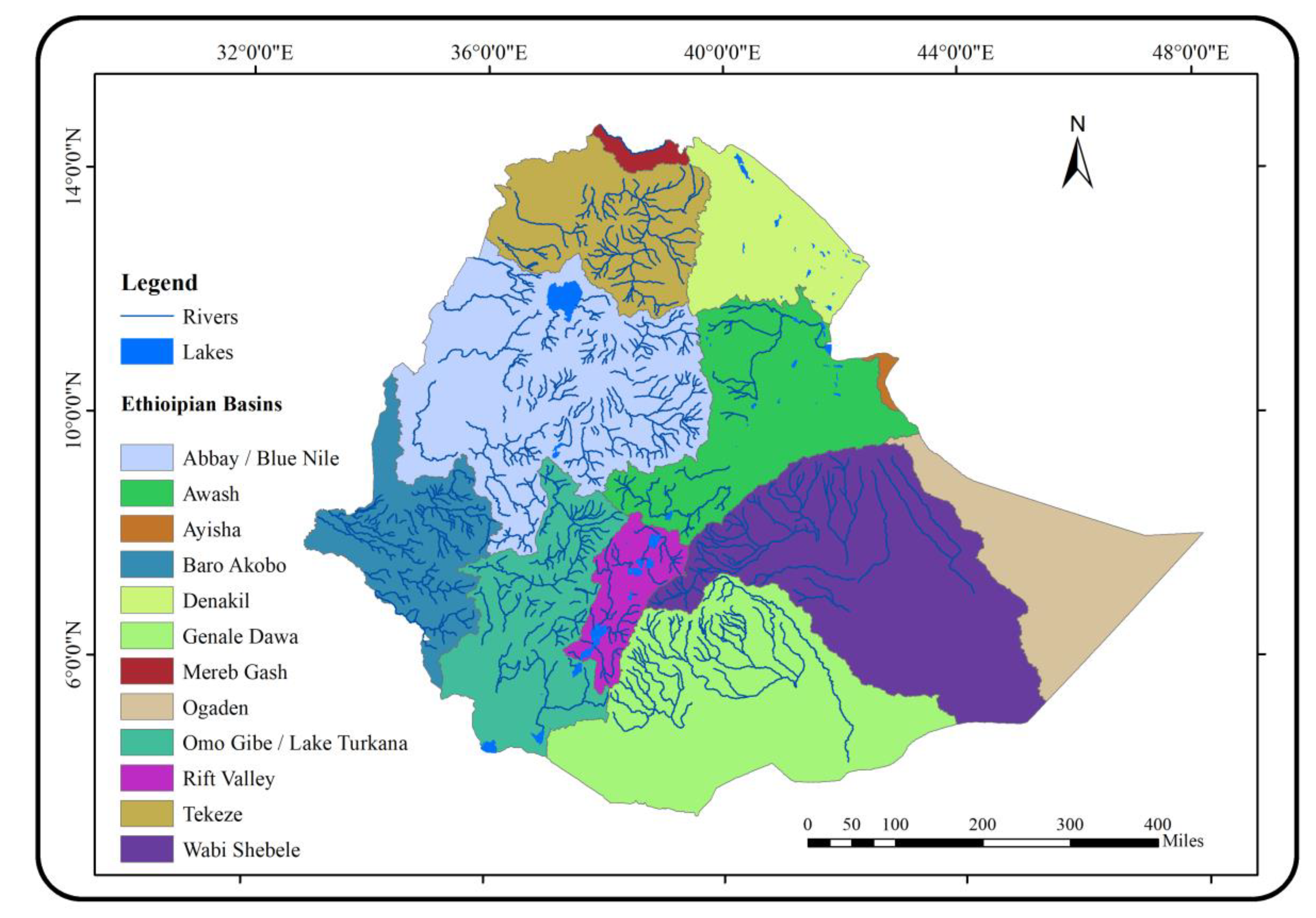
Figure 3.
Specific map section for visual assessment and comparison of water indices outputs for part of the Bahir Dar area.
Figure 3.
Specific map section for visual assessment and comparison of water indices outputs for part of the Bahir Dar area.
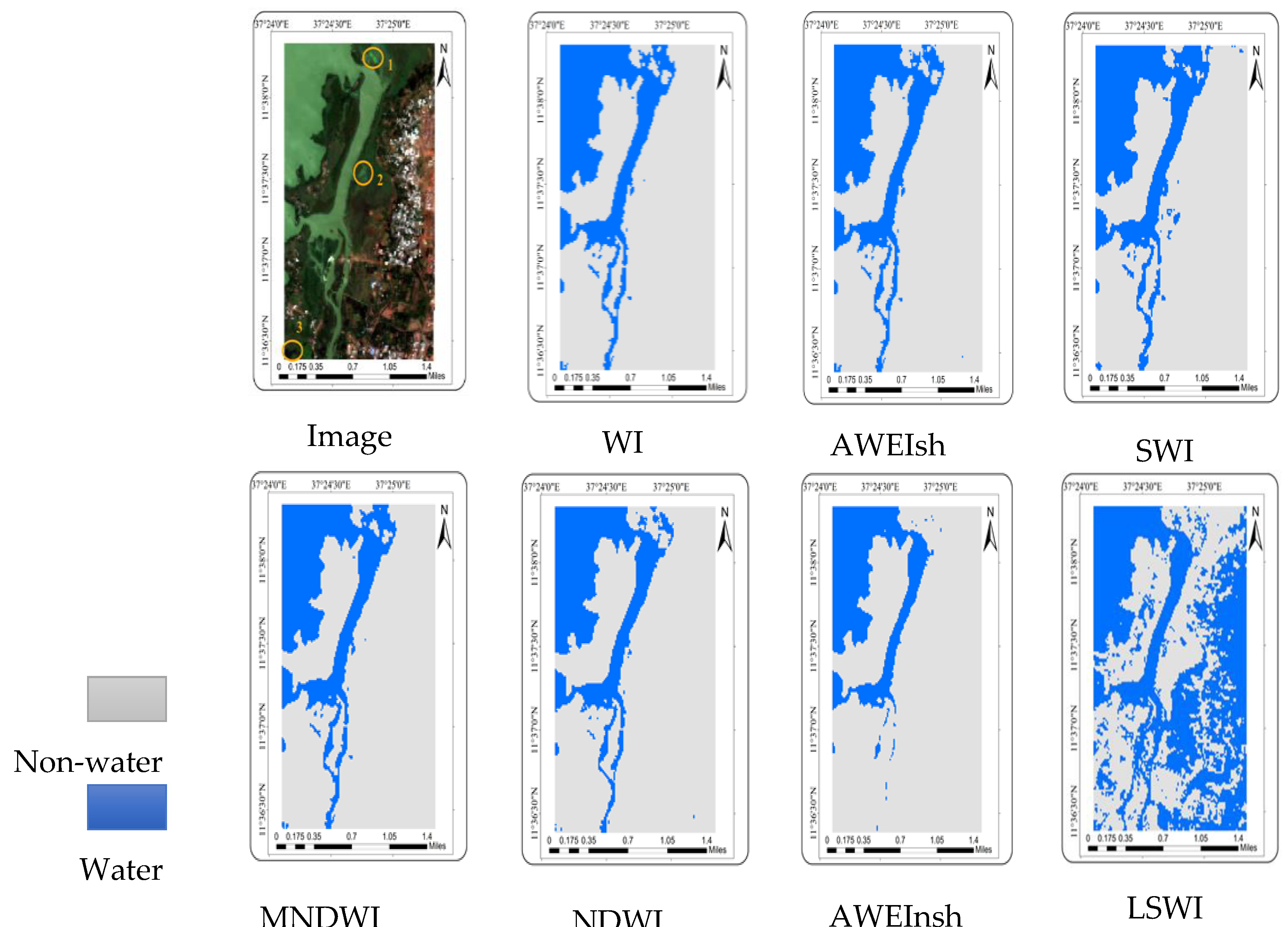
Figure 4.
Specific map section for visual assessment and comparison of water indices outputs for the Awash river reach.
Figure 4.
Specific map section for visual assessment and comparison of water indices outputs for the Awash river reach.
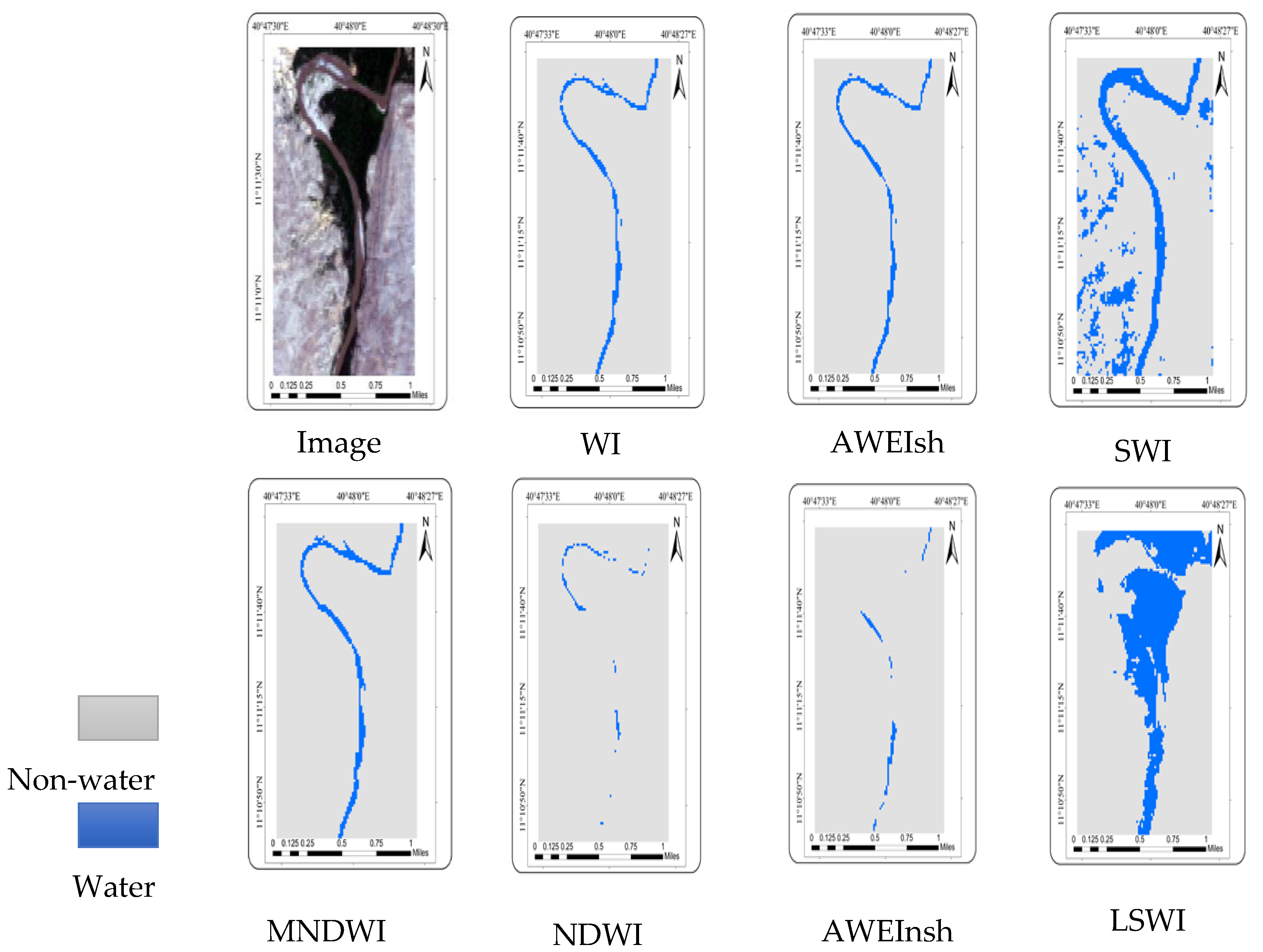
Figure 5.
Country-scale map of surface water coverage using best-performing water indices.
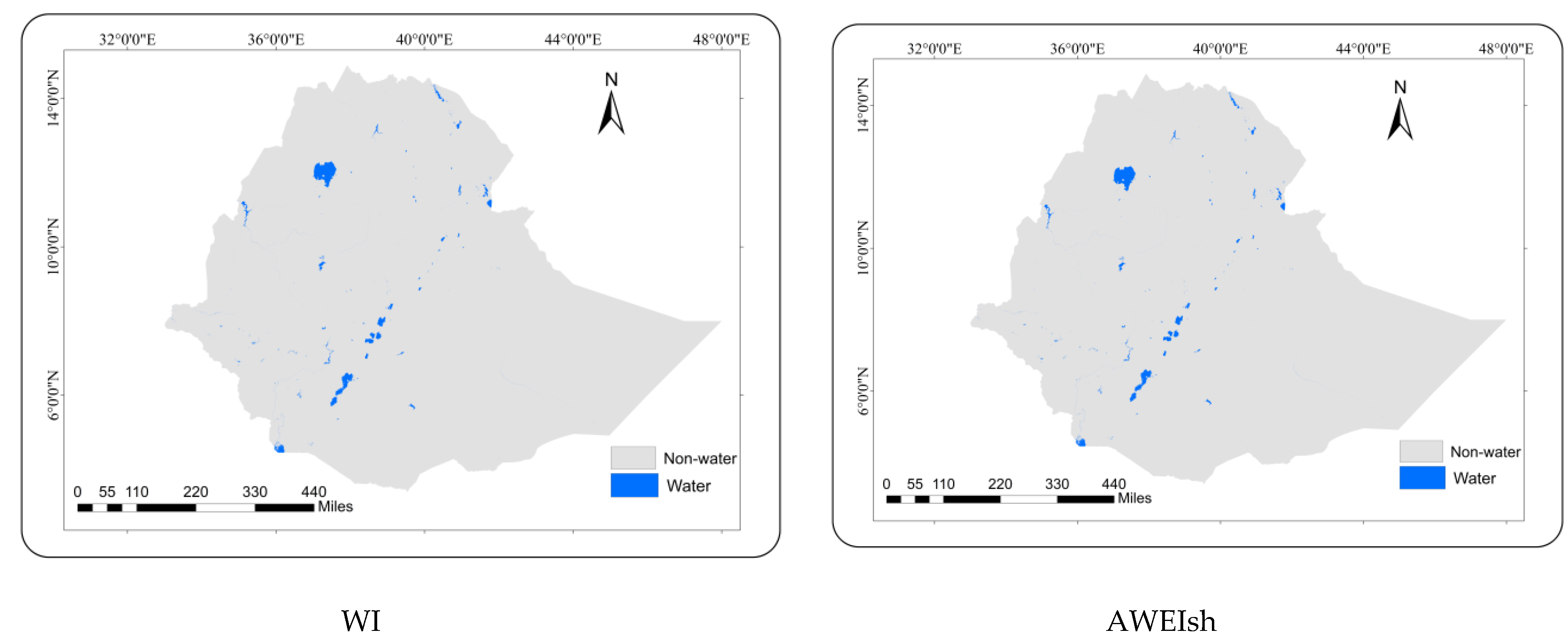

Table 1.
Water index methods.
| Index | Index name | Source | Equation |
| NDWI | Normalized Difference Water Index | McFeeters (1996) | |
| MNDWI | Modified Normalized Difference Water Index | Xu (2006) | |
| AWEInsh | Automated Water Extraction Index non shadow | Feyisa et al. (2014) | (4*(Green-SWIR1))-(0.25*NIR+(2.75*SWIR2)) |
| AWEIsh | Automated Water Extraction Index shadow | Feyisa et al. (2014) | (Blue+2.5*Green-1.5*(NIR+SWIR1)-0.25*SWIR2) |
| WI | Water Index | Fischer et al. (2015) | (1.7204+171*Green+3*Red-70*NIR-45*SWIR1-71*SWIR2) |
| SWI | Sentinel Water Index | Jiang et al. (2021) | |
| LSWI | Land Surface Water Index | Xiao et al. (2002) |
Table 3.
Heat map of classification accuracies and Kappa coefficients of water indices (acc=accuracy).
Table 3.
Heat map of classification accuracies and Kappa coefficients of water indices (acc=accuracy).
| Producer acc | Producer acc | User acc | User acc | Overall acc | Kappa coeff | |
| Water | Non-water | Water | Non-water | |||
| NDWI | 0.87 | 0.95 | 0.94 | 0.95 | 0.94 | 0.89 |
| MNDWI | 0.94 | 0.96 | 0.95 | 0.96 | 0.96 | 0.93 |
| AWEInsh | 0.97 | 0.97 | 0.96 | 0.97 | 0.97 | 0.94 |
| AWEIsh | 0.98 | 0.97 | 0.96 | 0.98 | 0.98 | 0.95 |
| WI | 0.97 | 0.98 | 0.97 | 0.98 | 0.98 | 0.96 |
| SWI | 0.93 | 0.97 | 0.95 | 0.97 | 0.97 | 0.94 |
| LSWI | 0.3 | 0.91 | 0.37 | 0.88 | 0.82 | 0.31 |
Disclaimer/Publisher’s Note: The statements, opinions and data contained in all publications are solely those of the individual author(s) and contributor(s) and not of MDPI and/or the editor(s). MDPI and/or the editor(s) disclaim responsibility for any injury to people or property resulting from any ideas, methods, instructions or products referred to in the content. |
© 2023 by the authors. Licensee MDPI, Basel, Switzerland. This article is an open access article distributed under the terms and conditions of the Creative Commons Attribution (CC BY) license (http://creativecommons.org/licenses/by/4.0/).
Copyright: This open access article is published under a Creative Commons CC BY 4.0 license, which permit the free download, distribution, and reuse, provided that the author and preprint are cited in any reuse.


