Hierarchical Network-Based Tracklets Data Association for Multiple Extended Targets Tracking With Intermittent Measurements

The main problem in pursuing multiple extended targets tracking is distinguishing the origins of the measurements. The association of measurements to the possible origins within the target’s extent is difficult, especially for the occlusions or the detection blind zone which cause the intermittent measurements. To solve the problem, a hierarchical network-based tracklets data association algorithm is proposed. At the low level, the min cost network flow model is used to extract possible tracklets from the divided measurement set. At the high-level, the trajectories are estimated from the tracks produced by the previous low level network. The experimental results show that the hierarchical network-based tracklets data association algorithm outperforms the JPDA and RFS-based method when the measurement is intermittently unavailable.

Keywords:

Subject: Computer Science and Mathematics - Information Systems

1. Introduction

Conventional MTT algorithms assume that objects can be represented as points and allow only a single measurement per sensor scan. However, modern high-resolution sensors have revealed the existence of targets that can generate multiple measurements per scan. This challenges the suitability of the conventional point-target assumption. In such scenarios, multi-extended targets tracking (METT) provides a more appropriate approach as it specifically addresses the tracking of targets that can produce multiple measurements per scan. The MTT with more measurement per target is called multiple extended targets tracking (METT)[2].

Data association plays a vital role in multi-target tracking by differentiating between false alarms and actual targets. Incorrect data association can significantly impact the performance of tracking multiple targets. For point targets, several methods for data association have been proposed, which can be found in the referenced source [3]. On the other hand, data association for extended targets involves the challenging task of matching measurements to specific targets, and this complexity increases with the number of targets and measurements. To address this, multiple data association techniques have been developed specifically for multi-extended target tracking (METT) scenarios. It is clear that data association is critical in multi-target tracking, and its approach and complexity differ between point targets and extended targets. Specialized data association techniques are necessary for METT applications.

Vivone introduced a method that incorporates a detector and Joint Probability Data Association (JPDA) tracker specifically designed for METT [4].Additionally, the multi-detection JPDA (MD-JPDA) algorithm was developed to address many-to-one associations in high-resolution radar sensors [5]. However, MD-JPDA suffers from high complexity due to exhaustive combinations of measurements. To mitigate this issue, MD-JIPDA, an extension of MD-JPDA, integrates the existence probability, reducing complexity [6][7].Another approach by Yang focuses on calculating marginal association probabilities for METT without relying on exhaustive hypotheses and partitions [8]. Furthermore, several algorithms based on the random finite sets (RFS) framework have been proposed. These include the Probability Hypothesis Density (PHD) filter [9][10], Cardinalized PHD (CPHD) filter [11], Generalized Labeled Multi-Bernoulli (GLMB) filters[12], and Poisson Multi-Bernoulli Mixture (PMBM)[13]. These RFS-based methods offer both optimal and suboptimal state estimates for multiple extended targets. However, it is important to note that tuning parameters for RFS-based methods may impact system reliability.

In addition, the graphical model formulation is applied to deal with the problem of the METT. Su presents the belief propagation (BP) algorithm to obtain estimators based on a simplified measurement set [14]. In order to get rid of the deviation of the extended state estimation, a METT algorithm based on Loopy Belief Propagation (LBP) is presented in [15].Previously developed METT algorithms rely on continuous measurement availability.

Intermittent measurements are a common occurrence in practical applications due to occlusions, detection blind zones (DBZ), and low frame rates caused by radar operation. To handle subsequent miss-detections, Mahdi proposes the IMM-PHD tracker based on the Probability Hypothesis Density (PHD) algorithm [16], However, this tracker does not output track labels. Another method, the multiple-model multiple hypothesis PHD (MM-MH-PHD) filter, adopts a multiple-model approach to estimate motion states in blind zones [17].In the case of tracking maneuvering targets in blind areas while considering DBZ masking, the MM-GLMB filter is utilized in [18],incorporating a minimum detection speed. However, the above work is not suitable for METT.

In this paper, we propose a hierarchical network framework of the METT with intermittent measurements. The core of our algorithm lies on the association between the reliable tracklets. We exploit a layered network which with respect to the low-level min-cost flow constructed by the clustered measurements set and the high-level min-cost flow constructed by these tracklets. By running the A* algorithm on the low network, we can obtain the reliable tracklets. Then, the minimum cost flow algorithm is employed to get the long trajectories from the directed acyclic graph. Experimental results of intermittent measurements show that the hierarchical network-based tracklets algorithm(ET-HT) is effective. The structure of this paper is as follows.

Section II provides the problem statement, highlighting the need for effective tracking methods. In Section III, detailed information about the ET-HT algorithm is presented, specifically emphasizing the ET-HT data association algorithm. The paper further discusses simulation results in Section IV, demonstrating the effectiveness of the ET-HT algorithm in tracking multiple targets. Finally, Section V serves as the conclusion, summarizing the key findings and contributions of the document.

2. Problem Formulations

The METT problem aims to estimate states and parameters while dealing with measurements from multiple extended targets and the presence of clutter. At each time step k, the states of the multiple extended targets are denoted as

S_{k} = {s_{1, k}, s_{2, k}, . ., s_{N_{T}, k}}

N_{T}

representing the number of extended targets. Each extended target state is defined as

s_{i, k} = {[x_{i, k}, X_{i, k}]}^{T}

. The subset of the state

x_{i, k}

includes the centroid’s location

m_{i, k}

and velocity

{\dot{m}}_{i, k}

of the centroid of the target,

x_{i, k} = {[m_{i, k}, {\dot{m}}_{i, k}]}^{T}

X_{i, k} \in R^{d}

is the extension state that describes the size and shape of the i-th target, in this paper, the dimension of the target extension is set to

d = 2

. At the time step k, the unordered set of measurements containing the clutter and target

Z_{k}

is received by the sensor.

Z_{k} = {z_{1, k}, z_{2, k}, . . ., z_{M_{k}, k}}

, where

M_{k} = \sum_{i}^{N_{T}} M_{i, k} + M_{C, k}

represents the number of measurements.

M_{i, k}

is defined as the total number of measurements that originates from the i-th extended target. The number of clutter

M_{C, k}

is Poisson-distributed with mean

λ_{C}

In multiple extended target tracking, the measurements may intermittently be unavailable at any time. This is due to the occlusions, the detection blind zone or even the low frame rate causes by the work mode of the radar. To cater for the missing measurement, a binary variable representing the existence of the extended target is introduced, inspired by [19].

r_{k} = {r_{1, k}, r_{2, k}, . . ., r_{N_{T}, k}}

, with

r_{i, k} \in {0, 1}

, where the values of 0 and 1 correspond to the loss of the data and the measurement set of the i-th extended target has been successfully received, respectively. The time-homogeneous binary Markov process has a transition probability matrix given by

π^{+} = ({r_{i, k + 1} = n |r_{i, k} = m})_{m, n \in S} = [\begin{matrix} 1 - q_{s, i} & q_{s, i} \\ p_{f, i} & 1 - p_{f, i} \end{matrix}]

(1)

where

S = {0, 1}

is defined as the state space of the Markov process. The parameter

p_{f, i}

and

q_{s, i}

denote the failure rate and recovery rate,

0 < p_{f, i}, q_{s, i} < 1

, so that the Markov process

{r_{k}}_{k \geq 0}

is ergodic. Obviously, a smaller value of

p_{f}

and a larger value of

q_{s}

indicate a more reliable measurement received. Thus, the obtained measurement set of the i-th extended target at the time step k, can be describe as

Z_{i, k} = r_{i, k} {\{z_{i, k}\}}^{M_{i, k}}

(2)

The objective of METT is to calculate the maximum probability data association with intermittent measurements, and recursively estimate the multi-target state given a set of observation.

3. Hierarchical Network-Based Data Association for Multiple Extended Target Tracking

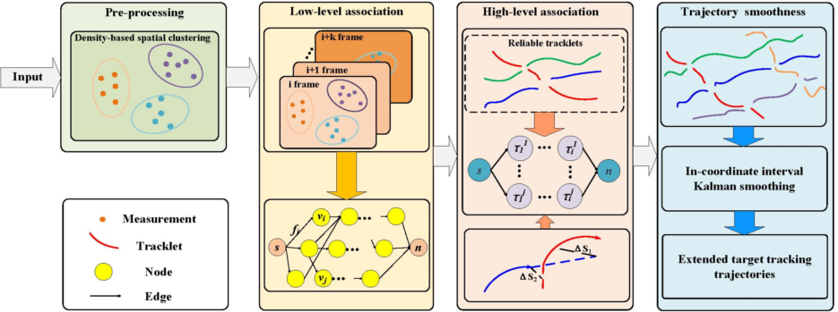
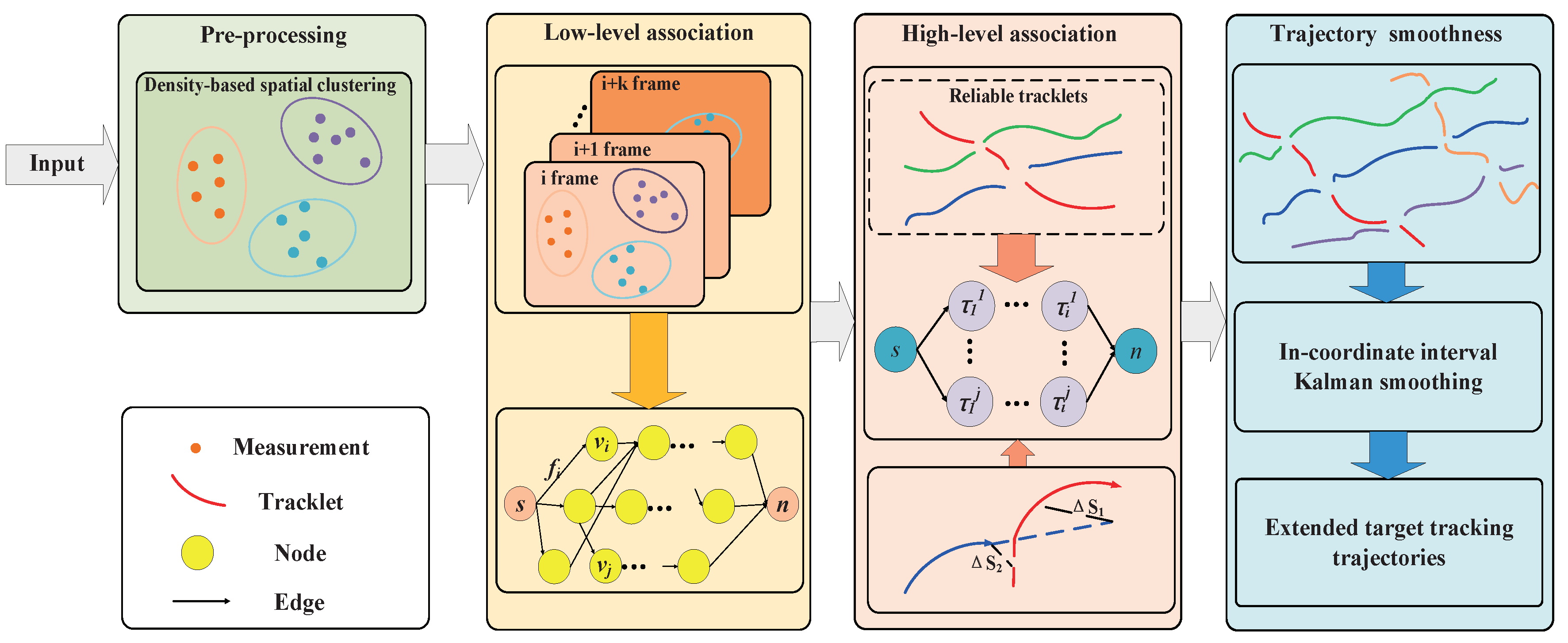
In this paper, we focus on the modeling of multiple extended targets (MET) data association, utilizing a hierarchical dense neighborhood search approach. To achieve this, the Density-based spatial clustering algorithm is employed to divide measurements at a specific time into clusters. Subsequently, a low-level association network is constructed based on the clustering results, enabling the calculation of tracklets. The association of clusters is formulated as a maximum a posteriori (MAP) problem, taking into account target initiation, termination, and false trajectories arising from clutter. At a higher level, the association network estimates trajectories by utilizing the tracklets derived from the low-level network. The paper presents the flowchart of the ET-HT algorithm in Figure 1, illustrating the stepwise process.

3.1. Pre-Processing

Since the set of measurements includes extended targets and clutter, it is necessary to extract the measured data of every extended object in one time step. Consider the properties of the measurements of the extended target that detections are spatially distributed around; the Density-based spatial clustering algorithm is used to partition the set of measurements into multiple partitions. For the set of measurement

Z_{k}

which is received by the sensor at the time k, the set of subpartitions is

Π_{k} = (π_{1, k}, π_{2, k}, \dots π_{N_{π}, k})

(3)

where

N_{π}

is the number of all subpartitions,

π_{i, k}

represents a single subpartition. Note that the traditional partition algorithms include distance partition, subpartition, and K-means clustering. These methods require the specification of the amount of clusters. The density-based spatial clustering can determine the amount of clusters automatically in this paper, based on the intrinsic structure of the set of measurements. The details of the implementation can be found in [20].

3.2. Hierarchical Association

The hierarchical association model consists of low and high-level association network, respectively.

a. low-level association network

Due to the intermittent observations in the extended target tracking system, the extended target trajectories may be divided into several unconnected tracklets. Let

T_{i} = (τ_{i}^{1}, τ_{i}^{2}, \dots, τ_{i}^{n})

represents the i-th extended target trajectory,

τ_{i}^{j}

is defined as the j-th tracklet of the i-th target, and the number of trajectories is unknown.

T = (T_{1}, T_{2}, \dots, T_{m})

is the set of the tracklets. In this section, we denote the set of subpartitions

Π_{1 : k} = (Π_{1}, Π_{2}, \dots, Π_{k})

. The low-level association define

Π_{1 : k}

as the input, and uses the network flow method to generate the tracklets. The key here is to calculate a MAP estimate for

T

with a cluster of measurements set

Π_{1 : k}

T^{*} = arg max \prod_{T} P (T | Π_{1 : k})

(4)

We define

G (V, E)

as a directed acyclic graph, with s denoting the nodes of the graph and n being the set of edges of the graph. This gives the set of graph nodes

V

and

E

, with

v_{i}

defined as a subpartition and each edge

e_{j}

G (V, E)

representing the motion between the subpartitions. In solving the data association process, we use the concept of network flow to represent

f_{i j}

as a directed flow variable from node

v_{i}

to node

v_{j}

, where

f_{s i}

and

f_{j n}

denote the starting flow variable and the ending flow variable, respectively. Each flow in the graph is subject to the following constraints, firstly, the sum of the flows arriving at node v is equal to the sum of the flows leaving this node at the same moment. For any tracklet

τ_{i}^{j}

f_{s i} + \sum_{j : j i \in E} f_{j i} = \sum_{j : i j \in E} f_{i j} + f_{j n}

(5)

Secondly, the cost flow network must ensure that nothing other than a single extended object can be represented at one time. The upper bound of the sum of outgoing flows from node

v_{i}

is set to 1. For any node:

\forall v_{i}, v_{j} \sum f_{i j} < 1

(6)

Considering that targets can appear or disappear anywhere in the cost-flow network, a source node and a sink node are introduced in [21], which are respectively connected to the respective nodes. The source and sink nodes are also subject to a constraint that enforces all the flows starting in s to end in n.

\sum_{i} f_{s i} = \sum_{i} f_{i n}

(7)

Through the network optimization process, Eq.(4) is transformed into an IP problem, and the logarithm of the objective function is given by

\begin{matrix} T^{*} & = arg max \prod_{T} P (T | Π_{1 : k}) \\ = arg max \sum_{T} c_{s i} f_{s i} + c_{i j} f_{i j} + c_{j n} f_{j n} \\ = arg max \sum_{i} c_{s i} f_{s i} + \sum_{i j} c_{i j} f_{i j} + \sum_{j} c_{j n} f_{j n} \end{matrix}

(8)

where,

c_{s i}

is the flow cost from the source node to the subpartition

π_{i}

c_{i j}

is the flow cost from the subpartition

π_{i}

to the subpartitions

π_{j}

c_{j n}

is the flow cost from the subpartitions

π_{j}

to the sink node. Hence, the IP problem can be described as

\begin{array}{l} min & \sum_{i} c_{s i} f_{s i} + \sum_{i j} c_{i j} f_{i j} + \sum_{j} c_{j n} f_{j n} \\ s . t . & \forall π_{i}, π_{j} \sum f_{i j} < 1 \\ \forall π_{i}, π_{j} f_{i, j} \geq 0 \end{array}

(9)

The cost can be defined as follows

\{\begin{matrix} c_{s i} = - log P_{s} (π_{i}) \\ c_{i j} = - log P_{l} (π_{j} | π_{i}) \\ c_{j n} = - log P_{n} (π_{j}) \end{matrix}

(10)

In this paper, the data association problem is transformed into a MAP estimation for

T

. Given a set of clustered measurements

Π_{1 : k}

. A * search algorithm is used to solve the problem, and the optimum trajectory

T^{*}

is obtained.

b. high-level association network

In this section, we constructed the Tracklet-based network flow framework

G^{*} (V^{*}, E^{*})

to obtain the full trajectory of the extended target. It can be also formulated as a MAP problem.

\begin{matrix} Ψ^{*} & = \underset{Ψ}{arg max} P (Ψ | T^{*}) \\ = \underset{Ψ}{arg max} P (T^{*} | Ψ) P (Ψ) \\ = \underset{Ψ}{arg max} \prod_{T_{i}^{*} \in T^{*}} P (T_{i}^{*} | Ψ) \prod_{Ψ_{j} \in Ψ} P (Ψ_{j}) \end{matrix}

(11)

where

Ψ_{i}

denote as the merged trajectory,

Ψ_{i} = {T_{i, 0}^{*}, T_{i, 1}^{*}, \dots, T_{i, l}^{*}}

. l denote as the number of tracklets in

Ψ_{i}

, and

Ψ = {Ψ_{i}}

is the merged trajectories set.

Note that the set of linear constraints is familiar to those of Eq. 5 to 7. The only difference is in the tracklet-based network flow model, where each node represents a tracklet extracted in the low-level association stage, which is a set of continuous measurements in a batch of time frames.

Assuming that the likelihoods of the input tracklets are conditionally independent given the merged trajectories set, and each merged trajectory is independent, the cost flow network of the tracklets given by

P (Ψ_{j}) = P_{Ψ} (T_{i, 0}^{*}) \dots P_{l} (T_{i, l - 1}^{*} | T_{i, l}^{*}) P_{t} (T_{i, l}^{*})

(12)

where

P (Ψ_{j})

represents a Markov Chain.

P_{s} (T_{i, 0}^{*})

P_{l} (T_{i, l - 1}^{*} | T_{i, l}^{*})

and

P_{t} (T_{i, l}^{*})

represent the initial probability, transition probability and terminal probability, respectively.

The link cost between two tracklets is defined as

P_{l} (T_{i}^{*} | T_{j}^{*}) = p_{m} (T_{i}^{*} | T_{j}^{*}) p_{t} (T_{i}^{*} | T_{j}^{*})

(13)

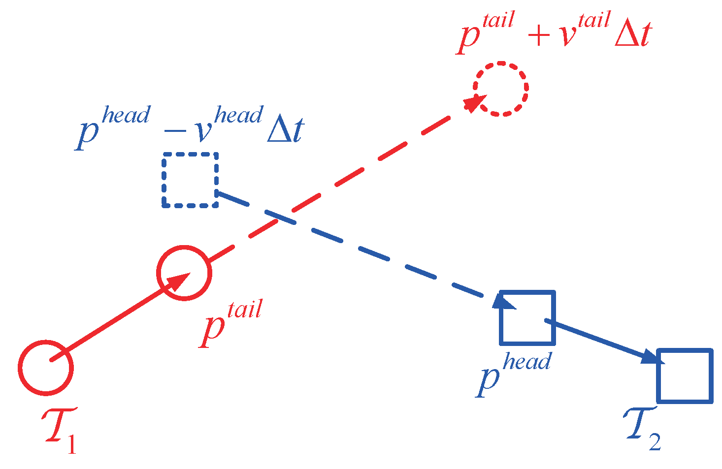
The motion associated probability is defined as

p_{m} (T_{i}^{*} | T_{j}^{*}) = - ln (N (Δ p_{1}, Σ) N (Δ p_{2}, Σ))

(14)

Δ p_{1} = p_{i}^{t a i l} + v_{i}^{t a i l} Δ t - p_{j}^{h e a d}

(15)

Δ p_{2} = p_{j}^{h e a d} - v_{i}^{h e a d} Δ t - p_{i}^{t a i l}

(16)

where

Δ t

denote as the frame gap between the last detections set of the tracklet

T_{j}^{*}

and the first detections set of the tracklet

T_{i}^{*}

p_{i}^{h e a d}

and

p_{i}^{t a i l}

are the center position of the first and last detections set of the tracklet

T_{i}^{*}

, respectively.

v_{i}^{h e a d}

and

v_{i}^{t a i l}

indicate the estimated speed of the tracklet

T_{i}^{*}

at the head and tail, respectively. The motion affinity between two tracklets is shown in Figure 2.

In this case, it is assumed that the error of the predicted location and the central location of the detection set

Δ p_{1}

and

Δ p_{2}

follows a Gaussian distribution. The smaller the error between the predicted position and the actual position of the target to be connected, the greater the motion similarity between the corresponding track slices will be. The temporal associated cost is defined as:

p_{t} (T_{i}^{*} | T_{j}^{*}) = \{\begin{matrix} 1, \\ 0, \end{matrix} \begin{matrix} Δ t \in [1, ς] \\ o t h e r w i s e \end{matrix}

(17)

where

ς

is an upper bound of frame gap. The Initialization probabilities and termination probabilities for each tracklet are set to be

P_{Ψ} (T_{i}^{*}) = P_{t} (T_{j}^{*}) = 1

(18)

Similar to the low-level association, we establish the network flow model based on tracklets to solve the motion cost and time cost between the tracklets, and use the A* search algorithm to obtain the optimal trajectories.

3.3. Trajectory Smoothness

In this section, we use the in-coordinate interval Kalman smoothing algorithm to calculate the extended target’s state. The algorithm consists of forward filtering and backward smoothing. Assume that the interval between two frames is defined as

k (i) = k (0) + i \times T, (i = 0, 1, 2, . . ., M_{l})

, where T is the sampling time. At the time

k (i) (i = 0, 1, 2, . . ., M_{l} - 1)

, the Kalman filter only predict the state of extended target until a new measurement arrives at time

k (M_{l})

, the time update is as follows

s_{k (i) | k (i - 1)} = F_{k (i - 1)} s_{k (i - 1)}

(19)

P_{k (i) | k (i - 1)} = F_{k (i - 1)} P_{k (i - 1)} F_{k (i - 1)}^{T} + w_{k (i)}

(20)

where

s_{k (i)}

denote as the extended target state at the time

k (i)

F_{k (i - 1)}

is the transition matrix. Once the measurements arrived at the time

k (M)

, the forward filtering step is

s_{k (M_{l}) | k (M_{l} - 1)} = F_{k (M_{l} - 1)} s_{k (M_{l} - 1)}

(21)

P_{k (M_{l}) | k (M_{l} - 1)} = F_{k (M_{l} - 1)} P_{k (M_{l} - 1)} F_{k (M_{l} - 1)}^{T} + w_{k (M_{l})}

(22)

K_{k (M_{l})} = P_{k (M_{l}) | k (M_{l} - 1)} H_{k (M_{l})}^{T} {[H_{k (M_{l})} P_{k (M_{l}) ∣ k (M_{l} - 1)} H_{k (M_{l})}^{T} + E_{k (M_{l})}]}^{- 1}

(23)

s_{k (M_{l})} = s_{k (M_{l}) | k (M_{l} - 1)} + K_{k (M_{l})} [{\bar{z}}_{k (M_{l})} - H_{k (M_{l})} s_{k (M_{l}) | k (M_{l} - 1)}]

(24)

P_{k (M_{l})} = [I - K_{k (M_{l})} H_{k (M_{l})}] P_{k (M_{l}) ∣ k (M_{l} - 1)}

(25)

where

{\bar{z}}_{k (M_{l})}

represents the mean of measurements of the extracted extended target at time

k (M_{l})

. Here, the state and covariance matrix at each time are calculated by backward recursive method starting from the last time

k_{m a x}

, given by

s_{k ∣ k} = F_{k} s_{k ∣ k + 1}

(26)

P_{k ∣ k} = F_{k} P_{k ∣ k + 1} F_{k}^{T}

(27)

J_{k} = P_{k ∣ k + 1} F_{k + 1}^{T} P_{k ∣ k + 1}^{- 1}

(28)

s_{k ∣ k_{m a x}} = s_{k ∣ k} + J_{k} (s_{k + 1 ∣ k_{m a x}} - s_{k ∣ k + 1})

(29)

P_{k ∣ k_{m a x}} = P_{k ∣ k} + J_{k} (P_{k + 1 ∣ k_{m a x}} - P_{k ∣ k + 1}) J_{k}^{T}

(30)

where

s_{k ∣ k_{m a x}}

and

P_{k ∣ k_{m a x}}

represent the smoothness state estimation and covariance matrix at time k, respectively.

J_{k}

is the smoothness gain matrix.

4. Experimental Results

Case 1: Numerical simulation

In the simulation, the validity of the ET-HT filter is tested. Consider a 2-D surveillance region which is set as

[3000, 10000] m \times [0, 6000] m

, the clutter intensity

c_{k} = 5 \times 10^{- 17}

. The time steps is set to 30, the sampling period is defined as

T = 1 s

. There are two maneuvering extended targets, and their initial positions are set to

[6000, 4500] m

[3500, 3000] m

, respectively. Their start velocities are set to

[0, - 150] m / s

and

[200, - 20] m / s

. The start time and terminal time in this system are

[1, 5] s

and

[5, 30] s

, respectively. The kinematic state is given by

s_{i, k} = F_{i, k} s_{i, k - 1} + w_{i, k}

(31)

where

s_{i, k} = [x_{i, k}, y_{i, k}, {\dot{x}}_{i, k}, {\dot{y}}_{i, k}]

is the state variable.

x_{i, k}

and

y_{i, k}

represent the location of the targets, respectively.

{\dot{x}}_{i, k}

and

{\dot{y}}_{i, k}

represent the velocity of the targets, respectively.

F_{i, k}

is the kinematic state transition matrix of i-th target.

w_{i, k}

represents the Gaussian process noise of the i-th target with zero mean and covariance

Q_{i, k}

Q_{i, k} = d i a g [100, 100]

The measurement model is defined as

z_{i, k} = H_{k} s_{i, k} + E_{i, k}

(32)

where

H_{k}

is the observation matrix,

z_{i, k}

is defined as the measurements generated by the i-th target at time k,

E_{i, k}

denotes as the Gaussian measurement noise of the i-th target with zero mean and covariance

R_{i, k}

R_{i, k} = d i a g [100, 100]

In the simulation, the clutter poisson rate

λ_{c}

is set to 600, then clutter density

λ_{c} c_{k}

3 \times 10^{- 15}

. The failure and recovery rate are set to

p_{f} = 0.2

q_{s} = 0.8

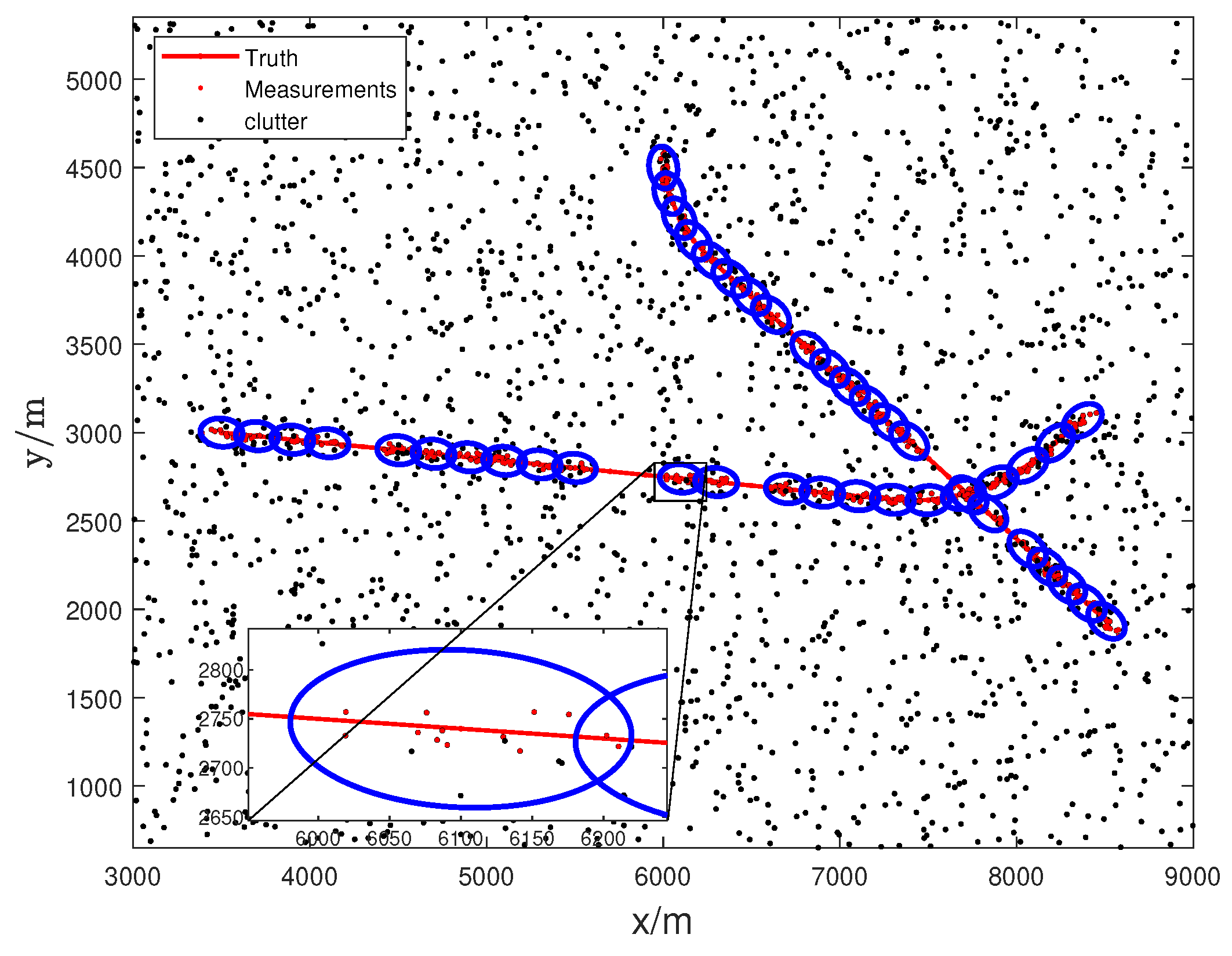
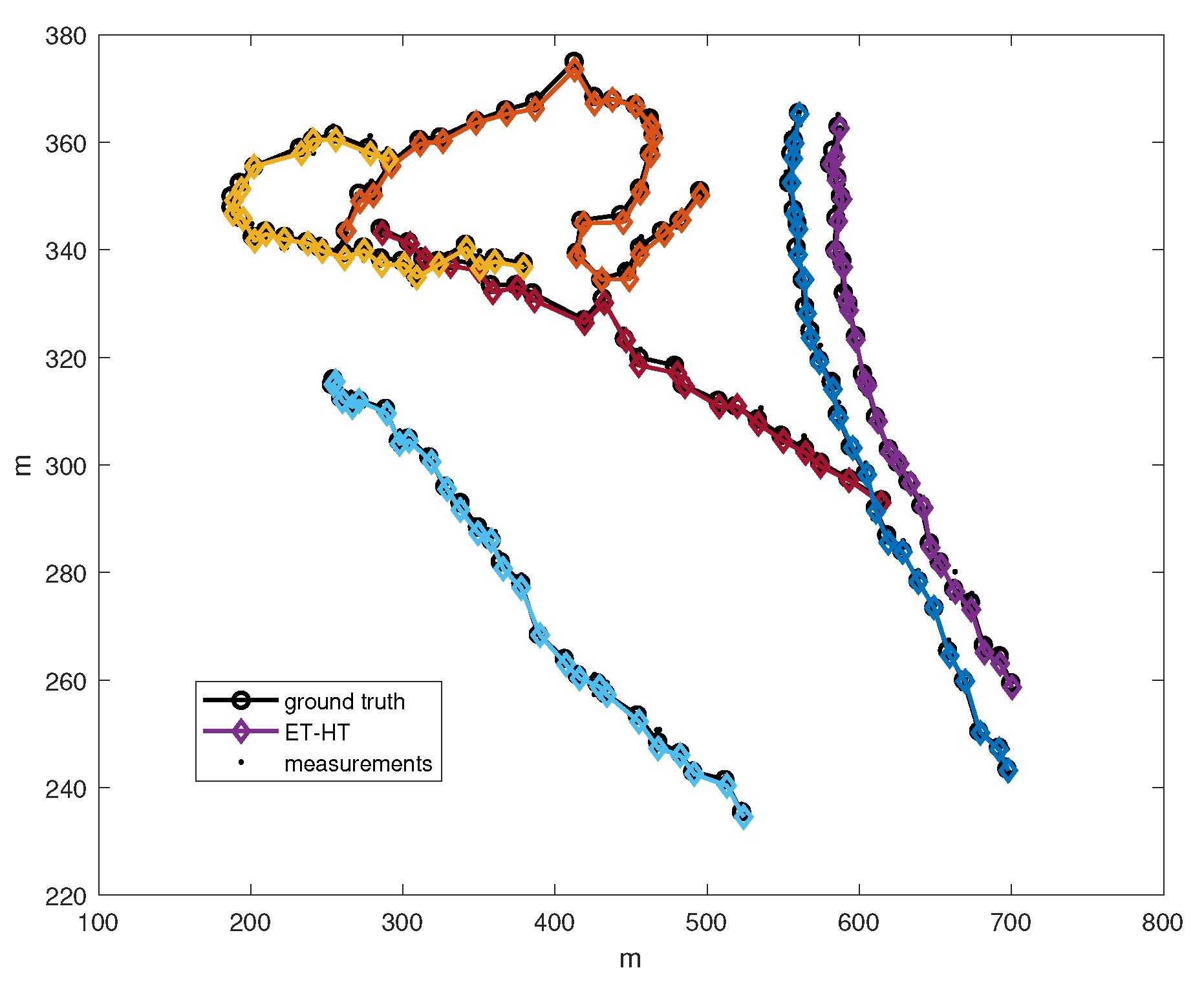
, respectively. The simulated target scenario with intermittent measurements is shown in Figure 3.

In our experiment, we take into account the absolute mean number of targets estimation error (NTE) [24] and the optimal subpattern assignment (OSPA) distance [25] as metrics to evaluate the performance of the proposed ET-HT filter against the ET-GM-PHD, ET-JPDA, and ET-PMBM filters. The absolute mean number of targets estimation error is defined as

N T E (X_{k}, Y_{k}) = E {| X_{k} | - | Y_{k} |}

(33)

where

X_{k}

and

Y_{k}

are two finite subsets,

| X_{k} |

and

| Y_{k} |

represent the potential of the two subsets, respectively. The OSPA distance between

X_{k}

and

Y_{k}

is defined as the distance between the position and the potential of the two sets.

O S P A (p, c, X_{k}, Y_{k}) = {(\frac{1}{n} (min_{π \in \prod_{n}} \sum_{i = 1}^{n} d^{(c)} {(x_{i}, y_{i})}^{p} + c^{p} (m - n)))}^{1 / p}, n \leq m

(34)

where c is the penalty cost for cardinality mismatch, p is the order of the OSPA metric,

1 < p < \infty

c > 0

. In the simulation, they are set to 10 and 2, respectively.

The OSPA distances and NTEs of four filters are depicted in Figure 4. Comparatively, the ET-HT filter exhibits lower OSPA distance and NTE values when compared to the other filters. In contrast, the performance of the ET-JPDA filter is influenced by clutter and necessitates prior knowledge regarding the number of targets. As the estimation error increases, the OSPA distance and NTE of the ET-JPDA filter also escalate. On the other hand, the ET-GM-PHD filter leverages the first-order approximate moment of the multi-target density to convey valuable information about target potential.When the motion trajectories intersect, the targets are partitioned into one cell, which leads to an increase in the OSPA distance. Meanwhile, the ET-GM-PHD and ET-PMBM filters require precise models of both targets and clutter. However, the lack of prior information and the interference of clutter result in a large discrepancy between the estimated and actual number of targets, which incurs the NTE increases.

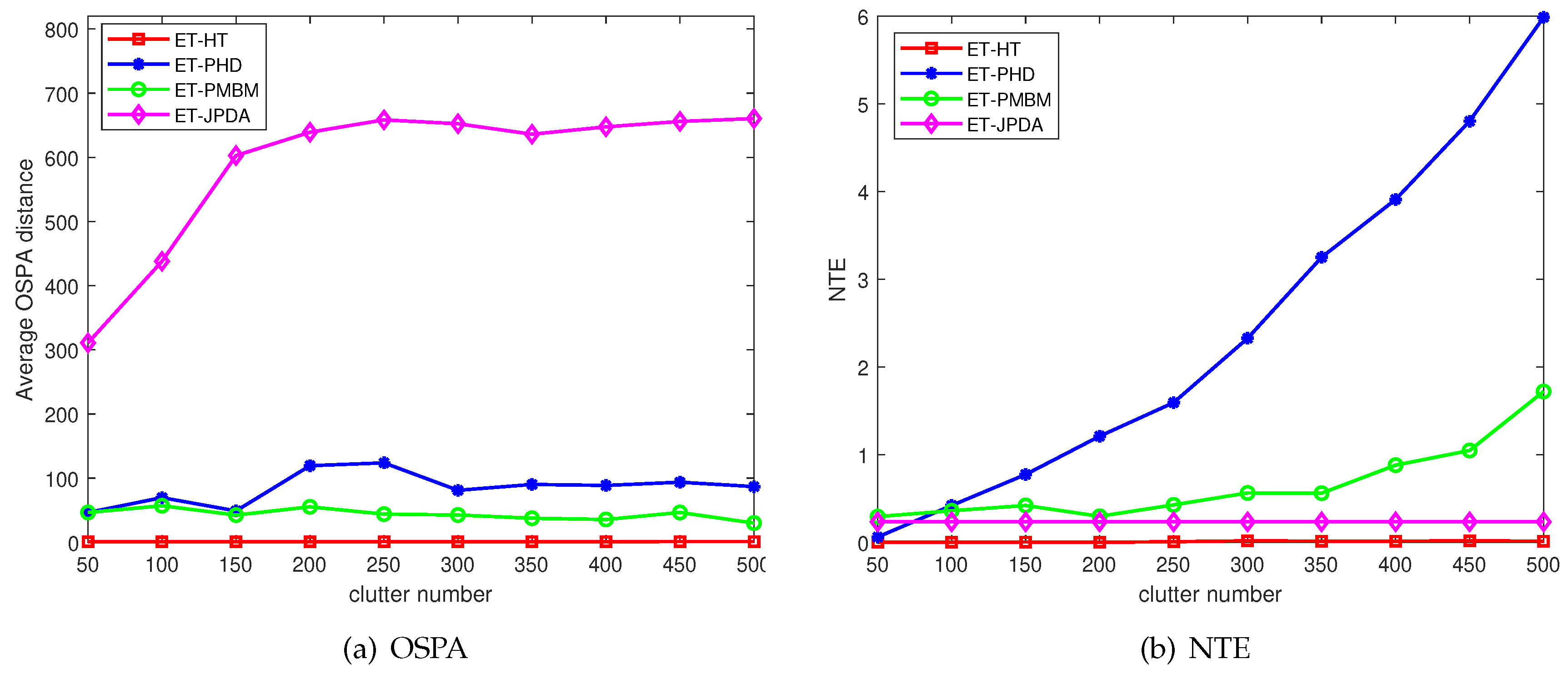
Figure 5 presents the average OSPA distances and NTEs of the four filters at varying clutter rates. The ET-HT filter consistently demonstrates smaller average OSPA distance and NTE compared to the ET-JPDA, ET-PMBM, and ET-GM-PHD filters. To delve further into the influence of intermittent probability, the investigation extends to different failure rate

p_{f}

and recovery rate

q_{s}

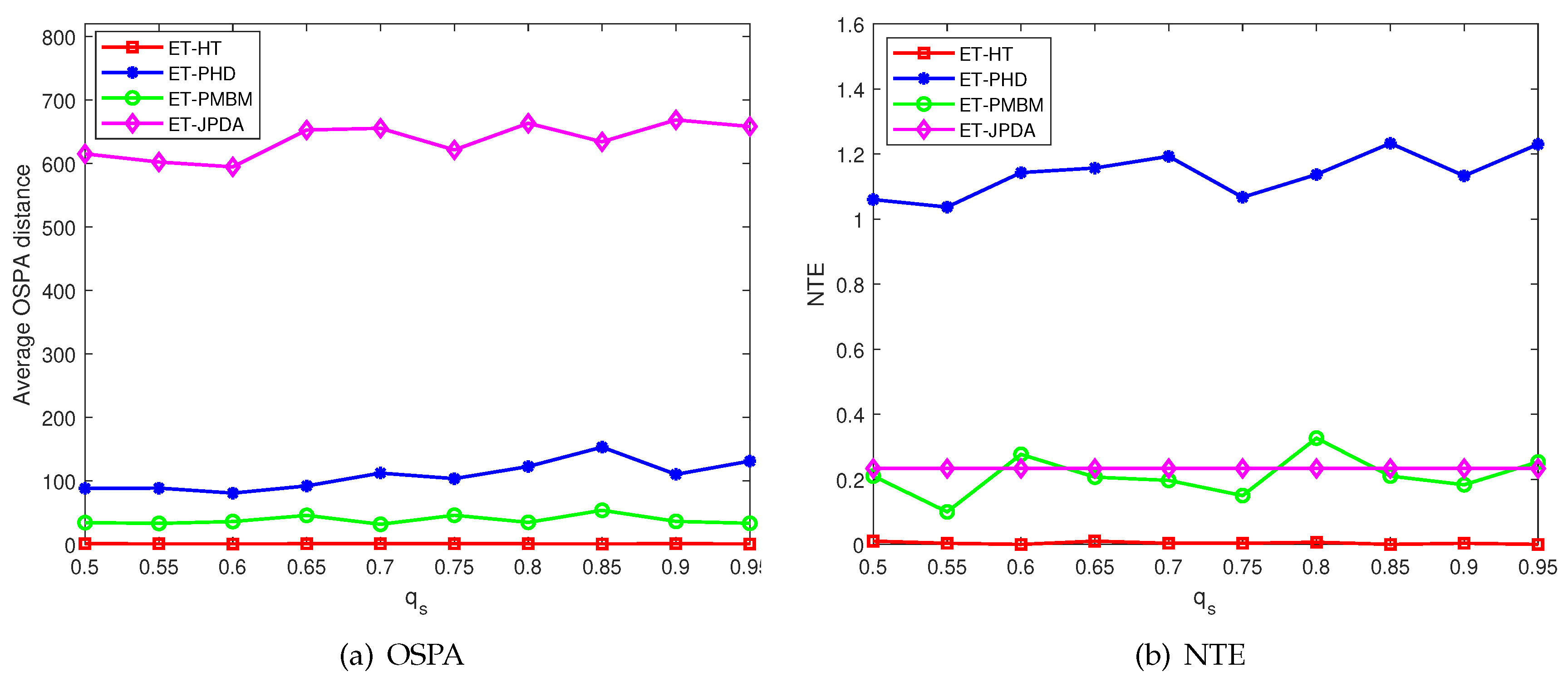
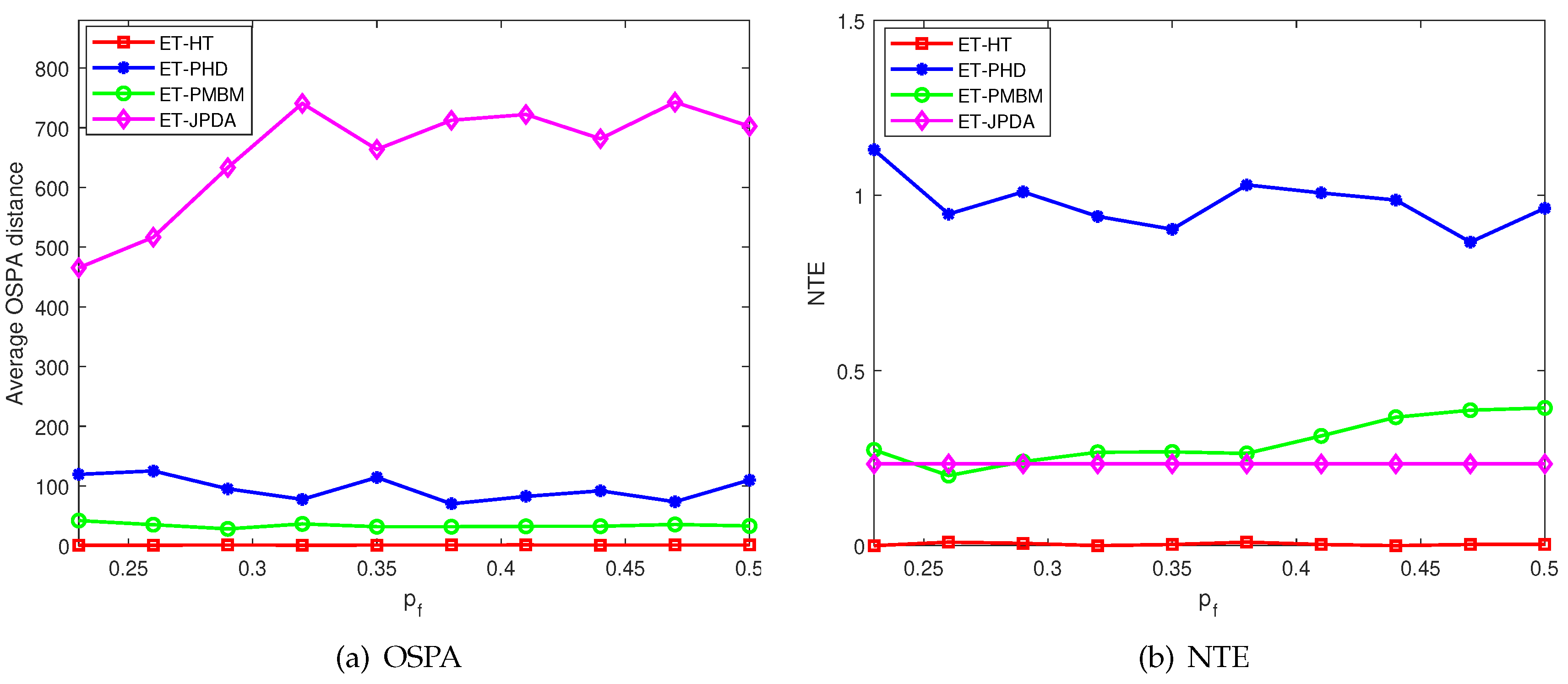
. The OSPA distances and NTEs of the four filters are illustrated in Figure 6(a) and 6(b), respectively, considering diverse recovery rates in 100 Monte Carlo runs. Likewise, Figure 7(a) and 7(b) depict the OSPA distances and NTEs of the filters for varying failure rates with 100 Monte Carlo runs.

The results from Figure 6 and 7 clearly demonstrate that the ET-HT filter exhibits superior tracking performance compared to the ET-GM-PHD, ET-PMBM and ET-JPDA filters irrespective of the transformation of the measurement recovery and loss rates. This is because the ET-HT filter associates the tracklets into long tracks through both low-level and high-level associations, thereby reducing the impact of intermittent measurements.

On the other hand, the results obtained from the ET-JPDA filter suggest that measurement loss can cause a mismatch between the tracking gate and the measurement, resulting in an increase in the OSPA distance. Similarly, the results of the ET-PHD filter indicate that some pieces of clutter are incorrectly identified as targets, leading to errors in estimating the number of targets and an increase in the NTE. Nonetheless, the presence of clutter affects the division of the measurements, and both the ET-PMBM filter’s OSPA distance and NTE are larger than those of the ET-HT filter.

Time Complexity

The time complexity of the ET-HT filter consists of two main components, namely the adaptive spectral clustering algorithm and the worst-case of the search subgraph. The time complexity of the former is

O (n \times (N_{t c} - n_{t c})) + O (n_{t c}^{3}) + O (K_{t c} N_{t c} I_{t c}) \cdot O (n_{t c} \times (N_{t c} - n_{t c}))

, where

K_{t c}

is the number of nodes in the undirected graph,

n_{t c}

is the sample points,

N_{t c}

is the number of trajectories and

I_{t c}

is the iteration number of K-means algorithm. The worst time complexity of searching sub-graph is

O (n_{max}^{2})

[26].

The time complexity of the ET-JPDA filter is

O (N_{t c} \times n_{t c}^{2})

, where

N_{t c}

is the initial number of targets,

n_{t c}

is the sampling time. The time complexity of the ET-PHD filter is

O (N_{t c} \times n_{t c}^{2}) + O (n_{t c} \times M_{t c} \times N_{t c}^{2} \times d_{t c}^{2})

, where the parameter

M_{t c}

is generally greater than 1000, and

d_{t c}

is the dimension of the state vector. The time complexity of the ET-PMBM filter is

O (N_{t c}^{3} \times H_{t c}^{3})

, where

H_{t c}

represents the number of hypothetical combinations. The running times of the four filters for 100 Monte Carlo runs are shown in Table 1.

Case 2 :Real data verification

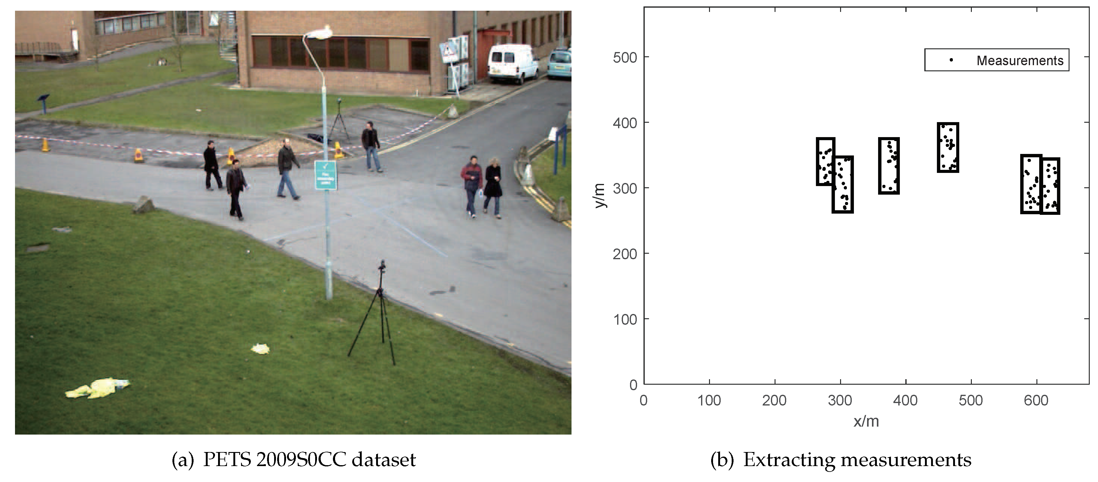
To evaluate the performance of the proposed data association approach, the ET-HT filter framework is applied to a scenario from the PETS 2009S0CC [27] dataset. In this dataset, we focus on a specific scene featuring six pedestrians walking. Their paths intersect at specific frames (295, 305, 345, 365, and 367). Additionally, in frames 319, 339, and 351, the pedestrians are obstructed by a street light, as illustrated in Figure 8(a). Figure 8(b) shows the extracted measurements.

We used MatlabR2019b, which is based on an Intel CPU i74770k 3.5 GHz, DDR3 32 GB RAM, to implement the proposed ET-HT filter, and tested it on 768 x 576 frames. The results of the extended target tracking are shown in Figure 9.

The real data verification has successfully demonstrated the effectiveness of our proposed ET-HT filter, which is able to accurately correlate targets with intermittent measurements using the ET-HT filter.

5. Conclusion

This paper proposed a Hierarchical Network-based Tracklets Data Association algorithm, which can be used in the field of multiple extended target tracking with intermittent measurements. The low-level extracts all possible tracklets, which are then used to construct a network flow model. A * search algorithm is used to compute the trajectories of multi-extended targets. Simulation results show that the ET-HT filter significantly outperforms traditional data association algorithms, and its performance is unaffected by clutter parameters and intermittent probability. In the future, we plan to consider observation delay and embed it into multi-object trackers, as well as multi-sensor estimation.

Author Contributions

Kaiyi Jiang and Tianli Ma conceived and designed the algorithm; Kaiyi Jiang performed the experiments, analyzed the data, and drafted the paper; Lin Li and YiGuo Li revised the manuscript.

Funding

This work was supported in part by the National Natural Science Foundation of China, grant number 82101969, in part by the Regional Innovation Capability Guidance Program Project of Shaan xi Province, grant number 2022QFY01-16, in part by the Key Research and Development Project of Shaan xi Province, grant number 2022GY-242, and in part by the Science and Technology Plan Project of Xian Yang City, grant number 2021ZDYF-SF-0020.

Conflicts of Interest

The authors declare no conflict of interest.

References

Mahler R, P. Advances in statistical multisource-multitarget information fusion. Journal Abbreviation 2008, 10, 142–149. [Google Scholar]
Lan J, Li X R. Tracking of extended object or target group using random matrix: new model and approach. In IEEE Transactions on Aerospace & Electronic Systems; 2016, 52(6), 2973-2989.
Morelande M R, Kreucher C M, Kastella K. A Bayesian Approach to Multiple Target Detection and Tracking. In IEEE Transactions on Signal Processing; 2007, 55, 1589–1604.
Vivone G, Braca P. Joint Probabilistic Data Association Tracker for Extended Target Tracking Applied to X-Band Marine Radar Data. In IEEE Journal of Oceanic Engineering; 2016, 41(4), 1007-1019.
Habtemariam B, Tharmarasa R, Thayaparan T. A Multiple-Detection Joint Probabilistic Data Association Filter. In IEEE Journal of Selected Topics in Signal Processing; 2013, 7(3), 461-471.
Schuster M, Reuter J, Wanielik G. Multi- detection joint integrated probabilistic data association using random matrices with applications to radar-based multi object tracking. In IEEE Journal of Advances in Information Fusion; 2013, 12(2), 175-188.
Xie Y, Huang Y, Song T L. Iterative joint integrated probabilistic data association filter for multiple-detection multiple-target tracking. In Digital Signal Processing; 2018, 72, 232–243.
Yang S, Wolf L M, Baum M. Marginal Association Probabilities for Multiple Extended Objects without Enumeration of Measurement Partitions. In 2020 IEEE 23rd International Conference on Information Fusion; 2020, 1-8.
Peng L, Ge H W, Yang J L, et al. Modified Gaussian inverse Wishart PHD filter for tracking multiple non-ellipsoidal extended targets. In Signal Processing; 2018, 150, 191–203.
Peng M S, Linares R, Bageshwar V L. Extended Target Tracking and Shape Estimation via Random Finite Sets. In 2019 American Control Conference; 2019, 72, 232–243.
Zou Z B, Song L P. Labeled box-particle CPHD filter for multiple extended targets tracking. In Journal of Systems Engineering & Electronics; 2019, 3, 1–8.
Liang Z, Liu F, Li L. Improved generalized labeled multi-Bernoulli filter for non-ellipsoidal extended targets or group targets tracking based on random sub-matrices. In Digital Signal Processing; 2020, 99, 102669–102682.
Granstrom K, Svensson L, Reuter S. Likelihood-Based Data Association for Extended Object Tracking Using Sampling Methods. In IEEE Transactions on Intelligent Vehicles; 2018, 2, 1–14.
Su Z Z, Ji H B, Zhang Y. Data association for extended target tracking by BP. In IET Radar, Sonar & Navigation; 2018, 12(12), 1484-1492.
Su Z Z, Ji H B, Zhang Y. Loopy belief propagation based data association for extended target tracking. In Chinese Journal of Aeronautics; 2020, 33(8), 2212-2223.
Yazdian D M, Azimifar Z. An improvement on GM-PHD filter for target tracking in presence of subsequent miss-detection. In 2015 23rd Iranian Conference on Electrical Engineering; 2015.
Ma T L, Wang X M, Li T. Multiple-model multiple hypothesis probability hypothesis density filter with blind zone. In International Journal of Industrial & Systems Engineering; 2017, 27(2), 180-195.
Wu W, Sun H, Cai Y. Tracking multiple maneuvering targets hidden in the DBZ based on the MM-GLMB filter. In IEEE Transactions on Signal Processing; 2020, 99, 1–12.
You K Y, Fu M Y, Xie L H. Mean Square Stability for Kalman Filtering with Markovian Packet Losses. In Automatica; 2011, 47, 1247–1257.
Guo P, Liu Z, Wang J J. HRRP multi-target recognition in a beam using prior-independent DBSCAN clustering algorithm. In IET Radar, Sonar & Navigation; 2019, 13(8), 1366-1372.
Xi Z, Liu H. Multiple Object Tracking Using the Shortest Path Faster Association Algorithm. In The scientific world journal; 2014, 2014, 481719–481730.
Särkkä, S. Schuhmacher D. Continuous-time and continuous-discrete-time unscented Rauch–Tung–Striebel smoothers. Signal Process. 2010, 90, 225–235. [Google Scholar]
Huang, Y.; Zhang, Y.; Zhao, Y.; Mihaylova, L.; Chambers, J. A Novel Robust Rauch–Tung–Striebel Smoother Based on Slash and Generalized Hyperbolic Skew Student’s T-Distributions. In Proceedings of the 2018 21st International Conference on Information Fusion (FUSION), Cambridge, UK, 10–13 July 2018; pp. 369–376. [Google Scholar]
Wang Y, Meng H, Liu Y, et al. Collaborative penalized Gaussian mixture PHD tracker for close target tracking [J]. Signal Processing, 2014, 102: 1-15.
Särkkä, S.Schuhmacher D, Vo B T, Vo B N. A consistent metric for performance evaluation of multi-object filters[J]. IEEE Transactions on Signal Processing, 2008, 56(8): 3447 - 3457.
Ma T, Gao S, Chen C, Song X. Multitarget Tracking Algorithm Based on Adaptive Network Graph Segmentation in the Presence of Measurement Origin Uncertainty. Sensors. 2018; 18(11):3791.
IEEE International Workshop on Performance Evaluation of Tracking and Surveillance (PETS) 2009 Dataset.

Figure 1. The flow chart of Hierarchical network-based tracklets data association for multiple extended targets tracking with intermittent measurements.

Figure 2. The motion affinity between two tracklets.

Figure 3. Target trajectories and measurements.

Figure 4. The average OSPA distance and NTE of a single example run, with

q_{s} = 0.8

p_{f} = 0.2

λ_{C} = 300

Figure 4. The average OSPA distance and NTE of a single example run, with

q_{s} = 0.8

p_{f} = 0.2

λ_{C} = 300

Figure 5. The average OSPA distance and NTE for 100 Monte Carlo runs, with

q_{s} = 0.8

p_{f} = 0.2

Figure 5. The average OSPA distance and NTE for 100 Monte Carlo runs, with

q_{s} = 0.8

p_{f} = 0.2

Figure 6. The average OSPA distances and NTE of different recovery rates for 100 Monte Carlo runs, with

p_{f} = 0.2

λ_{C} = 600

Figure 6. The average OSPA distances and NTE of different recovery rates for 100 Monte Carlo runs, with

p_{f} = 0.2

λ_{C} = 600

Figure 7. The average OSPA distances and NTE of different failure rates for 100 Monte Carlo runs, with

q_{s} = 0.8

λ_{C} = 600

Figure 7. The average OSPA distances and NTE of different failure rates for 100 Monte Carlo runs, with

q_{s} = 0.8

λ_{C} = 600

Figure 8. An example of the PETS2009S0CC dataset. We input the extracted measurement points into the ET-HT filter. After hierarchical clustering, these measurement points can be regarded as pedestrian motion trajectories.

Figure 9. The tracking results by the ET-HT filter.

Table 1. Average running time of four filters.

Filter	ET-HT	ET-PHD	ET-PMBM	ET-JPDA
Time(t/s)	10.1369	2232.9	96.3917	1.1254

Disclaimer/Publisher’s Note: The statements, opinions and data contained in all publications are solely those of the individual author(s) and contributor(s) and not of MDPI and/or the editor(s). MDPI and/or the editor(s) disclaim responsibility for any injury to people or property resulting from any ideas, methods, instructions or products referred to in the content.

© 2023 by the authors. Licensee MDPI, Basel, Switzerland. This article is an open access article distributed under the terms and conditions of the Creative Commons Attribution (CC BY) license (http://creativecommons.org/licenses/by/4.0/).

Copyright: This open access article is published under a Creative Commons CC BY 4.0 license, which permit the free download, distribution, and reuse, provided that the author and preprint are cited in any reuse.

MDPI Initiatives

Important Links

Choose an area of interest and we will send you notifications of new preprints at your preferred frequency.

Disclaimer

Hierarchical Network-Based Tracklets Data Association for Multiple Extended Targets Tracking With Intermittent Measurements

Abstract

1. Introduction

2. Problem Formulations

3. Hierarchical Network-Based Data Association for Multiple Extended Target Tracking

3.1. Pre-Processing

3.2. Hierarchical Association

a. low-level association network

b. high-level association network

3.3. Trajectory Smoothness

4. Experimental Results

Case 1: Numerical simulation

Time Complexity

Case 2 :Real data verification

5. Conclusion

Author Contributions

Funding

Conflicts of Interest

References

MDPI Initiatives

Important Links

Subscribe