
Submitted:
19 May 2023
Posted:
22 May 2023
You are already at the latest version
Abstract
We prove that the Legendre coefficients associated with a function f(x) can be represented as the Fourier coefficients of a suitable Abel-type transform of the function itself. Thus, the computation of N Legendre coefficients can be performed efficiently in O(NlogN) operations by means of a single Fast Fourier Transform of the Abel-type transform of f(x). We also show how the symmetries associated with the Abel-type transform can be exploited to further reduce the computational complexity. The dual problem of calculating the sum of Legendre expansions is also considered. We prove that a Legendre series can be written as the Abel transform of a suitable Fourier series. This fact allows us to state an efficient algorithm for the evaluation of Legendre expansions. Finally, numerical tests are presented to exemplify and confirm the theoretical results.
Keywords:
Legendre coefficients
; Fourier coefficients
; Legendre expansion
; Abel transform
MSC: 42C10; 44A05; 65R10; 65T50
1. Introduction
The computation of the coefficients of Legendre expansions is a very important problem in numerical analysis and applied mathematics with a wide range of applications including, just to mention a few, approximation theory [1], special function theory [2], spectral methods for differential equations [3] and construction of quadrature formulae [3,4]. Its importance has emerged also in connection with the computation of spectra of highly oscillatory Fredholm integral operators, which play an important role in laser engineering [5]. For its relevance, this problem attracted a significant reserach attention since the Seventies [6,7].
The difficulty of the problem lies essentially in the fact that these coefficients are represented by integrals whose integrands oscillate rapidly for large values of the index of the polynomial. Standard quadrature procedures for the calculation of N Legendre coefficients lead only to slow algorithms (see, e.g., Ref. [6,8]). The first contribution for a more efficient computation of Legendre coefficients traces back to the work of Orszag [9], where the algorithm uses a slowly converging first-order WKB expansion of the Legendre polynomials.
More efficiently, in Ref. [10] the Legendre coefficients are obtained by transforming the corresponding Chebyshev coefficients through a multipole-like expansion, which yields a fast algorithm, though requiring a considerable and rather expensive initialization phase. In this context, various improvements have been proposed, e.g., in [11,12]. Remaining within this kind of approach, [13] describes an Chebyshev-Legendre transform, which is based on the Stieltjes’ asymptotic formula for the Legendre polynomials of large degree. Mori et al. [14] employed the same asymptotic formula to produce a fast algorithm but affected by a problem of numerical instability for large N. The connection between Legendre and Chebyshev coefficients is analyzed also in [15] in the case of piecewise smooth functions. In Ref. [16] (see also [17]) an algorithm is given, for N a power of two, which requires a suitably preprocessed data structure.
Another way to tackle this problem has been described in [18], where an algorithm for the rapid computation of the Legendre coefficients is presented when the analytic expression of the input function is known on a Bernstein ellipse in the complex plane. The algorithm has complexity but requires the knowledge of the region of analyticity of the function in .
In this paper we present an alternative procedure. The basic idea of our method consists in exploiting the Dirichlet-Murphy integral representation of the Legendre polynomials. We prove that the coefficients of the Legendre expansion of a function are connected with a subset of the Fourier coefficients (the ones with nonnegative index) of an Abel-type transform of .
The numerical implementation of the algorithm follows straightforwardly and is very efficient. The aforementioned Fourier coefficients (which represent the sought for Legendre coefficients) can be computed in operations by a single Fast Fourier Transform (FFT) after the evaluation of the Abel-type integral by means of standard quadrature techniques.
The dual problem of calculating the values of (finite) Legendre expansions is analyzed in Section 3. In SubSection 3.1 we prove that the Legendre expansions can be computed by means of a (inverse) cosine transform of a sequence of coefficients, which is obtained by a suitable linear transformation of the given set of N Legendre coefficients. Further, a novel algorithm is presented in SubSection 3.2, where the Legendre expansions are proved to be the Abel-type transform of a Fourier series, the coefficients of the latter being the Legendre coefficients of the function . This leads to an efficient algorithm which requires the computation of one FFT and of one Abel-type integral.
2. Connection between Legendre expansions and Fourier series
The standard form of the Legendre expansion reads:
where are the Legendre polynomials, which can be defined by the generating function [19]:
and the coefficients are given by:
The conditions to be satisfied by to guarantee the uniform convergence of the series in (1) will be discussed in the next section. However, for our current purpose of computing the Legendre coefficients , it is sufficient to assume that be absolutely integrable on the interval . For later convenience, we define the normalized Legendre coefficients as
We can now state the following theorem.
Theorem 1.
The normalized Legendre coefficients coincide with the Fourier coefficients, with , of an Abel-type transform of , that is:
where the -periodic function is defined by
being the sign function.
Proof.
We consider the Dirichlet-Murphy integral representation of the Legendre polynomials [20](Ch. III, §5.4):
Interchanging the order of integration in (8) we obtain:
Next, if we make the change of variables: and , the second integral on the r.h.s. of (9) becomes:
It is easy to check from (6) that satisfies the following symmetry relation:
which, in view of (5), induces the following symmetry on the coefficients :
2.1. Numerical issues
Let us now consider the actual problem of computing the first N Legendre coefficients (or, equivalently, Nnormalized coefficients ) associated with the function (see (1) and (3)).
The numerical implementation of the algorithm suggested by Theorem 1 requires the computation of the Fourier coefficients (5) of the Abel-type integral function defined in (6). For what concerns the computation of , the integrand presents a weak algebraic singularity at the end point of the domain of integration, which can be effectively handled by means of a proper nonlinear change of variable. This technique, along with the use of a standard quadrature formula (e.g., the Gauss-Legendre one), allows obtaining high accuracy with a small number of nodes [21]. Quadrature formulae suited to end-point singular integrands can also be used [22,23].
It is ought to stress that the function does not depend on the order n of the Legendre polynomial. Therefore, the computational cost for evaluating is independent of the number N of Legendre coefficients to be computed. This means that the number of knots which are necessary to compute the integral in (with a prescribed fixed accuracy ) does not depend on N, but depends only upon the oscillatory characteristics of the function (i.e., the number of samples needed to determine uniquely) and on the accuracy . The oscillatory contributions due to the Legendre polynomials or, in other words, the dependence on the order n of the Legendre polynomial, are accounted for only in the Fourier formula (5) and are neatly separated from the oscillatory contributions ascribable to the input function . The consequence of this decoupling is the low computational complexity of the whole algorithm. In fact, formula (5) makes it possible to take full advantage of the computational efficiency of the Fast Fourier Transform both in terms of speed of computation and of accuracy [24,25]. The first N Fourier coefficients of (which coincide with the normalized Legendre coefficients of ) can thus be computed by a single FFT from the values (samples) of at N distinct points in time. As we have seen above, the number of operations for the calculation of each sample of is independent of N and, consequently, the (asymptotic) computational complexity of the entire algorithm for the computation of the Legendre coefficients coincides with that of the FFT, i.e., . Moreover, in view of the symmetry relation (13), the number of calls to the procedure for the computation of the Abel integral is halved. Of course, if samples are needed to determine uniquely the function and we want the error to be as small as possible, then all the samples of must be used for the numerical computation of the Abel integral and, consequently, the total number of operations in the algorithm will be . Therefore, following logical lines similar to those adopted by Alpert and Rokhlin in Ref. [1] (and, more generally, in methods like, e.g., the Fast Multipole Methods [26]), the reduction of complexity from to is obtained by accepting a lower precision in the computation (in our case, a lower precision in the computation of the Abel integral).
We want to remark two additional features of the algorithm just presented. First, the algorithm does not require the knowledge of the input function at a specific and prescribed set of knots (see, for instance, Ref. [10] where the input function is supposed to be known at Chebyshev knots). The function enters the algorithm only through its Abel-type integral. This allows a significant flexibility in choosing the quadrature scheme which is more suitable for the distribution of knots at which the input function is known (e.g., uniform grid, Chebyshev grid, set of measurements of non-uniformly distributed).
The final remark concerns the robustness of the algorithm against the noise. In the case the values of are only approximately known, e.g., when the input samples of represent measurements affected by error, the effects of the noise in the calculation of the coefficients are damped by the algorithm. In fact, the noisy input samples of are smoothed by the Abel integral operator [27] before being analyzed (encoded as samples of ) by the oscillatory Fourier integral (5).
The procedure described above has been implemented in double precision arithmetics using the standard open source GNU Scientific Library (GSL) [28]. Feasibility and accuracy of the algorithm have been verified by direct comparison of the obtained numerical results with the true Legendre coefficients for a variety of functions. Hereafter we report some of them.
Table 1 displays the absolute error in the computation of Legendre coefficients for four functions with different degree of regularity: the discontinuous function (with being the sign function and a constant), whose Legendre coefficients are , for ; the function: , whose Legendre coefficients are [3](p. 78):
the function with (with a singlarity for x outside the interval , see (2)); the -analytic function: with ( denoting the Bessel function of the first kind and zeroth order).
The first observation from Table 1 is that the accuracy depends on the degree of smoothness of the function because of the computation of the Abel transform of that, in order to obtain a given target precision, requires more quadrature knots for low regular functions. For what concerns the smooth (within the interval ) functions and , which give similar results, the accuracy increases significantly to reach values comparable with the -machine.
The algorithm sources of error are: the approximation of integral (5) by the Discrete Fourier Transform; the approximation of the Abel transform (6) by quadratures and, finally, the finite accuracy of the floating-point arithmetic. The first source of error is ruled by N. This is clearly visible from Figure 1(A), where the maximum error is plotted versus N. For the -function (asterisks), we see that for low values of N the maximum error is mainly ascribable to the error due to the approximation of the Fourier integral with the DFT and to the approximation of the Abel integral: it decreases like up to , and then starts increasing like , as in the case of smooth functions. From the comparison with the plot of maximum error for smooth functions (triangles), we can also say that the number of points N used in the DFT need not to be unnecessary large unless the function itself has low regularity.
The computation of N Legendre coefficients by ordinary quadrature produces an algorithm. The increment of performances of the algorithm presented here has been verified by evaluating the speed of computation at (nearly) same precision. The results of these tests are illustrated in Figure 1(B), where the execution time T (in seconds) is plotted versus the number N of computed Legendre coefficients. The results show an execution time (at least in the N-interval we considered, up to ) independently of the regularity properties of the input function , confirming the expected great increase of computational speed (asymptotically, the awaited improvement ratio being proportional to ). Such an increase of performances will become even more crucial for the efficient evaluation of multivariate Legendre transform [5] and of spherical harmonic expansions [30], which will be the subject of a forthcoming paper.
3. Computation of Legendre expansions
Let us now move on to consider the problem of evaluating the function from the set of Legendre coefficients . In general, in the complex plane the domain of convergence of the Legendre expansion (1) is the maximal ellipse with foci at within which the function f is analytic [31]. This rather restricted class of functions can be greatly enlarged when we limit ourselves to consider convergence issues on the segment . In Ref. [32] W. H. Young showed the tight connection between Legendre series and Fourier series when . In particular, he proved that in any internal closed interval of the series of Legendre (1) behaves in respect to convergence, divergence, or oscillation, uniform or otherwise, precisely like the Fourier series of where , provided the terms of series (1) are such that
the latter being the natural necessary condition for the convergence of the series (1). More explicitly, e.g., E. W. Hobson [33] provided a test of convergence stating that if the condition
is satisfied (the latter condition being equivalent to require that be integrable on ), then the series (1) is convergent for any near which f is of bounded variation. Since the points are singular points of Legendre’s equation, the convergence at the end points of the interval requires somehow more stringent (than in the Fourier case) conditions such as, e.g., being of bounded variation over the entire interval .
This parallelism between Legendre and Fourier expansions have been already exploited in the previous section where we proved that the (normalized) Legendre coefficients of coincide with the Fourier coefficients of the function . In the next two subsections we continue our analysis along this line, and present two algorithms for the computation of values of Legendre expansions.
3.1. An algorithm for the evaluation of Legendre series
In the theorem that follows we will prove that a Legendre expansion can be computed by calculating the (inverse) cosine transform of a sequence which is obtained by a suitable linear transformation of the set of Legendre coefficients .
Theorem 2.
Let be the function given in (1). Assume that is such that the Legendre expansion (1) and the Fourier expansion of converge uniformly on and , respectively. Then , , can be written as follows:
the coefficients () being given by:
denoting the Legendre coefficients associated with (see (3)) and
Proof.
Since is compactly supported on , the function () is a -periodic function of u. Then, the latter can be represented as the Fourier series,
In view of the uniform convergence of the two series, from (1) and (21) we have:
so that, multiplying both sides of (22) by and integrating on , we have:
The term in the parenthesis on the l.h.s. of (23) is the integral representation of the Kronecker delta . Then, from (23) we have:
with defined in (20). Finally, expansion (18) follows readily by observing that . □
It is worth remarking that the transformation , which connects the Legendre coefficients of with the Fourier coefficients of , is independent of , can be computed with arbitrary precision, and can be regarded as known. In the next proposition we list some known facts on the structure of the matrix K, we give the analytic expression of its entries as smooth function of the indexes (see Ref. [10]), and provide an iterative procedure for computing its elements.
Proposition 1.(i) The coefficients (defined in (20)) can be written as follows:
denoting the Chebyshev polynomials of the first kind.
(ii) The matrix K is upper triangular, and its entries can be computed as follows:
where
denoting the Euler gamma function.
(iii) The following recurrence relation holds for and :
(iv) The diagonal elements can be written as follows:
(v) The elements of the first row can be written as follows:
Proof.
Formula (25) follows from definition (20) by making the substitution into the integral and recalling the definition of the Chebyshev polynomials of the first kind: , (). Representation (ii) of the coefficients is well-known, and it is given, e.g., by Alpert and Rokhlin in [10](formula (20)) (where the matrix K is there named M). The recurrence relation (28) follows from representation (26) and from the following three-term recurrence relations holding, respectively, for the Legendre polynomials and for Chebyshev polynomials :
and
The algorithmic prescription provided by Theorem 2 for the computation of the values of a Legendre expansion is indeed very simple. It consists of a two-step procedure:
- From the N-vector of Legendre coefficients compute the N-vector by , where the (known) upper triangular matrix is defined in (20) (see also Proposition 1);
- Compute the cosine transform of length N of the vector to obtain values of at N selected points of the interval .
The second step of the algorithm presents no difficulties. It is fast since it can be implemented by a single FFT of length N, which requires operations. The standard FFT procedure provides the output on a uniform grid of , so that, according to formula (18), the final result consists of the set of function values at Chebyshev points.
The first step of the algorithm presents instead some aspects which deserve a few comments. The crux is that the matrix is dense and the direct calculation of the matrix-vector product requires operations (precisely, multiplications). Therefore, this step can become a bottleneck for the algorithm when N becomes large. In some practical cases the question is not critical, e.g., when the triangular structure of can be exploited on some computer architectures (e.g., vector machines, parallel GPU) to drop significantly the complexity of the computation. Nevertheless, the reduction of the algorithmic complexity remains an issue. Approximate methods are the only tools to handle effectively the fast computation of the matrix-vector product when the matrix is not structured (i.e., when its entries depend only on parameters). The key to many of these fast methods is renouncing to exactness and accepting the result of the computation within an a-priori fixed level of accuracy. This allows for using approximations of the kernel K which, combined with a suitable subdivision of the matrix into panels, can reduce enormously the cost of computing. Among these algorithms it is worth citing the celebrated Fast Multipole Methods by L. Greengard and V. Rokhlin for the fast evaluation of N-body interactions [12,26,34], which are able to reduce the number of operations to (or even , depending on the matrix structure).
The specific problem we are dealing with here, that is, the fast computation of the matrix-vector product (with given by formula (25)) has been solved brilliantly by B. Alpert and V. Rokhlin in Ref. [10]. In that paper the matrix is first properly divided in square submatrices, and then the computation associated with each submatrix is performed efficiently approximating each entry of the submatrix by its finite Chebyshev expansion. The computational cost brought by a submatrix is then reduced from order of the naive computation to , being the fixed precision required in the Chebyshev interpolation of the submatrix entries. This basic building block allows thus constructing an algorithm for the fast computation of the matrix-vector product with order of complexity.
3.2. A novel algorithm
In this subsection we present a novel algorithm for the inversion of the Legendre transform, which somewhat represents the natural dual algorithm of the one presented in Section 2 for the computation of the forward Legendre transform. In the next theorem we will show that a Legendre expansion can be represented as the Abel-type transform of a suitable Fourier series, the coefficients of the latter being the Legendre coefficients of (cf. Theorem 1).
Theorem 3.
Let be the function given in (1). Assume that is such that the Legendre expansion (1) converges uniformly on . Then , , can be written as follows:
where the function is defined by
denoting the Legendre coefficients associated with (see (3)).
Proof.
First we show that the following integral representation holds for the Legendre polynomials :
Formula (37) can be easily obtained from the Dirichlet-Murphy representation (7) by first splitting the interval of integration into two subintervals: , and then changing the integration variable in the second integral, i.e., we have:
Theorem 3 suggests the following algorithm for the computation of the values of a Legendre expansion:
The first step is fast: the set of values of the function at N equidistant nodes of the interval can be calculated in time by a single FFT.
For what concerns the second step, it should first be noted that the distribution of the nodes is not constrained and, therefore, we are free to calculate at any set of points of the interval by means of formula (42).
The numerical computation of the Abel-type integral in (42), which presents a weak singularity at the left end-point (see also Section 2), is constrained by the fact that the integrand is known only on a uniform grid of the interval (see Step (1) of the algorithm) and, consequently, only quadrature formulae based on equally spaced knots can be used.
In general, the computation of at N points requires operations since the second step of the algorithm requires operations when all the N known values of the function are used for the computation of the integral in (42). However, it is ought to note that for this computation it is not always necessary to implement a full N-knot quadrature procedure, in particular when N is large. The integral in (42) can usually be computed with an a-priori fixed precision by using much less (than N) quadrature knots, the number of knots depending on the implemented quadrature scheme and on the oscillatory characteristics of the integrand, which, ultimately, depend on the oscillatory characteristics of . An instance of a suitable quadrature scheme is given in Refs. [22,23], where quadratures rules are proposed, based on corrections to the trapezoidal rule, for integrands with end-point singularities of various types, including singularities of the form , . The convergence rate of these quadrature formulae is proved to be at least (that is, the approximation error is of the order of ) where denotes the order of the corrected quadrature rule [22,23]. Thus, in these cases and for N sufficiently large, the algorithm we propose for the evaluation of the Legendre expansion becomes convenient in terms of complexity since the number of operations of the second step is a constant independent of N and, for large values of N, the complexity of the entire algorithm will be dominated by the complexity of the FFT used in Step (1).
4. Conclusions
In summary, we have presented a new and fast, i.e., , algorithm for the computation of the coefficients of Legendre expansions. The algorithm is very simple to implement and computes the Legendre coefficients with just a single FFT of an Abel-type transform of the input function. This algorithm calls up a number of natural generalizations to other polynomials systems, for instance, associated Legendre polynomials and the related spherical harmonic expansions.
The dual problem of evaluating a Legendre expansion has been also considered, and two algorithms have been proposed. In the first algorithm the values of the expansion at appropriately chosen points of the interval are computed by simply performing a single (inverse) FFT of a sequence of coefficients, which are obtained by a suitable linear transformation of the given set of N Legendre coefficients. The rapid evaluation of the expansion values requires using approximate methods for the fast calculation of the matrix-vector product. The second algorithm for the calculation of values of Legendre expansions is novel and somehow inverts the logical steps of the algorithm we have proposed for the computation of the Legendre coefficients: the N-term Legendre expansion can be evaluated efficiently (for N sufficiently large) at any point of the interval by computing the Abel-type transform of a suitable Fourier series.
Funding
This research received no external funding.
Institutional Review Board Statement
Not applicable.
Informed Consent Statement
Not applicable.
Data Availability Statement
Not applicable.
Acknowledgments
The author heartily acknowledges many illuminating discussions had with the friend and collegue Giovanni Alberto Viano.
Conflicts of Interest
The authors declare no conflict of interest.
References
- Cheney, C.W. Introduction to Approximation Theory; McGraw-Hill: New York, NY, USA, 1966. [Google Scholar]
- Rainville, E.D. Special Functions; MacMillan: New York, NY, USA, 1960. [Google Scholar]
- Canuto, C.; Hussaini, M.Y.; Quarteroni, A.; Zang, T.A. Spectral Methods: fundamentals in single domains; Springer-Verlag: Berlin, Germany, 2006. [Google Scholar]
- Davis, P.; Rabinowitz, P. Methods of Numerical Integration; Academic Press: New York, NY, USA, 1975. [Google Scholar]
- Brunner, H.; Iserles, A.; Nørsett, S. The computation of the spectra of highly oscillatory Fredholm integral operators. J. Integral Equations Appl. 2011, 23, 467–519. [Google Scholar] [CrossRef]
- Gallagher, N.; Wise, G.; Allen, J. A novel approach for the computation of Legendre polynomial expansions. IEEE Trans. Acoustic Speech Signal Process. 1978, 26, 105–106. [Google Scholar] [CrossRef]
- Piessens, R. Algorithm 473, Computation of Legendre series coefficients. Comm. ACM 1974, 17, 25–26. [Google Scholar] [CrossRef]
- Delic, G. The Legendre series and a quadrature formula for its coefficients. J. Comp. Phys. 1974, 14, 254–268. [Google Scholar] [CrossRef]
- Orszag, S.A. Fast eigenfunction transforms. In Science and Computers; Academic Press: New York, USA, 1986; pp. 13–30. [Google Scholar]
- Alpert, B.K.; Rokhlin, V. A fast algorithm for the evaluation of Legendre expansions. SIAM J. Sci. Stat. Comput. 1991, 12, 158–179. [Google Scholar] [CrossRef]
- O’Neil, M.; Woolfe, F.; Rokhlin, V. An algorithm for the rapid evaluation of special function transforms. Appl. Comput. Harmon. Anal. 2010, 28, 203–226. [Google Scholar] [CrossRef]
- Yarvin, N.; Rokhlin, V. An improved fast multipole method for potential fields on the line. SIAM J. Numer. Anal. 1999, 36, 629–666. [Google Scholar] [CrossRef]
- Hale, N.; Townsend, A. A fast, simple, and stable Chebyshev-Legendre transform using an asymptotic formula. SIAM J. Sci. Comput. 2014, 36, A148–A167. [Google Scholar] [CrossRef]
- Mori, A.; Suda, R.; Sugihara, M. An improvement on Orszag’s fast algorithm for Legendre polynomial transform. Trans. Info. Process. Soc. Japan 1999, 40, 3612–3615. [Google Scholar]
- Xiang, S. On fast algorithms for the evaluation of Legendre coefficients. Appl. Math. Lett. 2013, 26, 194–200. [Google Scholar] [CrossRef]
- Driscoll, J.R.; Healy, Jr., D. M. Computing Fourier transforms and convolutions on the 2-sphere. Adv. Appl. Math. 1994, 15, 202–250. [Google Scholar] [CrossRef]
- Potts, D.; Steidl, G.; Tasche, M. Fast algorithms for discrete polynomial transforms. Math. Comp. 1998, 67, 1577–1590. [Google Scholar] [CrossRef]
- Iserles, A. A fast and simple algorithm for the computation of Legendre coefficients. Numer. Math. 2011, 117, 529–553. [Google Scholar] [CrossRef]
- Erdélyi, A.; Magnus, W.; Oberhettinger, F.; Tricomi, F.G. Functions. In Bateman Manuscript Project; McGraw-Hill: New York, NY, USA, 1953; Volume 2. [Google Scholar]
- Vilenkin, N.I. Special Functions and the Theory of Group Representations. In Transl. Math. Monogr. 22; Amer. Math. Soc.: Providence, RI, USA, 1968; Volume 22. [Google Scholar]
- Monegato, G.; Scuderi, L. Numerical integration of functions with boundary singularities. J. Comp. Appl. Math. 1999, 112, 201–214. [Google Scholar] [CrossRef]
- Alpert, B.K. High-order quadratures for integral operators with singular kernels. J. Comp. Appl. Math. 1995, 60, 367–378. [Google Scholar] [CrossRef]
- Rokhlin, V. End-point corrected trapezoidal quadrature rules for singular functions. Comput. Math. Appl. 1990, 20, 51–62. [Google Scholar] [CrossRef]
- Calvetti, D. A stochastic roundoff error analysis for the fast Fourier transform. Math. Comp. 1991, 56, 755–774. [Google Scholar] [CrossRef]
- Kaneko, T.; Liu, B. Accumulation of round-off error in Fast Fourier Transforms. J. Assoc. Comp. Mach. 1970, 17, 637–654. [Google Scholar] [CrossRef]
- Greengard, L. The rapid evaluation of potential fields in particle systems; MIT Press: Cambridge, MA, USA, 1988. [Google Scholar]
- Gorenflo, R.; Vessella, S. Abel Integral Equations. In Lecture Notes in Math.; Springer: Berlin, Germany, 1991; Volume 1461. [Google Scholar]
- Galassi, M. et al, GNU Scientific Library Reference Manual, 3rd ed., ISBN 0954612078. Available online: http://www.gnu.org/software/gsl/.
- Mathematica, Version 12.0, Wolfram Research, Inc., Champaign, IL, 2008.
- Mohlenkamp, M.J. A fast transform for spherical harmonics. J. Fourier Anal. Appl. 1999, 5, 159–184. [Google Scholar] [CrossRef]
- Hille, E. On the absolute convergence of polynomial series. Amer. Math. Monthly 1938, 45, 220–226. [Google Scholar] [CrossRef]
- Young, W.H. On the connexion between Legendre series and Fourier series. Proc. London Math. Soc. s2 1920, 18, 141–162. [Google Scholar] [CrossRef]
- Hobson, E.W. The Theory of Spherical and Ellipsoidal Harmonics; Cambridge Univ. Press: Cambridge, UK, 1931. [Google Scholar]
- Greengard, L.; Rokhlin, V. A fast algorithm for particle simulations. J. Comp. Phys. 1987, 73, 325–348. [Google Scholar] [CrossRef]
Figure 1.
(A) Maximum error versus the number N of computed Lagendre coefficients. The filled dots refer to the function , the asterisks to , and the filled triangles to (see text). (B) Execution time T versus N. The line is plotted just for reference.
Figure 1.
(A) Maximum error versus the number N of computed Lagendre coefficients. The filled dots refer to the function , the asterisks to , and the filled triangles to (see text). (B) Execution time T versus N. The line is plotted just for reference.
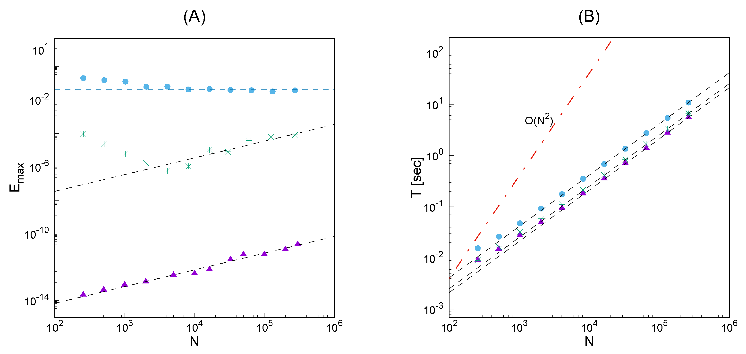

Table 1.
Absolute error of the computed Legendre coefficients for four different functions with different degree of smoothness (see text). The reference “exact” values of have been computed with 30 significant figures by standard quadrature with Mathematica [29].
Table 1.
Absolute error of the computed Legendre coefficients for four different functions with different degree of smoothness (see text). The reference “exact” values of have been computed with 30 significant figures by standard quadrature with Mathematica [29].
| 0 | 8.15 | 7.51 | 1.11 | 3.33 |
| 1 | 2.98 | 1.44 | 3.33 | 5.55 |
| 2 | 3.12 | 1.86 | 3.88 | 1.97 |
| 3 | 5.43 | 9.20 | 3.39 | 2.87 |
| 4 | 3.41 | 1.07 | 4.72 | 3.36 |
| 5 | 2.53 | 1.30 | 5.47 | 1.58 |
| 6 | 9.28 | 1.14 | 4.50 | 1.96 |
| 7 | 1.09 | 9.75 | 4.22 | 2.54 |
| 8 | 1.99 | 4.29 | 3.18 | 2.63 |
| 9 | 1.27 | 6.10 | 3.94 | 2.90 |
| 10 | 1.87 | 5.74 | 1.65 | 2.93 |
| 11 | 7.50 | 4.45 | 1.54 | 9.71 |
| 12 | 1.16 | 1.79 | 1.94 | 2.04 |
| 13 | 2.20 | 3.32 | 3.60 | 1.67 |
| 14 | 1.56 | 8.43 | 7.36 | 2.37 |
| 15 | 2.75 | 9.81 | 4.18 | 2.06 |
Disclaimer/Publisher’s Note: The statements, opinions and data contained in all publications are solely those of the individual author(s) and contributor(s) and not of MDPI and/or the editor(s). MDPI and/or the editor(s) disclaim responsibility for any injury to people or property resulting from any ideas, methods, instructions or products referred to in the content. |
© 2020 by the author. Licensee MDPI, Basel, Switzerland. This article is an open access article distributed under the terms and conditions of the Creative Commons Attribution (CC BY) license (https://creativecommons.org/licenses/by/4.0/).
Copyright: This open access article is published under a Creative Commons CC BY 4.0 license, which permit the free download, distribution, and reuse, provided that the author and preprint are cited in any reuse.


