Preprint

Article

Development of Monthly Scale Precipitation Forecasting Model for Indian Subcontinent Using Wavelet Based Deep Learning Approach

Altmetrics

Downloads

120

Views

Comments

A peer-reviewed article of this preprint also exists.

Pavan Kumar Yeditha

,Anusha Ganapathiraju^†,Siva Shyam Sai Nandikanti^†,

Maheswaran Rathinasamy^*

Pavan Kumar Yeditha

,Anusha Ganapathiraju^†,Siva Shyam Sai Nandikanti^†,

Maheswaran Rathinasamy^*

^† Equal Contribution

This version is not peer-reviewed

Submitted:

18 May 2023

Posted:

19 May 2023

You are already at the latest version

Alerts

Abstract

An accurate and timely precipitation forecast is essential for water resources management in hydropower, irrigation, and reservoir control. The conventional methods are limited by their inability to capture the high precipitation variability in time and space. In the present work, a wavelet-based deep learning approach is adopted to forecast precipitation using the lagged monthly rainfall, local climate variables, and global teleconnections such as IOD, PDO, NAO, and Nino 3.4 as predictors. The method was tested and validated over the Krishna River Basin in India. Overall, the forecasting accuracy was higher using the wavelet-based hybrid models than the single-scale models. The proposed multi-scale model was then applied to the different climatic regions of the country, and it was shown that the model could forecast the rainfall at reasonable accuracy for different climate zones of the country.

Keywords:

Subject: Engineering - Civil Engineering

1. Introduction

Precipitation is the most crucial atmospheric parameter influencing the water cycle [1]. Extreme floods or severe droughts are caused either due to excessive or deficient precipitation that may further seed socioeconomic losses. Effective precipitation forecasting is an urgent need to plan water management activities in a country like India, which is majorly dependent on precipitation for agricultural activities, as more than 65% of the cultural land in the country is rain-fed.

Forecasting monthly and seasonal precipitation is paramount to providing the information required for agricultural planning and water management [2,3] for regions that depend on rainfall as the primary source for agricultural activities. Hence, reliable forecasts are required to help the farming community decide the type of crop based on the forecasted precipitation quantities. Effective precipitation forecasts several months in advance can help plan disaster early warning and preparations [4,5]. Therefore, one of the most important scientific issues in hydrology is precipitation forecasting, and numerous researchers carried out several works for forecasting monthly and seasonal forecasting using numerous approaches.

Several methods were developed in the past few decades for forecasting precipitation, and these methods are typically divided into numeric and empirical models [2,5,6,7]. Methods that use laws of physics for climate forecasting are called numeric models. Also, these models include the movement of wind, clouds, and moisture, which statistical models cannot perceive, making these models more convincing than statistical data-driven models. These models generally develop the relationship between land, ocean, and atmospheric variables based on the data obtained from GCMs based on physical equations [8,9]. Researchers like [10,11] conducted several climatic studies using this modeling approach. Empirical methods include hydro-meteorological predictand and predictor variables through mathematical models based on historical data. The developed relationship is then used for data sets other than sample data to make forecasts. But due to uncertainty in model structure, parameters, initial conditions, and complexity, precipitation forecasting using numeric models cannot produce good precipitation forecasts [13]. Numerous works [7,8,13,14] show that empirical models have better accuracy in precipitation forecast when compared to physical based models due to higher uncertainties, whereas statistical models are based on historical data and mathematical approach. Empirical models are mainly used for seasonal forecasts in agricultural planning. Empirical models which are used for the development of forecasts are Multiple Linear Regression (MLR) [13], Artificial Neural Networks (ANN) [15].

It is believed that global teleconnection patterns, also known as large-scale climatic indices like Indian Ocean Dipole (IOD), North Atlantic Oscillation (NAO), NINO 3.4, and Pacific Decadal Oscillation (PDO), are influencing the rainfall variability across the globe and has been used as predictors of global precipitation [16].

Most of the above-reported studies have considered the global climatic predictor variables with historical data to develop precipitation forecasting models [17] but could not produce good reliable forecasts due to the non-stationary relationship between predictor variables and precipitation. To address this issue, wavelet analysis (WT) was used, and researchers did several works to develop models which can produce more reliable forecasts than singular models. Some works include developing a self-organizing map coupled with WT filters for forecasting monthly precipitation in Chile by [2,16] developing a wavelet-based non-linear model for forecasting monthly precipitation with climate data sets as predictors for the Cauvery basin in India. The results show that wavelet-coupled models produce good and reliable forecasts compared to singular models.

In [15] developed wavelet-based ANN models for forecasting monthly precipitation models for Australia and showed improved forecasting accuracy using multi-scale models.

In recent years, Extreme learning machines have been used for forecasting drought index, groundwater levels, and streamflow forecasting by numerous researchers who found that the results of this model showed reliable forecasts when compared to other forecasting models [18,19,20]. But the application of ELM to precipitation forecast was not carried out on a large scale by many works based on previous literature. Therefore, in this study, the applicability of a new and more effective precipitation forecast model for seasonal and monthly levels is proposed using Extreme Learning Machines (ELM) and Wavelet-based Extreme Wavelet Machines (WT-ELM) using large-scale climate indices and also other climatic predictor variables for Indian region. Recent literature suggests little work incorporating deep learning methods for precipitation forecasting in the Indian region. The main objectives of the work area

1. Development of singular ELM and WT-ELM for precipitation forecasting at a monthly and seasonal level using climate indices and local climatic predictor variables.

2. Comparison of the proposed approach with other methods, such as Multiple Linear Regression models, Artificial Neural Networks, and the Wavelet Neural Network approach at the country and basin scale.

2. Study Area and Data Used

To test the proposed approach in this work, a monthly precipitation forecast is carried out for the Krishna River basin, India, and the methodology is extended to the entire Indian sub-continent. India is a country that is majorly dependent on rainfall carrying out agricultural activities in the country India receives an average annual rainfall of 650 mm of rainfall every year, with more than 70% of the rainfall being received during the southwest monsoon (June to September) every year but the quantity of rainfall received is unreliable. In the case of the Northeast monsoon, the regions in India which did not receive rainfall during the SW monsoon, like the Tamil Nadu region, fed during the NE monsoon; around 50 to 60% of rainfall received by this region is during this monsoon. The rainfall received during the monsoons received is not uniformly spread along the country; thus, there is a need to determine the quantity received in each region to plan management activities. Climatic conditions also play a vital role in determining the quantity of rainfall received in a region. Indian climate is classified into six subtypes based on the Koppen climate classification: alpine tundra in the north, arid deserts in the west, and tropical rainforests in the southwest. The presence of microclimate regions makes the climate of India more diverse. The geographical variation of the Koppen climate for India is shown in Figure 1.

Krishna river basin is the 4^th largest river basin in India which receives around 400 to 4000mm of mean annual rainfall, out of which 90% of the rainfall is received during the Southwest monsoon and around 78% percentage of the area is agricultural land out of the total catchment area of 2,60,401 km². The basin is divided into three major climatic regions based on the Koppen climate classification, as shown in Figure 1, which constitute Tropical Monsoon, Tropical Savanna, and Semi-Arid climate. The precipitation variability in the basin can be understood from Figure 2b, which shows that the western region receives the highest rainfall.

Rainfall Data

Daily rainfall data is available at the spatial resolution of 0.25^° x 0.25^° gridded data and is obtained from Indian Metrological Department for each year from 1901 to 2018. This work uses the entire data to develop a model for forecasting precipitation at the country and basin levels. To develop models for monthly, the daily precipitation data is converted to monthly precipitation. The daily precipitation data set is downloaded from the website http://www.imdpune.gov.in/Clim_Pred_LRF_New/Grided_Data_Download.html.

Global Predictors Data

In this work, some of the global teleconnections that have been shown to influence precipitation have been considered. Apart from the global teleconnection patterns, regional climatic variables like temperature, pressure, and geopotential heights have been considered.

(i.): Indian Ocean Dipole (IOD), also called Indian Nino, is an irregular oscillation of sea surface temperature in the western Indian Ocean and affects rainfall variability in East Africa, India, Indonesia, and Southern Australia[22]. IOD is one of the major climate drivers for rainfall in India and is also referred to as the difference in sea surface temperature (SST) anomalies in the region in IOD West at 50 E to 70 E and also IOD East at 10 S to 10 N. Data is downloaded from https://www.esrl.noaa.gov/psd/gcos_wgsp/Timeseries/Data/dmi.long.data and is available at monthly scale from the period of 1870 to 2018.
(ii.): North Atlantic Oscillation (NAO) is a weather phenomenon that occurs in the North Atlantic Ocean, and its fluctuations are calculated based on the difference between subpolar low and subtropical high. Monthly data for these climatic indices can be obtained from the NOAA climate prediction Centre (CPC). The data is available for each month from 1948 to 2018.
(iii.): Nino 3.4 index: El Nino and La Nina events are most commonly defined by Nino 3.4 index. The anomalies of Nino 3.4 are thought to represent east-central Tropical Pacific SSTs. The data is available from 1870 to 2019 on a monthly scale.
(iv.): Pacific Decadal Oscillation (PDO) is often referred to as El Nino but acts at a larger scale, with a pattern mostly observed in North Pacific [23]. Extreme phases of the PDO index have been classified as warm or cool based on the ocean temperature anomalies in the tropical and northeast Pacific Ocean, and the length of the data available is from 1948 to 2018. The NAO, NINO 3.4, and PDO data are downloaded from https://www.esrl.noaa.gov/psd/data/climateindices/list/.

Apart from these climate indices, local predictor variables are used for forecasting precipitation. The details of Global climate and local predictor variables used in this study are shown in Table 1. The data from the local predictor variables were obtained from the NCEP-NCAR reanalysis dataset.

3. Methods

In this work, singular machine learning, deep learning models, and Hybrid models using wavelet decomposition were developed for monthly precipitation forecasting for the Krishna River basin as a case study. Later, based on the results from the case study, the best models were applied at the country level.

This section briefly describes wavelets, extreme learning machines, and hybrid modelling approaches. A further detailed description of the other traditional methods adopted is explained in sections A1- to A-2.

3.1. Wavelet Transform (WT)

Wavelet Transform is a mathematical tool that represents and analyzes a time series in both the time and frequency domains due to its multi-resolution and localization capabilities [24]. In recent decades the usage of wavelets in various domains of water resources and hydrology increased due to their capability to study non-stationarity in a time series [23,24,25]. Wavelets are broadly classified into two types: Continuous Wavelet transforms (CWT) and Discrete Wavelet transforms (DWT). Continuous wavelets transform works on all the scales to analyze a time series, whereas Discrete wavelet transform uses only dyadic scales. Based on several studies [26,27,28], Discrete wavelet transform can be obtained either by Mallet or by

\overset{´}{a}

trous wavelet transform and is also referred to as Maximum Overlap Discrete Wavelet Transform (MODWT). The main concept of MODWT is to fill the gaps using redundant information in the original series by passing it through a low pass filter to smoothen the data and retrieve details from the series [30].

Mathematically the smoother version of the original time series

x (t)

can be understood using Equation (1)

x (t) = P_{o} (t) P_{k} (t) = \sum_{m = - \infty}^{\infty} j (m) P_{k} (t + 2^{k - 1} m)

(1)

where

m

is the lowpass with compact support by a B₃ spline and defined by the values (1/16, 1/4, 3/8, 1/4, 1/16) & for Haar wavelet

m

is defined at (1/2, 1/2) and

k_{}

denotes the level of decomposition and takes the value from 1, 2, 3 ….

k

[30]

The detail component of the smoother version of

x (t)

for

k^{t h}

level can be mathematically expressed as in Equation (2)

d_{k} (t) = P_{k - 1} (t) - P_{k} (t)

(2)

where

P_{k}

is the approximation or residual component from wavelet decomposition and {

d_{1}, d_{2} \dots . d_{k}

} represents the additive wavelet decomposition of the data up to resolution level

k

. Wavelet decomposition of the time series is carried out using the WMTSA toolbox in MATLAB.

3.2. Extreme Learning Machines (ELM)

Understanding complicated relationships between multiple parameter-dependent variables like precipitation is difficult due to its strong influence on different climatological parameters. Several studies have shown the efficacy of ELMs in capturing non-linear relationships using the single hidden layer feed-forward networks (SLFNs) to train the datasets. Hung first proposed this method in 2004 due to its fast learning and high generalization and did not create dependency among the different layers as in ANNs. The performance of ELMs, such as lower error components and generalization in performance, was checked by [31] which justifies the principle of this method. In this method, the only free component is weighted between the hidden and output layers, and the hidden nodes need not be similar to neurons [32]. The hidden nodes can be expressed as [31,33]

\sum_{i = 1}^{k} B_{i} h_{i} (α_{i} x_{i} + β_{i}) = z_{i}

(3)

where the output weight vector between

k

number of nodes to the output nodes is given by

B

, the hidden layer activation function is given by

G (α, β, x)

, and Z represents the ELM model's output.

α, β

are the biases in the ELM algorithm's randomized layers. For the present study, the number of neurons was selected as 1-20, and the sigmoidal function was chosen as activation function f(x) following previous studies by [34,35]

f (x) = \frac{1}{1 + \exp (- x)}

(4)

As explained by [31], the approximate set of N sample data sets can be obtained by using Equation (5)

\sum_{t = 1}^{N} ‖z_{t} - y_{t}‖

(5)

where

z_{t}

denote the ELM model output at data points

t = 1,2, 3, \dots N

and

y_{t}

are the response variables, i.e., the observed precipitation values used to validate precipitation forecasts.

Finally, the forecasted values of the data sets

\hat{y}

can be obtained by testing the input vector (

x_{t e s t}

) [36] using Equation (6)

\hat{y} = \sum_{i = 1}^{k} {\hat{B}}_{i} h_{i} (α_{i} . x_{t e s t} + β_{i})

(6)

where

{\hat{B}}_{}

represents the estimated output weights from the N data samples used in modelling processes [31]. For a more detailed understanding of ELM readers, refer to [32]. A typical ELM is represented in Figure 3.

3.3. Wavelet Hybrid Models

In Wavelet Hybrid models, the decomposed components of the original series and climate predictor variable are used to improve the quality of precipitation forecast. As mentioned in Section 3.1, decomposition is carried out using Maximal Overlap Discrete Wavelet Transform (MODWT). The capability of Wavelet models to identify hidden relationships among predictand and predictors by decomposition of the variables is the main advantage of using Wavelet decomposition.

In this work, Feed Forward Back Propagation Neural network model (FFPBP-NN) based on previous literature and ELM models are coupled with wavelets to develop wavelet Hybrid Models. These models are denoted as WT-FFBP-NN and WT-ELM. A detailed description of FFBP-NN and Multiple Linear Regression models is provided in Appendix A.1 and A.2.

4. Methodology

STEP: Identification of Significant Variables

Based on the literature, precipitation is assumed to respond to large-scale climate signals and local predictors with time lags. Auto Correlation Function (ACF) and Cross-Correlation Function (CCF) are the lags at which the predictor variables influence the precipitation. Based on CCF, the lag correlation of various predictor variables is determined and used to develop forecasting models.

STEP:1 Selection of predictor variables

After the first step, the climate predictor variables are chosen based on the values of correlation and Cross-Correlation Function (CCF) to determine the predictor monthly and seasonal subseries of lag components with precipitation. Some of the sample correlation plots are shown in Figure 4. The correlation of climatic indices at different lag values is shown in Figure 4 at monthly scales to determine the lag component at which the indices are closely related to precipitation time series.

It can be seen that each index has varying relationships with precipitation. Based on these values, the component of indices to be used in the analysis are selected. These climatic indices and predictors are selected based on previous works[2], [34,35] Also, along with the lagged values, zero lag coefficients are also used as the presence of long-term and short-term memory[39].

STEP 2 Standardization

After selecting predictor variables, the data sets are standardized to reduce the effect of the difference in magnitude between different variables. In this work, the standardization of variables is carried out using Equation (7)

x_{s t d} = \frac{x - x_{m i n}}{x_{m a x} - x_{m i n}}

(7)

where

x

represents the predictor variables,

x_{s t d}

= standardized value of predictor variables,

x_{m i n}

and

x_{m a x}

represent the minimum value and maximum value of predictor variable

x .

Step 3: Model development

(a): Single scale models (MLR, FFBP-NN, ELM)

After selecting probable predictors based on correlation and CCF of variables with monthly precipitation time series based on lag components, the entire data set is divided into 70:30 ratios. Training of the models is carried out using 70 % of the data set, and validation of the models is carried out using the remaining 30% of the data, and the performance of these models is evaluated using the performance measures mentioned in Section 3(c).

(b): Wavelet Hybrid models (WT-FFBP-NN and WT-ELM)

MODWT is applied to the predictor variables after selecting suitable potential predictors to decompose the data sets at various scales. As mentioned by [30], selecting suitable mother wavelets and level of decomposition help capture required features that provide information for good results. An optimum decomposition level and mother wavelet choice are selected based on the works [40] and [28,35] The lagged decomposed predictor variables are given as input for both WT-FFBP-NN and WT-ELM models.

(c): Performance Measures

This study verifies the accuracy and confidence limit of the model's forecast using statistical metrics. The measures used in this study are Root Mean Square Error (RMSE), Correlation (R²), Nash Sutcliffe Efficiency (NSE), and Most Absolute Error (MAE).

If the values of RMSE are high, the error component in the forecast to the original system is large. Whereas if the values of NSE and Correlation are nearer to 1, the obtained results are nearer to the original system. If the values are nearer to 0, the model output is not a correct representation of the original system. RMSE and MAE represent the error component in the out of the models.

i.: Root Mean Square Error (RMSE)

R M S E = \sqrt{\frac{1}{n} \sum_{i = 1}^{n} {(X_{i}^{o b s} - X_{i}^{s i m})}^{2}} X 100 %

(8)

ii.: Correlation (R²)

R^{2} = {(\frac{\sum_{i = 1}^{n} (x_{i}^{o b s} - x_{m e a n}^{o b s}) (x_{i}^{s i m} - x_{m e a n}^{s i m})}{\sqrt{\sum_{i = 1}^{n} {(x_{i}^{o b s} - x_{m e a n}^{o b s})}^{2} {(x_{i}^{s i m} - x_{m e a n}^{s i m})}^{2}}})}^{2}

(9)

iii.: Nash Sutcliffe Efficiency (NSE)

N S E = 1 - \frac{\sum_{i = 1}^{n} {(X_{i}^{o b s} - X_{i}^{s i m})}^{2}}{\sum_{i = 1}^{n} {(X_{i}^{o b s} - X_{i}^{s i m m e a n})}^{2}}

(10)

iv.: Most Absolute Error (MAE)

M A E = \frac{\sum_{i = 1}^{n} | (X_{i}^{o b s} - X_{i}^{s i m}) |}{n}

(11)

where

X_{i}^{o b s}

represent the ith observed data,

X_{i}^{s i m}

represent the simulated data from the models,

X_{i}^{m e a n}

is the mean of the data set, and n is the number of observations.

5. Results and Discussions

5.1. Forecasting using Single Scale Models

Training and validation of all the models, including hybrid models such as Wavelet Hybrid models (WT-FFBP-NN and WT-ELM), were done using performance measures (Section 3(c) until satisfactory results in terms of NSE and RMSE for precipitation forecasting were obtained. To test the efficacy of the models, five locations (one from each climate classification) in the Krishna River basin were selected for the development of models and analysis of precipitation in the basin.

For the Krishna River basin

Results of the models using only global climate indices as predictors

The results obtained from all the models using only the global climate indices and lagged precipitation data are shown in Table 2. The results show that MLR models obtained correlation values ranging from 0.30-0.37 and NSE values from 0.11 to 0.16. For FFBP-NN models, the forecast results showed correlation values ranging from 0.66-0.73 and NSE ranging from 0.44 to 0.52. The results from the ELM model had a correlation ranging from 0.34-0.56 and NSE in the range of 0.34 -0.51 for the five stations considered. WT-FFBP-NN model results yielded NSE values of 0.38-0.40 with a correlation of 0.56-0.64.

WT-ELM models showed an improved performance in terms of NSE and CC compared to the other models, as shown in Table 2.

(a): Results of the models using only local climate variables as predictors

Table 3 shows the results of the models for the Krishna River basin at all the selected locations at a monthly scale with only local predictors variables as inputs. The results show that the MLR model has correlation values ranging from 0.57 to 0.68 for the five locations, and the NSE values ranged between 0.32 -0.40.

Comparative results were obtained using FFBP-NN and ELM models where the NSE values ranged between 0.44-0.52 for the former and 0.43-0.50 for the latter, respectively. However, in the case of the results from WT-FFBP-NN and WT-ELM show higher values, with NSE values ranging between 0.50-0.56 and 0.51-0.57, respectively.

c. Results of models with both global climate variables and local predictor variables

In this case, local and global climate variables were considered along with the lagged precipitation for forecasting.

The results shown in Table 4 show a considerable increase in the model accuracy in terms of NSE, RMSE, and MAE. Further, it is also observed that the wavelet-based hybrid models, WT-FFBP-NN and WT-ELM, provided better forecasts than the other models. The best model was the WT-ELM, with the NSE ranging from 0.62-0.85 and the correlation coefficient in the range of 0.77-0.92.

It was also observed that the models using only global climate indices as inputs obtained the highest NSE value of 0.52, and the models using local predictor variables obtained the highest value of 0.67. Whereas for the models with global climate and local predictor variables as inputs, the NSE values were increased to an average of 28% compared to those with only local predictor variables. Therefore, from the results for all the stations, the highest correlation was obtained for WT ELM for station 1 with a value of 0.92, followed by WT FFBP-NN with the highest NSE value of 0.85. Similarly, the best results for all the other stations were obtained for WT ELM models. Overall, the values NSE and correlation show that WT ELM outperformed WT FFBP-NN models and other singular models in precipitation forecasting for the Krishna River basin.

Overall, it was observed that including both the global and local predictors improved precipitation accuracy. It was also observed that the results based on the Wavelet-based models were more accurate compared to the other singular models considered in the study. When these models were coupled with wavelets, the model could capture the nonlinearity, which helped the WT ELM models to capture all the necessary details and produce reliable precipitation forecasts.

Further comparing the model results obtained from WT-ELM and WT-FFBP-NN models, the WT-ELM based showed superior performance. It is clear that by coupling machine learning models with Wavelets, the forecasting capabilities of the models have increased with the results which registered low values when modeled with basic models were found to be improved while usage of WT-based hybrid models for forecasting.

Model Application for the Different Regions in India

Based on the results obtained for the Krishna River basin, the best model was the WT- ELM model. So, to test the model results for the entire country and generalize the model performance, WT-ELM models were developed for the chosen 4 locations for each region categorized by IMD based on precipitation. The results for the selected locations are shown in Table 5.

Central India:

The results from the models show that the correlation values found to be 0.90,0.87,0.92 and 0.87, with the NSE values being 0.81,0.72,0.85,0.75 and the values of MAE showing that the error component in the forecast is relatively low as the value is nearer to zero. Also, the value of RMSE is less than 0.08 for all the stations.

North India:

The results from the WT-ELM models show that the correlation values are 0.84,0.88,0.82, and 0.78 with NSE values of 0.70,0.77,0.68, and 0.54, along with low MAE and RMSE values. These low RMSE and RMSE indicate that the error component in the forecasting model is less.

Peninsular India:

The correlation values from the results show that values are 0.84,0.79,0.92, and 0.87, respectively, for the four selected stations with NSE values of 0.66,0.61,0.85, and 0.76. The values of MAE were also found to be low, similar to the results of the remaining regions.

Northwest:

The results indicate that the correlation values in these regions are 0.91,0.88,0.76, and 0.83, with NSE values of 0.84,0.74,.50, and 0.67.

Based on the results in Table 3, Table 4 and Table 5, the model that produced good results for all the different input combinations is the WT-ELM model with the highest correlation, highest NSE, and the lowest error component than linear MLR model, machine learning models like FFBP-NN, ELM, and WT-FFBP-NN.

Figure 5. Spatial map of NSE for various models for India using (a) FFBP-NN, (b) ELM, (c) WT FFBP-NN, and (d) WT-ELM models.

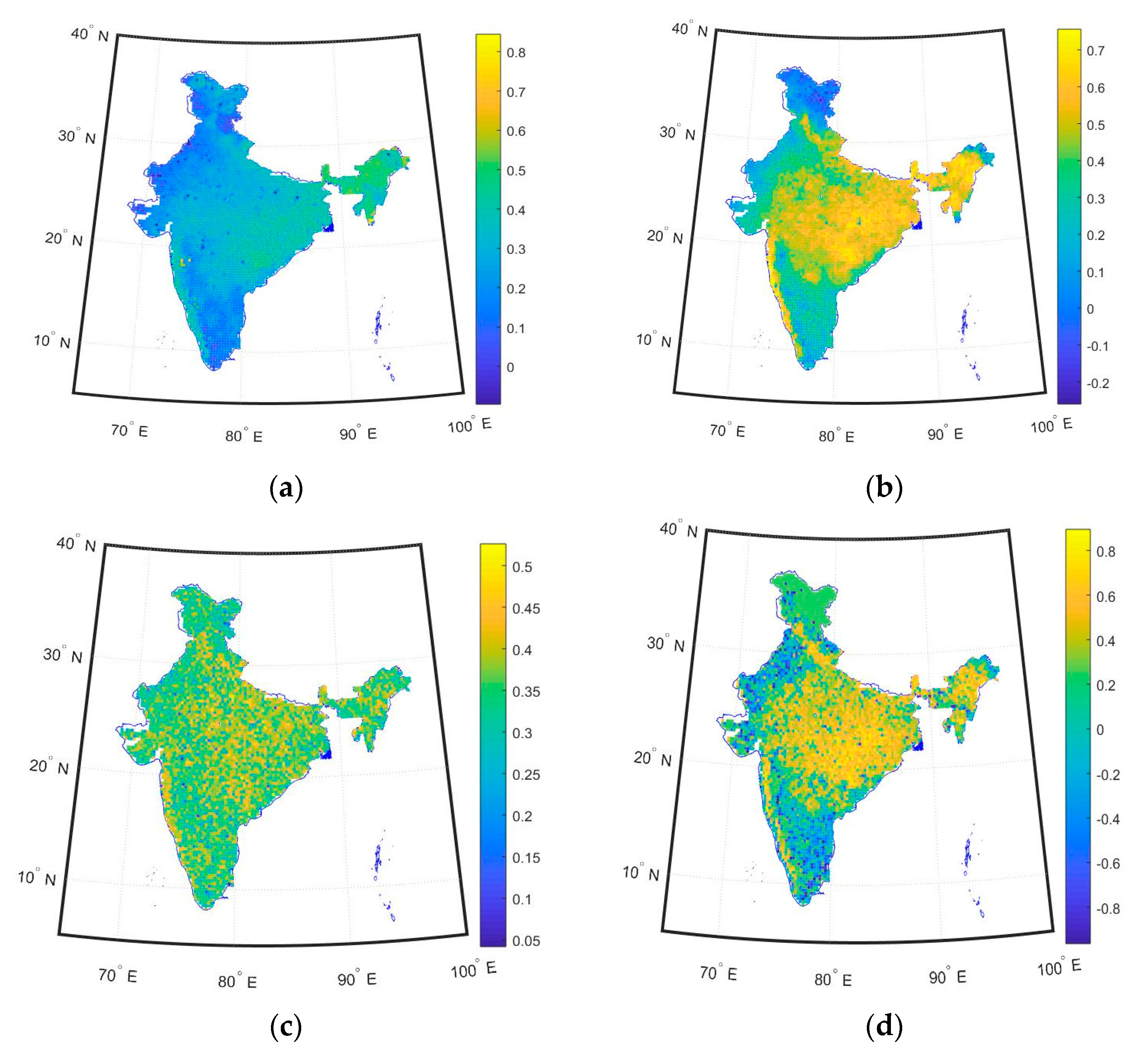
Discussion

In this study, wavelet-based hybrid models were tested for their ability to forecast monthly precipitation, and their performances were compared with those of some key traditional and other contemporary methods, including MLR, FFBP-NN, and ELM models. Among the different forecasting methods applied in this study, machine learning methods generally outperform the basic MLR models. Among the single-scale machine learning models, the ELM model outperformed the FFBP-NN model. The better performance of the ELM model may be due to its ability to capture the long- and short-term memory relationship between the climatic variables and precipitation.

Overall, our results manifest that the wavelet-based hybrid models (WT-FFBP-NN and WT-ELM) are accurate compared to the traditional and other machine-learning methods considered in this study. This observation is in congruence with the broader understanding of the performance of the wavelet-based hybrid models, where in wavelets enhance the models' capability to unravel the multi-scale relationship among the variables. For example, in a recent study,[41] showed that wavelet-based decomposition helps identify the correlation between different variables, improving the model skill score. Similarly, in another study by [29], the authors showed that the Wavelet-based models are accurate for streamflow forecasting. Another study,[42] showed that the wavelet based Volterra model performed superior to the simple non-linear models for rainfall forecasting.

To understand the possible reasons for improving the performance of the Wavelet-based models, the correlations between the precipitation and climatic variables with and without wavelet decomposition. Table 6 shows the values of the same for Grid 2.

The correlation between precipitation and geopotential height (p850) is –0.06 without applying wavelet decomposition; conversely, the correlation is on the order of -0.47 to -0.16 between decompositions of p850 (D4 to D9), and precipitation varies from –0.17 to –0.39. A similar kind of correlation can also be observed for several other variables (e.g., uas, p500, mlp). Overall, it is observed that there is a significant improvement in the correlation, or in other words, wavelets can unravel the hidden relationships and improve the performance of the forecasting models.

It is pertinent to understand that the NCEP reanalysis data has been used; however, the methodology can be extended to the weather forecasting model results and used to extend the forecast lead time.

6. Conclusions

In this study, singular machine learning and Wavelet hybrid models were developed and applied to predict monthly precipitation for the Krishna River basin using local and global climate data as predictor variables. Based on the results obtained from evaluation measures, the model with the best prediction capability was found, and their ability to capture extreme events was identified. The performance measures showed that WT ELM models captured the events with higher precision than WT FBP-NN models with lower RMSE and higher NSE values. The outcome of this study indicates the capability of WT ELM models in forecasting works, and its applicability can be understood from the results from the case study for the Krishna River basin. Further evaluation of this model can be understood by adopting a similar methodology to analyze works for various regions with different climatic and metrological factors.

Author Contributions

Conceptualization, RM. and Y.P.; methodology, RM and YP, GA.; software, GA and YP; validation RM, YP and GA.; formal analysis, SSSN.; investigation, SSSN and GA; resources, SSSN, GA and YP.; data curation, YP , GS and SSSN.; writing—original draft preparation, YP and GA, SSSN; writing—review and editing, RM; visualization, YP and SSSN.; supervision,RM.; project administration, RM.; funding acquisition, RM. All authors have read and agreed to the published version of the manuscript.

Funding

This research was funded by the name of IIT H, grant number SEED GRANT/SG114.

Data Availability Statement

The data used in this study can be made available from the sources mentioned in the manuscript.

Acknowledgments

RM gratefully acknowledges the SEED Grant (SG-114) funding from IIT Hyderabad, India.

Conflicts of Interest

The authors declare no conflict of interest.

Appendix A

A-1 Multiple learning regression (MLR)

Multiple linear regression is a form of linear regression analysis which develops the relationship between multiple predictor variable (

x_{1} {, x}_{2,} x_{3,} \dots . x_{n}

) with respect to predictand variable (y) and this relationship can be understood using Eq (A-1)

y = a_{1} + a_{2} x_{1} + a_{2} \dots . a_{n} x_{n}

where

a_{1}, a_{2}, a_{3} \dots . a_{n}

are calculated using the simple least squares method. A detailed explanation of the MLR model can be understood by referring to [43].

A-2 ARTIFICIAL NEURAL NETWORKS (ANN)

Artificial Neural Networks are defined signal processing using neurons which save required experimental data to use for further processes. ANN has been developed to resemble the biological nervous system and they learn, store and process data sets based on examples. Understanding complex relationships between inputs and targets, which is not possible using linear algorithms can be performed easily and with high accuracy using ANNs [44]. ANNs have been used for a few decades in various fields for the analysis of different kinds of problems in hydrology and climatology. The application of this method can be further understood by seeing works like [30,45,46,47,48,49]. The ability of ANNs to learn and simulate the results based on the provided inputs show its capability to solve complex problems which linear models cannot perform [50]. Further the structure and capabilities of ANNs can be understood in detail by referring to [42,51,52]. While training a network, the number of neurons is varied numerous times by using the trial-and-error method until the satisfaction of minimum criteria error [53]. Numerous training functions were available for training Neural networks to understand and capture input-output relationships. Some of the functions are Feed-Forward Back Propagation Neural Network (FFBP-NN), Non-linear Auto Regressive with exogenous inputs Neural Network (NARX-NN), and Generalized Regression Neural Network (GRNN). In this work, for the application of models, FFBP-NN models were used for forecasting precipitation due to their higher applicability than other models. For a detailed understanding of this model, readers can refer to the works of [54,55], among others.

The FFBP-NN is a multiple-layer network which consists of neurons that are stacked in layers and connected with each other. Inputs and outputs of the networks are the first and last layers of the networks with hidden layers being the remaining layers that carry information in the form of weights. In this study, FFBP-NN is trained, which is most widely used, especially in hydrologic applications. In this model, input data in the layers include input data is given by

x_{1}, x_{2}, x_{3} \dots . x_{n}

and the results from the output layer are given as

y_{1}, y_{2}, y_{3} \dots . y_{n}

. the input neurons are connected with hidden layers by the weights, which connect the t^th neuron and the k^th neuron, represented by

w_{t k}

. Whereas

w_{j t}

represents the connection between hidden layers and wtthe outputs layer. Being non-linear functions, ANNs capture the relationship between the input and output layer and the correlation for output can be understood [56] by Equation (A-2)

y_{j} = f_{o} (\sum_{t = 1}^{s} w_{j t} . f_{h} (\sum_{t = 1}^{s^{'}} w_{t k} x_{k} + b_{t}) + b_{j})

where

f_{o}

and

f_{h}

denote the activation function in the output layer and the activation function of nodes in the hidden layer.

b_{t}

and

b_{j}

are bias of tth neuron and jth neuron.

s a n d s^{'}

represent the nodes in the input and hidden layer respectively.

The training algorithm used in the development of FFBP-NN model is Levenberg-Marquardt (LM) which is assumed to be one of the fastest and accurate due to the recurrence to incorporate experience in training processes [36].

References

K. E. Trenberth, L. Smith, T. Qian, A. Dai, and J. Fasullo, “Estimates of the global water budget and its annual cycle using observational and model Data,” Journal of Hydrometeorology, vol. 8, no. 4. pp. 758–769, Aug. 2007. [CrossRef]
R. Abdi and T. Endreny, “A river temperature model to assist managers in identifying thermal pollution causes and solutions,” Water (Switzerland), vol. 11, no. 5, May 2019. [CrossRef]
R. Maheswaran and R. Khosa, “A Wavelet-Based Second Order Nonlinear Model for Forecasting Monthly Rainfall,” Water Resources Management, vol. 28, no. 15, pp. 5411–5431, Dec. 2014. [CrossRef]
L. Xu, N. Chen, X. Zhang, and Z. Chen, “A data-driven multi-model ensemble for deterministic and probabilistic precipitation forecasting at seasonal scale,” Clim Dyn, vol. 54, no. 7–8, pp. 3355–3374, Apr. 2020. [CrossRef]
A. G. Yilmaz and N. Muttil, “Runoff Estimation by Machine Learning Methods and Application to the Euphrates Basin in Turkey,” J Hydrol Eng, vol. 19, no. 5, pp. 1015–1025, May 2014. [CrossRef]
G. L. Feng et al., “Improved prediction model for flood-season rainfall based on a nonlinear dynamics-statistic combined method,” Chaos, Solitons and Fractals, vol. 140. Elsevier Ltd, Nov. 01, 2020. [CrossRef]
L. Cuo, T. C. Pagano, and Q. J. Wang, “A review of quantitative precipitation forecasts and their use in short- to medium-range streamflow forecasting,” Journal of Hydrometeorology, vol. 12, no. 5. pp. 713–728, Oct. 2011. [CrossRef]
Z. Hao, V. P. Singh, and Y. Xia, “Seasonal Drought Prediction: Advances, Challenges, and Future Prospects,” Reviews of Geophysics, vol. 56, no. 1, pp. 108–141, Mar. 2018. [CrossRef]
H. S. Bauer et al., “Quantitative precipitation estimation based on highresolution numerical weather prediction and data assimilation with WRF - a performance test,” Tellus, Series A: Dynamic Meteorology and Oceanography, vol. 67, no. 1, 2015. [CrossRef]
D. J. Stensrud et al., “Convective-scale warn-on-forecast system: A vision for 2020,” Bull Am Meteorol Soc, vol. 90, no. 10, pp. 1487–1499, 2009. [CrossRef]
S. K. Saha et al., “Improved simulation of Indian summer monsoon in latest NCEP climate forecast system free run,” International Journal of Climatology, vol. 34, no. 5, pp. 1628–1641, 2014. [CrossRef]
F. Molteni, R. Buizza, T. N. Palmer, and T. Petroliagis, “The ECMWF Ensemble Prediction System: Methodology and validation,” 1996.
B. Choubin, S. Khalighi-Sigaroodi, A. Malekian, and Ö. Kişi, “Multiple linear regression, multi-layer perceptron network and adaptive neuro-fuzzy inference system for forecasting precipitation based on large-scale climate signals,” Hydrological Sciences Journal, vol. 61, no. 6, pp. 1001–1009, Apr. 2016. [CrossRef]
L. Xu, N. Chen, X. Zhang, and Z. Chen, “An evaluation of statistical, NMME and hybrid models for drought prediction in China,” J Hydrol (Amst), vol. 566, pp. 235–249, Nov. 2018. [CrossRef]
M. Ghamariadyan and M. A. Imteaz, “A wavelet artificial neural network method for medium-term rainfall prediction in Queensland (Australia) and the comparisons with conventional methods,” International Journal of Climatology, vol. 41, no. S1, pp. E1396–E1416, Jan. 2021. [CrossRef]
R. K. Chowdhury and S. Beecham, “Australian rainfall trends and their relation to the southern oscillation index,” Hydrol Process, vol. 24, no. 4, pp. 504–514, Feb. 2010. [CrossRef]
J. Abbot and J. Marohasy, “Application of artificial neural networks to rainfall forecasting in Queensland, Australia,” Adv Atmos Sci, vol. 29, no. 4, pp. 717–730, Jul. 2012. [CrossRef]
D. Rivera, M. Lillo, C. B. Uvo, M. Billib, and J. L. Arumí, “Forecasting monthly precipitation in Central Chile: A self-organizing map approach using filtered sea surface temperature,” Theor Appl Climatol, vol. 107, no. 1–2, pp. 1–13, 2012. [CrossRef]
R. Barzegar, A. Asghari Moghaddam, J. Adamowski, and B. Ozga-Zielinski, “Multi-step water quality forecasting using a boosting ensemble multi-wavelet extreme learning machine model,” Stochastic Environmental Research and Risk Assessment, vol. 32, no. 3, pp. 799–813, Mar. 2018. [CrossRef]
M. Alizamir, O. Kisi, and M. Zounemat-Kermani, “Modelling long-term groundwater fluctuations by extreme learning machine using hydro-climatic data,” Hydrological Sciences Journal, vol. 63, no. 1, pp. 63–73, Jan. 2018. [CrossRef]
B. J. Li and C. T. Cheng, “Monthly discharge forecasting using wavelet neural networks with extreme learning machine,” Sci China Technol Sci, vol. 57, no. 12, pp. 2441–2452, Dec. 2014. [CrossRef]
C. C. Ummenhofer, A. Sen Gupta, M. H. England, and C. J. C. Reason, “Contributions of Indian Ocean sea surface temperatures to enhanced East African rainfall,” J Clim, vol. 22, no. 4, pp. 993–1013, Feb. 2009. [CrossRef]
M. Rathinasamy, A. Agarwal, B. Sivakumar, N. Marwan, and J. Kurths, “Wavelet analysis of precipitation extremes over India and teleconnections to climate indices,” Stochastic Environmental Research and Risk Assessment, vol. 33, no. 11–12, pp. 2053–2069, Dec. 2019. [CrossRef]
I. Daubechies, “The Wavelet Transform, Time-Frequency Localization and Signal Analysis,” IEEE Trans Inf Theory, vol. 36, no. 5, pp. 961–1005, 1990. [CrossRef]
M. Küçük, E. Tigli, and N. Ağiralioğlu, “Wavelet Transform Analysis For Nonstationary Rainfall-Runoff-Temperature Processes,” 2004. [Online]. Available: http://www.r-project.org.
J. Park and M. E. Mann, “Paper No. 1 • Page 1 Copyright,” 2000. [Online]. Available: http://EarthInteractions.org.
A. Grossmann and J. Morlet, “DECOMPOSITION OF HARDY FUNCTIONS INTO SQUARE INTEGRABLE WAVELETS OF CONSTANT SHAPE*,” 1984. [Online]. Available: https://epubs.siam.org/terms-privacy.
O. Renaud, J. L. Starck, and F. Murtagh, “Wavelet-based combined signal filtering and prediction,” IEEE Transactions on Systems, Man, and Cybernetics, Part B: Cybernetics, vol. 35, no. 6, pp. 1241–1251, Dec. 2005. [CrossRef]
J. Adamowski and K. Sun, “Development of a coupled wavelet transform and neural network method for flow forecasting of non-perennial rivers in semi-arid watersheds,” J Hydrol (Amst), vol. 390, no. 1–2, pp. 85–91, Aug. 2010. [CrossRef]
R. Maheswaran and R. Khosa, “Comparative study of different wavelets for hydrologic forecasting,” Comput Geosci, vol. 46, pp. 284–295, Sep. 2012. [CrossRef]
G. Bin Huang, Q. Y. Zhu, and C. K. Siew, “Extreme learning machine: Theory and applications,” Neurocomputing, vol. 70, no. 1–3, pp. 489–501, Dec. 2006. [CrossRef]
G. Bin Huang, “What are Extreme Learning Machines? Filling the Gap Between Frank Rosenblatt’s Dream and John von Neumann’s Puzzle,” Cognit Comput, vol. 7, no. 3, pp. 263–278, Jun. 2015. [CrossRef]
Z. M. Yaseen et al., “Stream-flow forecasting using extreme learning machines: A case study in a semi-arid region in Iraq,” J Hydrol (Amst), vol. 542, pp. 603–614, Nov. 2016. [CrossRef]
R. C. Deo and M. Şahin, “An extreme learning machine model for the simulation of monthly mean streamflow water level in eastern Queensland,” Environ Monit Assess, vol. 188, no. 2, pp. 1–24, Feb. 2016. [CrossRef]
R. C. Deo and M. Şahin, “Application of the Artificial Neural Network model for prediction of monthly Standardized Precipitation and Evapotranspiration Index using hydrometeorological parameters and climate indices in eastern Australia,” Atmos Res, vol. 161–162, pp. 65–81, Jul. 2015. [CrossRef]
P. Swapna et al., “The IITM earth system model : Transformation of a seasonal prediction model to a long-term climate model,” Bull Am Meteorol Soc, vol. 96, no. 8, pp. 1351–1368, Aug. 2015. [CrossRef]
H. L. Ren, B. Lu, J. Wan, B. Tian, and P. Zhang, “Identification Standard for ENSO Events and Its Application to Climate Monitoring and Prediction in China,” Journal of Meteorological Research, vol. 32, no. 6, pp. 923–936, Dec. 2018. [CrossRef]
V. Sehgal, A. Lakhanpal, R. Maheswaran, R. Khosa, and V. Sridhar, “Application of multi-scale wavelet entropy and multi-resolution Volterra models for climatic downscaling,” J Hydrol (Amst), vol. 556, pp. 1078–1095, Jan. 2018. [CrossRef]
S. Kannan and S. Ghosh, “Prediction of daily rainfall state in a river basin using statistical downscaling from GCM output,” Stochastic Environmental Research and Risk Assessment, vol. 25, no. 4, pp. 457–474, May 2011. [CrossRef]
A. Lakhanpal, V. Sehgal, R. Maheswaran, R. Khosa, and V. Sridhar, “A non-linear and non-stationary perspective for downscaling mean monthly temperature: a wavelet coupled second order Volterra model,” Stochastic Environmental Research and Risk Assessment, vol. 31, no. 9, pp. 2159–2181, Nov. 2017. [CrossRef]
Y. P. Kumar, R. Maheswaran, A. Agarwal, and B. Sivakumar, “Intercomparison of downscaling methods for daily precipitation with emphasis on wavelet-based hybrid models,” J Hydrol (Amst), vol. 599, Aug. 2021. [CrossRef]
R. Maheswaran and R. Khosa, “Wavelet Volterra Coupled Models for forecasting of nonlinear and non-stationary time series,” Neurocomputing, vol. 149, no. PB, pp. 1074–1084, Feb. 2015. [CrossRef]
D. J. Olive, “Prediction Intervals for Regression Models,” 2006.
M. J. Alizadeh, M. R. Kavianpour, O. Kisi, and V. Nourani, “A new approach for simulating and forecasting the rainfall-runoff process within the next two months,” J Hydrol (Amst), vol. 548, pp. 588–597, 2017. [CrossRef]
Ö. Kişi, “Neural Networks and Wavelet Conjunction Model for Intermittent Streamflow Forecasting,” J Hydrol Eng, vol. 14, no. 8, pp. 773–782, 2009. [CrossRef]
V. Nourani, M. Komasi, and A. Mano, “A multivariate ANN-wavelet approach for rainfall-runoff modeling,” Water Resources Management, vol. 23, no. 14, pp. 2877–2894, 2009. [CrossRef]
U. Okkan and O. Fistikoglu, “Evaluating climate change effects on runoff by statistical downscaling and hydrological model GR2M,” Theor Appl Climatol, vol. 117, no. 1, pp. 343–361, Sep. 2014. [CrossRef]
B. Ahmed and M. A. Al Noman, “Land cover classification for satellite images based on normalization technique and Artificial Neural Network,” in 1st International Conference on Computer and Information Engineering, ICCIE 2015, Institute of Electrical and Electronics Engineers Inc., Feb. 2016, pp. 138–141. [CrossRef]
M. T. Vu, T. Aribarg, S. Supratid, S. V. Raghavan, and S. Y. Liong, “Statistical downscaling rainfall using artificial neural network: significantly wetter Bangkok?,” Theor Appl Climatol, vol. 126, no. 3–4, pp. 453–467, Nov. 2016. [CrossRef]
D. E. Rumelhart, B. Widrow, and M. A. Lehr, “The Basic Ideas in Neural Networks,” Commun ACM, vol. 37, no. 3, pp. 87–92, 1994. [CrossRef]
R. J. Kuligowski and A. P. Barros, “Localized Precipitation Forecasts from a Numerical Weather Prediction Model Using Artificial Neural Networks,” 1998.
A. S. Tokar and M. Markus, “Precipitation-Runoff Modeling Using Artificial Neural Networks and Conceptual Models,” J Hydrol Eng, vol. 5, no. 2, pp. 156–161, Apr. 2000. [CrossRef]
R. Maheswaran and R. Khosa, “Wavelet Volterra Coupled Models for forecasting of nonlinear and non-stationary time series,” Neurocomputing, vol. 149, no. PB, pp. 1074–1084, 2015. [CrossRef]
S. Haykin, Neural Networks and Learning Machines, vol. 3. 2008. ISBN 978-0131471399.
S. Shanmuganathan, Studies in Computational Intelligence 628 Artificial Neural Network Modelling, vol. 628. 2016. [Online]. Available: http://www.springer.com/series/7092.
C. A. G. Santos, O. Kisi, R. M. da Silva, and M. Zounemat-Kermani, “Wavelet-based variability on streamflow at 40-year timescale in the Black Sea region of Turkey,” Arabian Journal of Geosciences, vol. 11, no. 8, Apr. 2018. [CrossRef]

Figure 1. Koppen Climate classification for India.

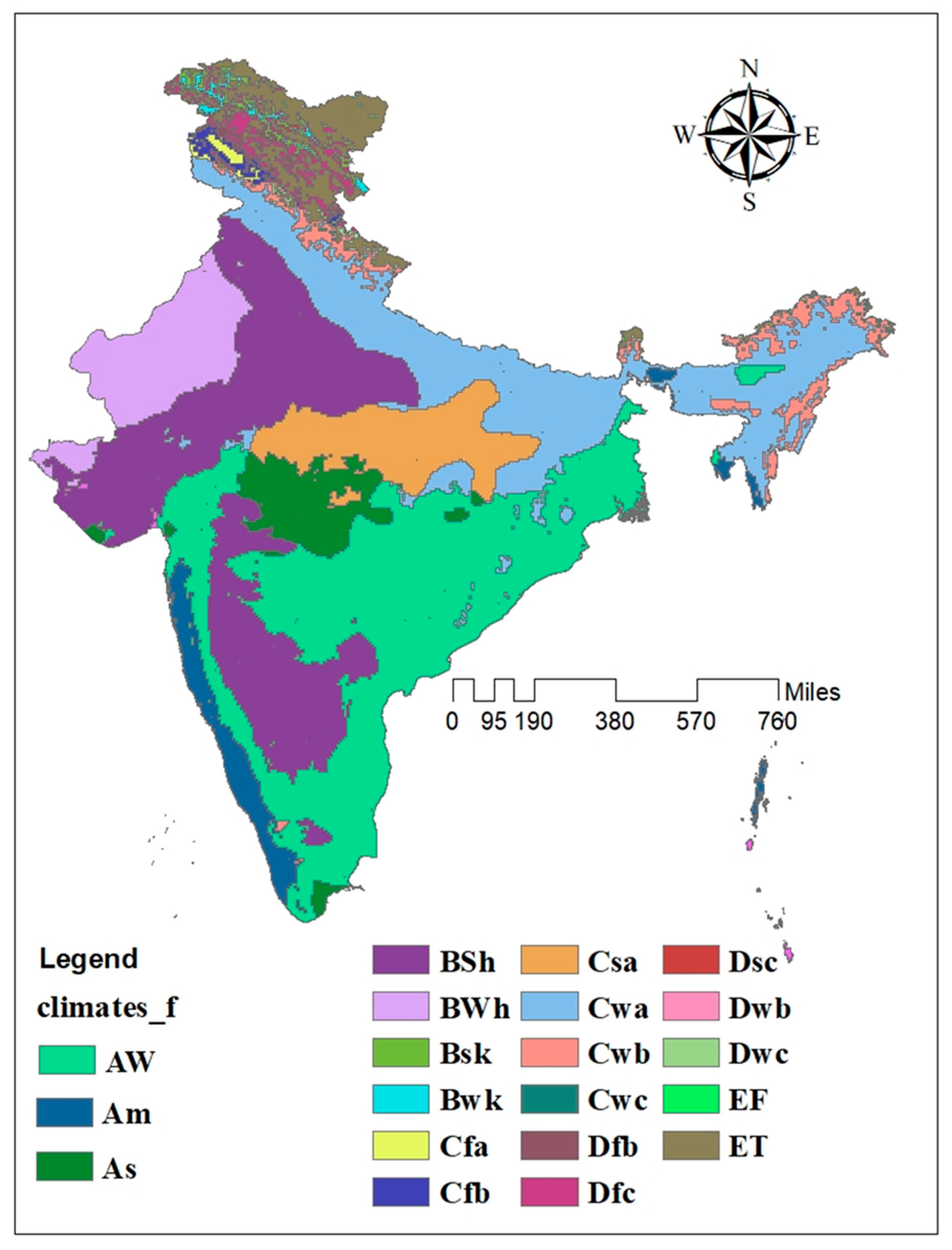
Figure 2. (a) Geographical location of selected stations in the Krishna River basin. (b) Precipitation Variability map and DEM of the Krishna River Basin.

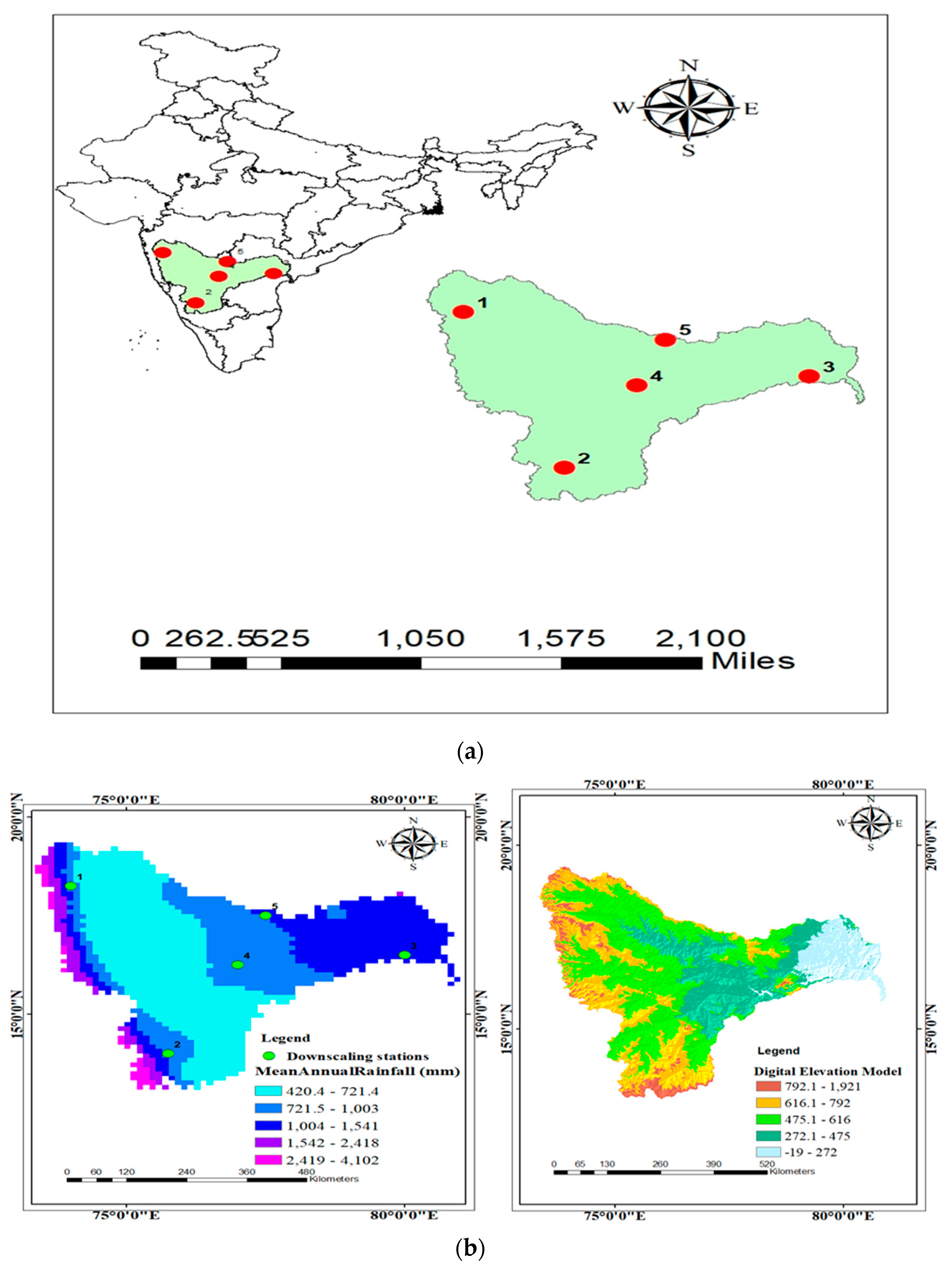
Figure 3. Schematic representation of Extreme learning machines.

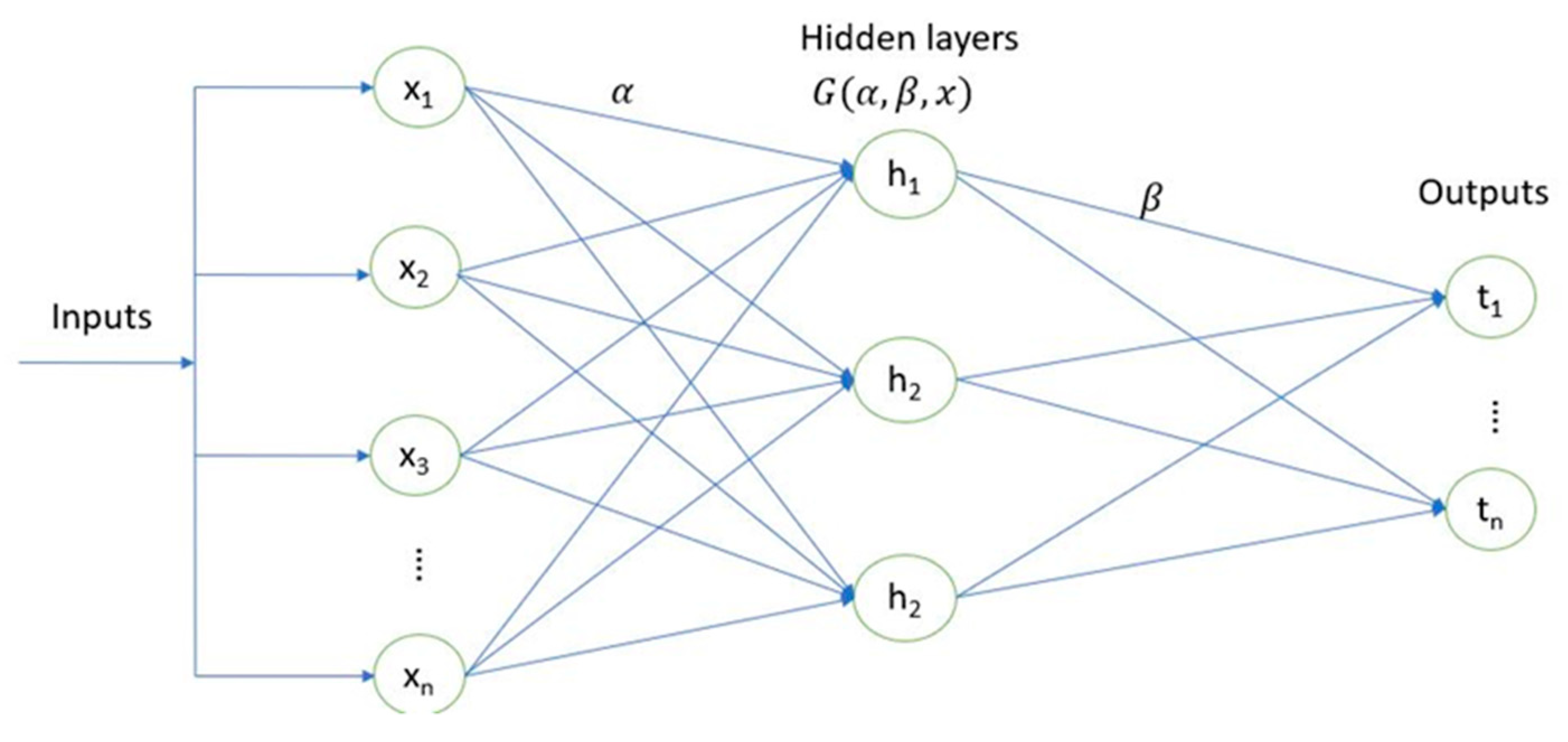
Figure 4. Sample Cross-correlation between different predictors and precipitation for the grid 2 (16.25N, 77E).

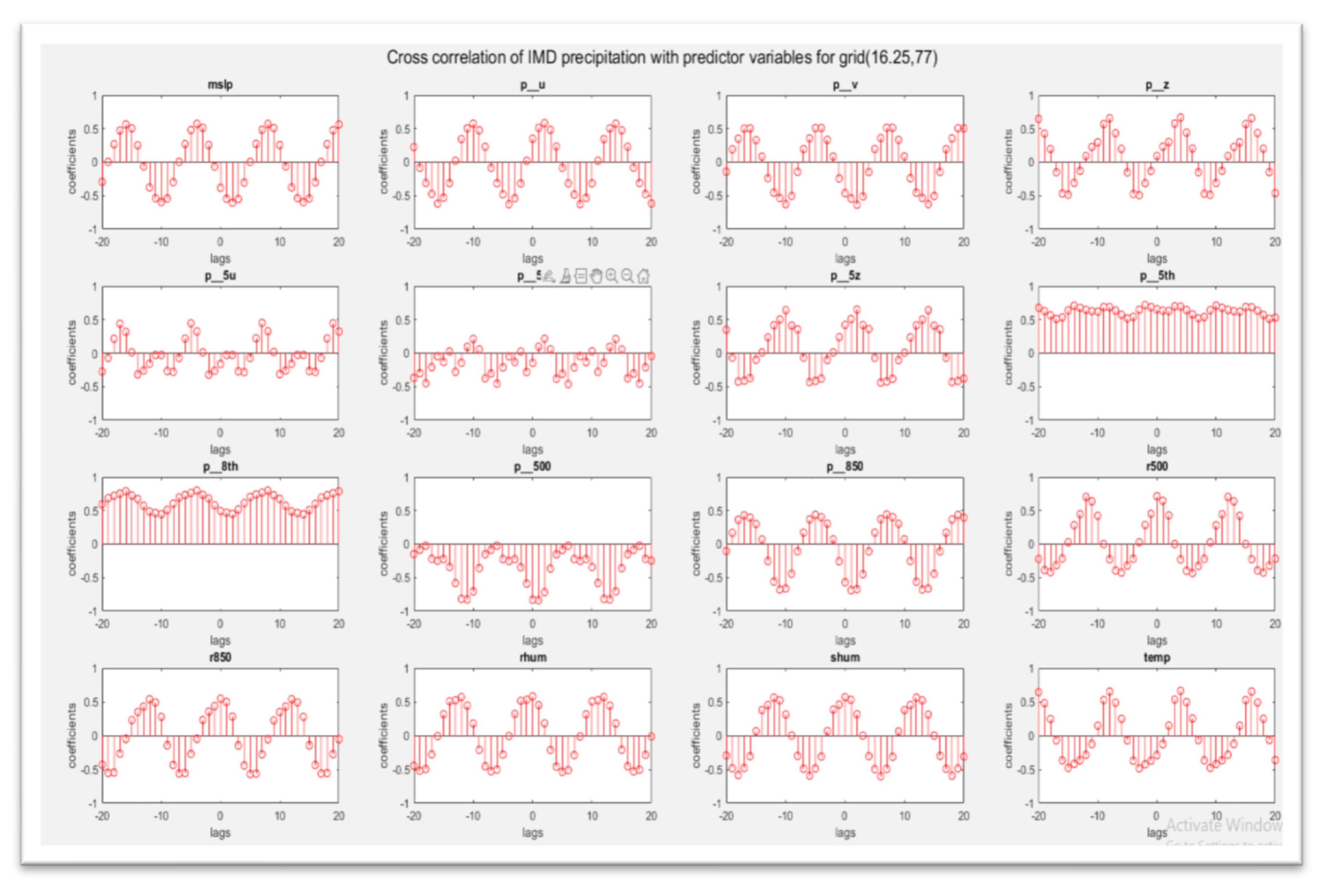
Table 1. Details of global and local predictor variables used for precipitation forecasting.

Level	Predictands
Global	Indian Oceanic Dipole (IOD) North Atlantic Oscillation (NAO) NINO Pacific Decadal Oscillation (PDO)
Local	Mean Sea level pressure (mslp) Zonal velocity component (p_u) Meridional velocity component (p_v) Vorticity (p_z) Specific humidity (shum) Relative humidity (rhum) Surface air temperature (temp) Zonal velocity component (p5_u) Meridional velocity component (p5_v) Vorticity (p5 _z) Wind direction (p5th) Geopotential height (p500) Relative humidity (r500) Wind direction (p8th) Geopotential height (p850) Relative humidity (r850)

Level

Predictands

Global

Indian Oceanic Dipole (IOD)
North Atlantic Oscillation (NAO)
NINO
Pacific Decadal Oscillation (PDO)

Local

Mean Sea level pressure (mslp)
Zonal velocity component (p_u)
Meridional velocity component (p_v)
Vorticity (p_z)
Specific humidity (shum)
Relative humidity (rhum)
Surface air temperature (temp)
Zonal velocity component (p5_u)
Meridional velocity component (p5_v)
Vorticity (p5 _z)
Wind direction (p5th)
Geopotential height (p500)
Relative humidity (r500) Wind direction (p8th)
Geopotential height (p850)
Relative humidity (r850)

Table 2. Results for various forecasting models for the Krishna River basin with global climate indices as inputs. The values for RMSE and MAE are normalized with respect to mean and standard deviation.

Station	MLR
Station	RMSE(mm)	Correlation	NSE	MAE(mm)
1	0.096	0.355	0.164	0.099
2	0.160	0.332	0.124	0.100
3	0.162	0.376	0.137	0.105
4	0.144	0.309	0.157	0.092
5	0.048	0.309	0.119	0.055
	FFBP-NN
1	0.090	0.694	0.481	0.058
2	0.091	0.680	0.458	0.063
3	0.092	0.669	0.446	0.065
4	0.063	0.730	0.529	0.032
5	0.052	0.713	0.504	0.036
	ELM
1	0.070	0.407	0.407	0.053
2	0.101	0.489	0.403	0.067
3	0.157	0.343	0.343	0.117
4	0.122	0.419	0.419	0.096
5	0.052	0.561	0.515	0.037
	WT FFBP-NN
1	0.111	0.598	0.385	0.077
2	0.106	0.644	0.403	0.075
3	0.113	0.572	0.385	0.078
4	0.113	0.567	0.391	0.078
5	0.108	0.636	0.383	0.080
	WT ELM
1	0.093	0.785	0.494	0.064
2	0.088	0.803	0.452	0.063
3	0.125	0.812	0.418	0.088
4	0.096	0.798	0.465	0.063
5	0.113	0.848	0.434	0.076

Table 3. Results for various forecasting models for the Krishna River basin with local predictor variables as inputs. The values for RMSE and MAE are normalized with respect to mean and standard deviation.

Station	MLR
Station	RMSE(mm)	Correlation	NSE	MAE(mm)
1	0.053	0.573	0.573	0.037
2	0.091	0.536	0.536	0.057
3	0.123	0.597	0.597	0.084
4	0.096	0.646	0.646	0.063
5	0.058	0.442	0.442	0.033
	FFBP-NN
1	0.055	0.545	0.545	0.038
2	0.086	0.576	0.576	0.054
3	0.012	0.600	0.600	0.078
4	0.092	0.678	0.678	0.058
5	0.062	0.713	0.362	0.031
	ELM
1	0.066	0.473	0.473	0.039
2	0.094	0.496	0.496	0.060
3	0.127	0.565	0.565	0.089
4	0.094	0.653	0.653	0.062
5	0.057	0.423	0.423	0.032
	WT FFBP-NN
1	0.109	0.771	0.556	0.069
2	0.082	0.779	0.549	0.057
3	0.084	0.753	0.505	0.063
4	0.061	0.787	0.563	0.041
5	0.070	0.765	0.520	0.052
	WT ELM
1	0.118	0.779	0.575	0.087
2	0.086	0.765	0.557	0.065
3	0.078	0.817	0.579	0.054
4	0.075	0.738	0.518	0.056
5	0.084	0.742	0.518	0.063

Table 4. Results for various forecasting models for the Krishna River basin with climate and local variables as inputs. The values for RMSE and MAE are normalized with respect to mean and standard deviation.

station	MLR
station	RMSE(mm)	Correlation	NSE	MAE(mm)
1	0.053	0.578	0.578	0.037
2	0.090	0.533	0.533	0.057
3	0.122	0.602	0.602	0.084
4	0.096	0.653	0.653	0.063
5	0.059	0.439	0.439	0.034
	FFBP-NN
1	0.050	0.616	0.616	0.035
2	0.083	0.604	0.604	0.049
3	0.108	0.691	0.691	0.069
4	0.087	0.714	0.714	0.053
5	0.052	0.5600	0.5600	0.032
	ELM
1	0.051	0.680	0.680	0.034
2	0.065	0.757	0.757	0.042
3	0.090	0.784	0.784	0.064
4	0.075	0.782	0.782	0.047
5	0.037	0.754	0.754	0.026
	WT FFBP-NN
1	0.083	0.892	0.741	0.055
2	0.072	0.849	0.648	0.052
3	0.077	0.784	0.595	0.056
4	0.061	0.802	0.636	0.036
5	0.064	0.820	0.591	0.042
	WT ELM
1	0.070	0.925	0.852	0.052
2	0.069	0.843	0.697	0.053
3	0.075	0.813	0.625	0.058
4	0.053	0.847	0.700	0.035
5	0.073	0.779	0.625	0.053

Table 5. Results of WT ELM models for India with combined global and local predictor variables. The values for RMSE and MAE are normalized with respect to mean and standard deviation.

Station	Central India
Station	RMSE(mm)	Correlation	NSE	MAE(mm)
1	0.0718	0.9084	0.8152	0.0059
2	0.0680	0.8751	0.7200	0.0491
3	0.0757	0.9260	0.8538	0.0584
4	0.0755	0.8775	0.7574	0.0567
	North India
1	0.0733	0.8437	0.7012	0.0537
2	0.0610	0.8864	0.7733	0.0447
3	0.0800	0.8286	0.6816	0.0581
4	0.0728	0.7804	0.5477	0.0554
	Peninsular
1	0.0927	0.8406	0.6619	0.0686
2	0.1009	0.7936	0.6112	0.0780
3	0.0419	0.9324	0.8580	0.0325
4	0.1030	0.8728	0.7602	0.0781
	Northwest
1	0.0784	0.9178	0.8401	0.0603
2	0.0628	0.8873	0.7437	0.0448
3	0.0802	0.7611	0.5025	0.0578
4	0.0696	0.8356	0.6765	0.0532

Table 6. Correlation between different climatic variables and precipitation with and without wavelet decomposition for Grid 2 (Dn indicates the decomposition and its level).

Climatic variable	Original scale	D1	D2	D3	D4	D5	D6	D7	D8	D9	D10
p5zas	0.011	0.011	0.051	0.061	0.061	0.081	0.161	0.361	0.421	0.271	0.121
p5th	0.131	0.001	-0.009	-0.019	-0.059	-0.069	-0.079	0.001	0.361	0.141	0.081
p8th	-0.019	0.001	0.001	0.011	0.001	-0.029	-0.159	-0.369	-0.409	-0.329	-0.109
rhum	0.111	0.021	0.031	0.061	0.121	0.201	0.331	0.401	0.361	0.331	0.171
shum	0.141	0.011	0.031	0.051	0.101	0.171	0.321	0.421	0.411	0.371	0.161
temp	0.071	-0.009	-0.019	-0.049	-0.099	-0.159	-0.199	-0.129	0.051	0.011	0.021
mslp	-0.079	-0.039	-0.079	-0.139	-0.169	-0.149	-0.239	-0.349	-0.389	-0.349	-0.099
uas	0.021	0.021	0.041	0.081	0.151	0.191	0.291	0.431	0.401	0.371	0.091
vas	-0.029	0.021	0.041	0.061	0.071	0.081	0.031	-0.269	-0.399	-0.319	-0.139
zas	0.171	0.011	0.221	0.021	0.021	0.021	0.001	0.021	0.071	0.041	0.031
p5 uas	-0.159	0.011	0.021	0.031	0.061	0.081	0.061	-0.029	-0.379	-0.179	-0.089
p5 vas	0.021	0.021	0.031	0.021	0.001	-0.019	-0.019	-0.109	-0.269	-0.089	-0.009
p500	0.091	-0.029	-0.069	-0.119	-0.149	-0.159	-0.209	-0.289	-0.369	-0.119	-0.009
p850	-0.059	-0.039	-0.089	-0.159	-0.199	-0.209	-0.359	-0.469	-0.439	-0.379	-0.089
r500	0.101	0.011	0.041	0.071	0.111	0.181	0.311	0.431	0.421	0.371	0.121
r850	0.051	0.021	0.041	0.071	0.141	0.211	0.321	0.411	0.351	0.301	0.141

# Values in bold show a significant correlation at 95% confidence levels.

Disclaimer/Publisher’s Note: The statements, opinions and data contained in all publications are solely those of the individual author(s) and contributor(s) and not of MDPI and/or the editor(s). MDPI and/or the editor(s) disclaim responsibility for any injury to people or property resulting from any ideas, methods, instructions or products referred to in the content.

© 2023 by the authors. Licensee MDPI, Basel, Switzerland. This article is an open access article distributed under the terms and conditions of the Creative Commons Attribution (CC BY) license (http://creativecommons.org/licenses/by/4.0/).

Copyright: This open access article is published under a Creative Commons CC BY 4.0 license, which permit the free download, distribution, and reuse, provided that the author and preprint are cited in any reuse.

MDPI Initiatives

Important Links

Choose an area of interest and we will send you notifications of new preprints at your preferred frequency.

Disclaimer

Development of Monthly Scale Precipitation Forecasting Model for Indian Subcontinent Using Wavelet Based Deep Learning Approach

Abstract

1. Introduction

2. Study Area and Data Used

3. Methods

3.1. Wavelet Transform (WT)

3.2. Extreme Learning Machines (ELM)

3.3. Wavelet Hybrid Models

4. Methodology

5. Results and Discussions

5.1. Forecasting using Single Scale Models

6. Conclusions

Author Contributions

Funding

Data Availability Statement

Acknowledgments

Conflicts of Interest

Appendix A

References

MDPI Initiatives

Important Links

Subscribe