
Submitted:
16 May 2023
Posted:
18 May 2023
You are already at the latest version
Abstract
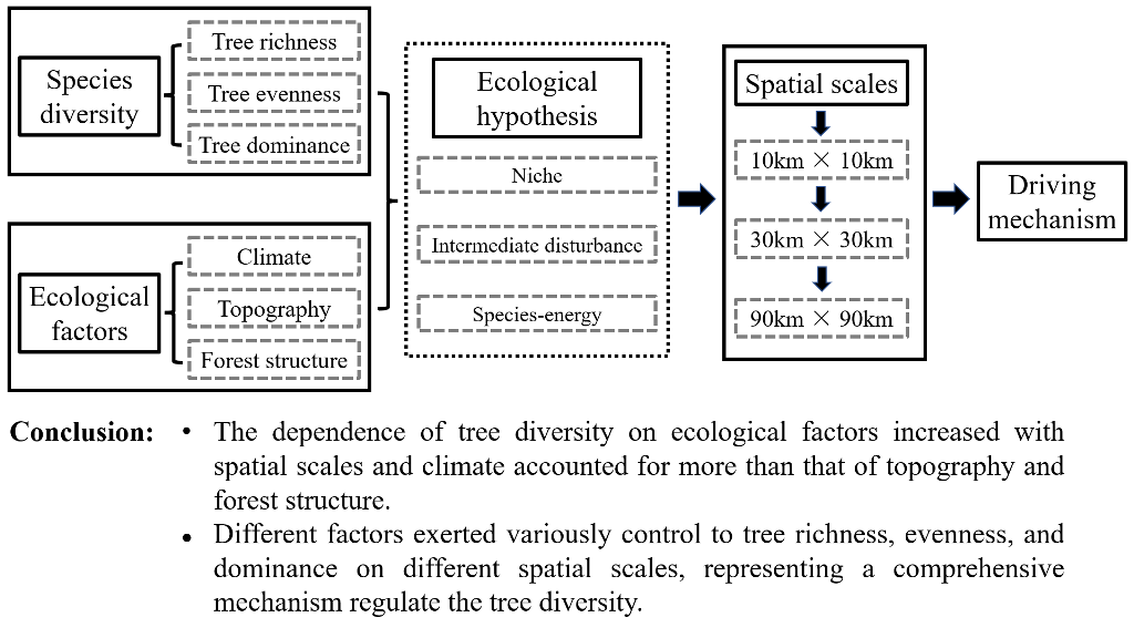
Species diversity has been shown to be influenced by environmental factors, but the mechanism underlying their relationship remains unclear across spatial scales. Based on field investigation data collected from 3,077 sample plots in temperate forest ecosystems, we compared tree species richness, evenness and dominance at 10 km × 10 km, 30 km × 30 km and 90 km × 90 km spatial scales. Then, we detected the scale dependence of changes in tree species composition on climate, topography and forest structure using variation partitioning and quantified their contribution to tree diversity with gradient boosted models (GBMs) and fitted their relationships. The magnitude of tree richness, evenness and dominance significantly increased with spatial scale. Ecological factors jointly accounted for 24.3%, 26.5% and 38.5% of the variation in tree species composition at the three spatial scales, respectively. Annual mean temperature had a strong impact on tree richness, evenness and dominance and peaked at an intermediate scale. Tree evenness and dominance increased with the variation of temperature but had upper and lower limits. Tree richness obviously increased with annual precipitation on multiple scales and decreased with annual sunshine duration at large spatial scale. Tree richness, evenness and dominance obviously increased with the variation elevation and diameter at breast height at large scales and small scales, respectively. Tree dominance decreased with tree height in a hump at small scale. The dependence of tree diversity on ecological factors increased with spatial scales. Furthermore, different factors exert various controls on tree diversity at different spatial scales, representing a comprehensive mechanism regulating tree diversity.
Keywords:
Biodiversity
; Tree richness
; Shannon index
; Simpson index
; Ecological mechanism
; Climate
; Topography
; Forest structure
1. Introduction
The dependence of biodiversity on spatial scale has long been a hot topic in ecology research [1,2,3,4]. Studying plant diversity at different spatial scales have great significance for understanding the spatial pattern of species diversity and its ecological drivers [5]. Given that the assembly mechanisms of communities vary across different spatial scales [1,6], diversity patterns at smaller spatial scales are usually different from those at larger scales [7,8,9,10,11]. However, there is still a lack of consensus regarding how ecological factors impact species diversity and drive its changes across different spatial scales.
Species diversity and environmental factors can be strongly scale-dependent, which presents a major obstacle to answering the above questions [4,12,13,14,15]. Climate, as one of the most important abiotic factors, has a strong impact on biodiversity across multiple spatiotemporal scales [3,6,16], and topographic factors, especially altitude, are thought to be more associated with diversity in montane regions [17]. Niche theory indicates that both biotic and abiotic interactions for living space and natural resources can promote the evolution rate and niche specialization, which tends to change with climatic gradient, especially temperature, through the kinetics of metabolism [18,19,20]. Species with broader niches can adapt to more abiotic conditions and tolerate a wider range of abiotic habitat changes and thus can disperse across larger geographic ranges [21]. In addition, latitude have strong impact on plant richness mainly by influencing the climate, such as temperature and precipitation [22,23,24]. Studies have shown that communities in warm, humid regions support more species than communities in cold, dry regions [25], while there is also evidence that adjacent areas with low temperature may have a higher biodiversity than areas with high temperature [26,27,28]. The intermediate disturbance hypothesis demonstrates that species diversity would likely peak at medium environmental gradients [29]; such as, plant species richness varying with altitude in a hump-type has been found in numerous taxa [7,26,30]. However, the variation in species-environment relationships across spatial scales is still unclear.
In contrast to the regional scale, the horizontal and vertical structure of forest, including the number and size of coexisting tree species individual in community, closely influences species diversity at the local scale by changing the energy distribution in the community [31]. The species-energy theory supposes that climate can strongly affect the primary productivity of plant, which mainly increases with temperature along latitudinal gradients, or the available energy partitioned into ecological systems [19,32,33]. On the one hand, more individuals can generally indicate higher species richness in statistics because 1) rare species may be more absent in smaller sample and 2) larger population sizes represent lower risk of extinction [32,33,34]. On the other hand, more tree abundance may not translate to higher species diversity [32,33] because available energy may also be distributed to maintain fewer higher/larger individuals rather than more. Disproportional species competition between larger/higher trees and smaller/shorter trees for limiting resources, such as sunshine, moisture or nutrients, can suppress plant diversity [35,36,37,38]. However, the effect of forest structure vs. climate and topography on species diversity varying with spatial scales remains unclear in temperate forests.
The mechanisms mentioned above are not mutually exclusive, but they may work together in explaining different aspects of biodiversity [31], such as species composition, richness, evenness (Shannon‒Wiener index) and dominance (Simpson index). Species composition represents the different species assembling in space; species richness, as the number of species, is the actuality of species assembling; species evenness, weighting species by their abundance, and species dominance, representing the relative percentage of species within an area, reflects community development under species assembly. Furthermore, comparing tree diversity among sites on a single spatial scale may yield unmatched results and hinder synthetic analyses [4,5], while multiple spatial scales are suitable for exploring complex ecological variations [39]. However, comprehensive tests on the relative contribution of ecological factors to various aspects of tree diversity across multiple spatial scales are infrequent.
The forest in Northeast China is one of the most species-rich area in temperate ecosystems. Vegetation surveying in this region over the past several years (2008-2016) has amassed sufficient data (3077 plots) for assessing the driving mechanisms of tree diversity across multiple spatial scales. In this study, we first compared patterns of tree diversity at three spatial scales, 10 km × 10 km, 30 km × 30 km and 90 km × 90 km. We then quantified the contributions of climatic, topographic and forest structure conditions to tree diversity. The primary aims of our study were to examine the variations in the ecological mechanisms driving tree diversity on different spatial scales. We investigated the following specific hypotheses about plant diversity in temperate forests: (1) the combined explanation of climate, topography and forest structure to tree composition increases with spatial scale, and climate has the largest contribution; (2) temperature mainly regulates tree evenness and dominance, and precipitation greatly influences tree richness on multiple spatial scales, but sunshine duration affects tree richness only on large spatial scales; (3) elevation obviously impacts tree richness, evenness and dominance at large spatial scales; and (4) the variation of diameter at breast height (DBH) can promote tree richness, evenness and dominance, but its effect decreases with an increasing spatial scale. We used species richness, the Shannon index and the Simpson index as primary measures of species diversity. Our study provides insights into the driving mechanisms of tree diversity patterns at multiple spatial scales.
2. Materials and Methods
2.1. Study Region and Sample Sites
This study concentrates on the natural mountain forests in Northeast China, mainly including 9 montane areas: Greater and Lesser Khingan, Zhangguangcailing, Wanda, Hadaling, Laoyeling, Longgang, Changbai, the western Liaoning mountains (Figure 1). The survey area extended from 39° N to 53° N and 116° E to 135° E, and this area has a temperate continental climate zone, with warm-rainy summers and cold-dry winters. The annual mean temperature varies from -6°C in the north to 11°C in the south. The most precipitation mainly occurs from June to September every year. The annual precipitation increases from 380 mm in the northwest to 1,130 mm in the southeast. The altitude ranges from 31 to 2115 m, and the slope varies from 0 to 46°. The forest types include mixed broad-leaved forest, mixed broadleaf-conifer forest, and coniferous forest [26].
In the summers of 2008 to 2016, we totally collected 3,077 sample plots, which had an area of 900 m2 (30 m×30 m). All the sample plots we investigated were natural forests far from roads and other human infrastructure. For the subsequent analysis, these plots served as the basic unit of the various grid scales. We recorded the geographic coordinates of the sampling center and measured the elevation (m) and slope (°) of each plot. Then, we conducted the surveys on the trees with diameter at breast height (DBH) ≥ 5 cm in each plot and standardized the tree species names based on the Flora of China (http://www.iplant.cn/foc). Finally, a total of 289,124 tree individuals including 155 tree species were collected. The number of tree species in the 3077 sample plots ranged from 1 to 21 (Figure S1).
2.2. Tree Diversity Scaling
Spatial representation and consistent approach for sampling plots at the local scale are crucial to the effective results about species diversity patterns and the dominant drivers at regional scales [11]. In this study, a sampling method executing contiguously arrayed grids such as the Scheiner’s Type II approach was used [40]. Comparing to the Scheiner's Type II approach, the main difference was that our examining grids were composed of the investigated 3077 sampling plots. First, we transformed the longitude and latitude (°) of the plots into geographic distance coordinates (km) on the plane with R package ‘geosphere’. Then, we divided the plane into 10 km ×10 km, 30 km × 30 km and 90 km × 90 km spatial scales of sampling grids, level by level (Figure S2), and then extracted the grid containing sample plots for subsequent statistical analysis. Finally, we obtained 615, 420 and 117 grids, which were the number of grids containing sample plots, at the three spatial scales, respectively.
In this study, the distribution of 3077 sampling plots were uneven covering the study area as shown in Figure 1. The tree diversity analysis could be potentially biased by the uneven sampling coverage. For example, we sampled more plots in the Changbai Mountains due to its higher species pool, and we sampled fewer plots in the Greater Khingan Mountains due to its lower species pool. To minimize this problem, we used a rarefaction and extrapolation approach to generate estimates of the tree diversity in each grid with the R package iNEXT [41]. Then, the 95% confidence intervals were calculated by the 0.025 and 0.975 quantiles with 1000 simulations of bootstrap samples. The simulated species richness, Shannon index and Simpson index values were the expected diversity.
2.3. Explanatory Variable Selection
We chose 9 variables to explain the variability in tree diversity, including climate, topography and forest structure (Table 1). We obtained standardized climate data, including the annual mean temperature (AMT, °C), annual precipitation (AP, mm) and annual sunshine duration (ASD, hour), with 500 m × 500 m resolution from the website of China Meteorological Administration (http://www.cma.gov.cn/). The climate data we used were averaged from 2008 to 2016, corresponding to the time of the plot survey. We selected three topographic factors, such as elevation (EL, m), slope (SL, °) and soil moisture index (SMI). As a function of topographic position and soil physicochemical properties, the SMI represents the capacity of soil holding water. In each grid, three easily measured and ecologically important forest structure variables were detected, including tree density (TD, the abundance of tree individuals per hectare), the diameter at breast height (DBH, cm) and tree height (TH, m). We calculated both the mean value and the coefficient of variation for the 9 variables in each grid, as the mean value may weaken the effect of the local conditions with increasing scale. Finally, we obtained 14 variables after excluding 4 collinear variables (r > 0.7), including AP cv, TWI cv, DBH mean and TH cv.
2.4. Data Analysis
These 14 variables, classified as climatic, topographic and forest structure conditions, were used for partitioning the total variation in tree diversity across Northeast China. We partitioned the explanatory variables into independent and shared components to analyze the three groups of predictors explaining the variation in tree species diversity. The ‘varpart’ function in vegan package based on linear regression was used to compute the adjusted R2 [42].
We fitted the gradient boosted models (GBMs) to detect the relative importance of predictors to tree diversity. The GBMs can provide accurate coefficients and reliable results, especially partitioning the correlation among predictive factors [43,44]. To minimize the influence of extreme outliers, the regression trees are gradually added, and data is reweighted to compensate for improper fitting of previous regression trees [24]. Therefore, the GBM can fit complex nonlinear relationships and realize higher accuracy and less bias without overfitting [45]. When fitting GBMs, we should specify two main parameters, including learning rate and tree complexity, which regulate the number and the interaction depth of regression trees, respectively [46]. We set 0.001 as learning rate value and 2 as tree complexity value. A Poisson distribution of errors was operated to match the response of tree richness to variables, as richness is the number of species [24]. The R package dismo and "gbm" scripts were used to examine the contribution of predictors. We detected the residuals of the GBMs for spatial independence with Moran’s I test and detected no statistically significant spatial autocorrelation; thus, we did not explore further. All descriptive statistic analyses were performed with R version 3.4.3 (http://www.r-project.org).
3. Results
3.1. Tree Diversity at Different Spatial Scales
The tree richness, Shannon index and Simpson index indicated the same variation in spatial patterns, and all increased with spatial scale (Figure 2). The analysis of variance showed that the tree richness, Shannon index and Simpson index at different spatial scales were significantly different (p ≤ 0.01).
3.2. Ecological Drivers of Tree Diversity
The measured ecological variables explaining the variation in tree species composition at the three spatial scales were 24.3%, 26.5% and 38.5%, respectively (Figure 3). Climatic factors explained the most independent fraction of tree diversity at the three grid scales (9.6%, 11.1% and 12.5%), but a small independent fraction was explained by topography (2.9%, 2.7% and 4.3%) and forest structure (4.2%, 3.9% and 5.0%). The combined explanations of the three components were 2.6%, 3.2% and 8.1%, respectively, with spatial scale.
The DBH cv influenced most on tree richness, and followed by AP mean and AMT mean, with relative contributions of 26.6%, 24.5% and 14.0% at the 10 km × 10 km spatial scale (Table 1). AP mean was strongest impact, followed by AMT mean and DBH cv, with relative contributions of 21.6%, 20.0% and 18.3% at the 30 km × 30 km spatial scale. AP mean contributed most, followed by ASD mean and EL cv, with relative contributions of 23.6%, 18.7% and 13.4% at the 90 km × 90 km spatial scale.
The DBH cv had the greatest impacted the Shannon index, followed by the AMT mean and AMT cv, with relative contributions of 31.6%, 23.7% and 9.3% at the 10 km × 10 km spatial scale (Table 1). AMT mean had the strongest influence, followed by DBH cv and AMT cv, with relative contributions of 30.2%, 20.3% and 14.3% at the 30 km × 30 km spatial scale. AMT cv contributed the most, followed by AMT mean and EL cv, with relative contributions of 28.7%, 28.1% and 16.4% at the 90 km × 90 km spatial scale.
For the Simpson index (Table 1), DBH cv had the greatest influence, followed by AMT mean and TH mean, with relative contributions of 23.6%, 20.9% and 10.1% at the 10 km × 10 km spatial scale. AMT mean was strongest impact, followed by AMT cv and DBH cv, with relative contributions of 22.2%, 16.9% and 13.1% at the 30 km × 30 km spatial scale. AMT cv contributed the most, followed by AMT mean and EL cv, with relative contributions of 46.7%, 19.7% and 15.2% at the 90 km × 90 km spatial scale.
In Figure 4, the three index of tree diversity responding to AMT mean and AMT cv had similar variation trends on different scales, but the extent of each was diverse. Tree richness changed with the AMT mean into a hump shape at the 10 km × 10 km and 30 km × 30 km scales but increased with the AMT mean and then smoothed at the 90 km × 90 km scale. Tree richness increased with AP mean, EL cv and DBH cv in an ascending ladder type. The changes of Shannon index and Simpson index with AMT mean, EL cv and DBH cv at the three scales were analogous to that of tree richness. The Shannon index increased with AMT cv and then smoothed, and the same with Simpson index. The Simpson index changed with the TH mean in a hump-shaped manner at the 10 km × 10 km scale but decreased with the TH mean in an ascending ladder type.
4. Discussion
To explore the underlying mechanism of biodiversity, we evaluated the contributions of climatic, topographic and forest structure factors to tree diversity at three spatial scales. We aimed to verify that the effect of these factors driving tree diversity was scale dependent. Our results showed that tree diversity of temperate forests in Northeast China was strongly affected by ecological factors across spatial scales (Figure 3) and various factors driving tree diversity at multiple spatial scales (Table 1).
The results showed that the strong dependence of tree species composition on ecological factors increased with spatial scale (Figure 4). Many studies have indicated that the patterns of species diversity had complex cross-scale effects on the environment [12,15,47]. One explanation is that large regions with high number of species could contain historically accumulated species which segregated by climate refuges [48] or survived in complex physiographical heterogeneity in small spaces [49]. This phenomenon would produce strong regional effect at large spatial scale, rather than at small scale [4]. In addition, plant diversity patterns indicate overlapping differences of the dispersal range of species [26,34], as species in different spaces have various demands for spatial resources and adaptabilities to the environment [50]. Thus, larger regions with more plant species have higher scale dependence on the environment. Our results indicated that climate has a stronger influence on tree diversity than topography and forest structure (Figure 3). Most studies have found that climate significantly impacts tree diversity across large regions, and the impact far exceeds the effects of other environmental factors [3,6,16,17,24,51], which is consistent with our study.
A positive relationship between tree diversity and annual mean temperature was found in our results (Figure 4). Study has shown that temperature drive species diversity across different spatial scales [52]. Chu et al. [31] suggested that regions with a less variable annual climate contain more tree species, which is not inconsistent with our results. Appropriate temperature variation can increase the temperature niche for tree species and maintain higher tree diversity. Niche theory demonstrates that the life history strategy of plant species is determined by their ecological and biological characteristics, and different approaches of utilizing natural resources are used by species via occupying their respective ecological niches [46,53]. This analysis supports niche theory and is consistent with our findings that temperature variation within the upper and lower limits has a positive effect on the evenness (Shannon index) and dominance (Simpson index) of tree species (Figure 4). We found that tree diversity responded to temperature in an obvious hump-type manner at the medium scale, which supports the intermediate disturbance hypothesis (IDH). As temperature represents energy, we analysed whether warmer regions may have stronger competition among canopy species and reduced tree diversity. Although this situation in warmer regions can lead to energy redundancy [26,54,55], it creates conditions for trees with higher energy utilization formed via evolution or niche specialization promoted by the kinetics of metabolism [18,19,20].
Tree richness exhibited significant positive relationships with increasing precipitation at different spatial scales (Figure 4), suggesting that wetter sites have higher richness than drier sites [26]. Studies have revealed that climate warming inclines to restrict species diversity in regions containing relatively scarce water resources [56], but increased precipitation can offset the negative effect [25]. The biophysical interaction between temperature and precipitation is not easily disentangled in studies of plant diversity at regional scale [57,58]. Furthermore, complex topography can affect the local water and energy budgets at small spatial scales and then indirectly drive distribution of plant species and the diversity patterns in a region [17,32,59]. However, precipitation contributes more to tree richness, while temperature contributes more to tree evenness and tree species dominance. This result reveals that community composition is greatly affected by precipitation, which is consistent with Zhang et al. [47], while the spatial distribution and development of communities are mainly regulated by temperature. This analysis simultaneously supports the species-energy theory and niche theory.
Sunshine duration had a pronounced negative effect on tree richness at large spatial scales (Figure 4). This may be because sites with high sunshine duration are located on ridges or at high elevations, where harsh environments, especially low temperatures, limit the survival of species [26]. Valleys and sites at low elevations tend to provide suitable microclimates and thus contain higher species diversity. We detected an obvious effect of elevation on tree diversity at large spatial scales (Table 1), which is consistent with other studies [2,60]. Our results showed that tree diversity increased with elevation variation but had an upper limit (Figure 4). This result indicated that greater topographic heterogeneity provides more habitat types and living spaces and improves tree diversification by promoting species to occupy different niches [61,62,63,64]. Furthermore, complex topography can create refuges for species that persist in adverse environmental conditions [5] and thus have more species.
A large DBH cv had a positive effect on diversity at small spatial scales (Table 1 and Figure 4). Trees occupying different spaces (horizontal and vertical) can improve community richness, evenness, and dominance because DBH cv represents the difference in the size of tree individuals, which is consistent with niche theory. We did not find a significant contribution of tree density to tree diversity, but there was a hump-type relationship between tree height and the Simpson index. The results showed that a moderate tree height could increase vertical space and promote diversity, but an excessive mean tree height in the community can reduce tree dominance by increasing competition among tree species. This analysis clearly supports the intermediate disturbance hypothesis and species-energy theory that states that available energy is distributed to support higher individuals, rather than more individuals, because of the suppression of tree diversity through asymmetric competition between taller trees and shorter trees for natural resources [35,36,37,38].
5. Conclusions
In conclusion, we found that a comprehensive mechanism regulates tree diversity in temperate forests. Changes in tree composition were strongly impacted by ecological factors, especially climate, which had the greatest contribution, and the effect increased with spatial scale. Temperature and precipitation could significantly promote tree diversity at multiple spatial scales. Temperature mainly regulated species evenness and dominance, while precipitation greatly affected species richness. Tree richness decreased with sunshine duration at large spatial scales. Tree diversity increased with large altitudinal heterogeneity, providing more survival habitat. Various individual sizes can improve tree diversity by occupying different niches, while excessive tree height of community can suppress tree dominance due to intense canopy competition.
Supplementary Materials
Additional supporting information may be found online in the Supporting Information section.
Author Contributions
Yue Gu: Methodology, Software, Writing - Original Draft, Writing - Review & Editing, Visualization; Junhui Zhang: Software, Data Curation, Funding acquisition; Wang Ma: Formal analysis, Writing - Review & Editing; Yue Feng: Formal analysis, Visualization; Leilei Yang: Formal analysis; Zhuo Li: Investigation; Yanshuang Guo: Investigation; Guoqiang Shi: Investigation; Shijie Han: Conceptualization, Validation, Data Curation, Supervision, Project administration, Funding acquisition.
Funding
This work was supported by the National Key Research and Development Program of China (No. 2016YFA0600804); Natural Science Foundation of Liaoning Province (No. 2019-BS-262); Academy of Changbai Mountain Science (No. 2017-03).
Data Availability Statement
The data presented in this study are available on request from the corresponding author. The data are not publicly available due to survey respondents were assured raw data would remain confidential.
Acknowledgments
We would like to thank Shihong Jia for providing language help and writing assistance.
Conflicts of Interest
The authors declare that they have no known competing financial interests or personal relationships that could have appeared to influence the work reported in this paper.
Author Biography: Yue Gu is a postdoctor at Qufu Normal University, Shandong, China. He interests in study of ecological and biogeographical processes that include forest biodiversity and its driving mechanism at multiple scales.
References
- Crawley, M.J.; Harral, J.E. Scale dependence in plant biodiversity. Science 2001, 291, 864–868. Available online: https://www.jstor.org/stable/3082397.
- Belmaker, J.; Jetz, W. Cross-scale variation in species richness-environment associations. Global Ecol. Biogeogr. 2011, 20, 464–474. [Google Scholar] [CrossRef]
- Malanson, G.P.; Fagre, D.B.; Zimmerman, D.L. Scale dependence of diversity in alpine tundra, Rocky Mountains, USA. Plant Ecol. 2018, 219, 999–1008. [Google Scholar] [CrossRef]
- Keil, P.; Chase, J.M. Global patterns and drivers of tree diversity integrated across a continuum of spatial grains. Nat. Ecol. Evol. 2019, 3, 390–399. [Google Scholar] [CrossRef] [PubMed]
- Stein, A.; Gerstner, K.; Kreft, H. Environmental heterogeneity as a universal driver of species richness across taxa, biomes and spatial scales. Ecol. Lett. 2014, 17, 866–880. [Google Scholar] [CrossRef]
- McGill, B.J. Matters of Scale. Science 2010, 328, 575–576. [Google Scholar] [CrossRef]
- Rahbek, C. The role of spatial scale and the perception of large-scale species-richness patterns. Ecol. Lett. 2005, 8, 224. [Google Scholar] [CrossRef]
- Chase, J.M.; Knight, T.M. Scale-dependent effect sizes of ecological drivers on biodiversity: Why standardised sampling is not enough. Ecol. Lett. 2013, 16, 17–26. [Google Scholar] [CrossRef]
- Cavieres, L.A.; Brooker, R.W.; Butterfield, B.J.; Cook, B.J.; Kikvidze, Z.; Lortie, C.J.; Callaway, R. M. Facilitative plant interactions and climate simultaneously drive alpine plant diversity. Ecol. Lett. 2014, 17, 193–202. [Google Scholar] [CrossRef]
- Gavilan, R.G.; Callaway, R.M. Effects of foundation species above and below tree line. Plant Biosyst. 2017, 151, 665–672. [Google Scholar] [CrossRef]
- Tuomisto, H.; Ruokolainen, K.; Vormisto, J.; Duque, A.; Sánchez, M.; Paredes, V. V.; Lähteenoja, O. Effect of sampling grain on patterns of species richness and turnover in Amazonian forests. Ecography 2017, 40, 840–852. [Google Scholar] [CrossRef]
- Hillebrand, H.; Blenckner, T. Regional and local impact on species diversity - from pattern to processes. Oecologia 2002, 132, 479–491. [Google Scholar] [CrossRef] [PubMed]
- Nogués-Bravo, D.; Araújo, M.B.; Romdal, T.; Rahbek, C. Scale effects and human impact on the elevational species richness gradients. Nature 2008, 453, 216–219. [Google Scholar] [CrossRef] [PubMed]
- Wang, X.; Fang, J.; Sanders, N.J.; White, P.S.; Tang, Z. Relative importance of climate vs local factors in shaping the regional patterns of forest plant richness across northeast China. Ecography 2009, 32, 133–142. [Google Scholar] [CrossRef]
- Zhang, X.; Wang, H.; Wang, R.; Wang, Y.; Liu, J. Relationships between plant species richness and environmental factors in nature reserves at different spatial scales. Pol. J. Environ. Stud. 2017, 26, 2375–2384. [Google Scholar] [CrossRef] [PubMed]
- Harrison, S.; Spasojevic, M.J.; Li, D. Climate and plant community diversity in space and time. Proc. Natl. Acad. Sci. USA 2020, 117. [Google Scholar] [CrossRef]
- Naud, L.; Msviken, J.; Freire, S.; Angerbjorn, A.; Dalen, L.; Dalerum, L. Altitude effects on spatial components of vascular plant diversity in a subarctic mountain tundra. Ecol. Evol. 2019, 9, 4783–4795. [Google Scholar] [CrossRef]
- Brown, J.H.; Gillooly, J.F.; Allen, A.P.; Savage, V.M.; West, G.B. Toward a metabolic theory of ecology. Ecology 2004, 85, 1771–1789. [Google Scholar] [CrossRef]
- Brown, J.H. Why are there so many species in the tropics? J. Biogeogr. 2014, 41, 8–22. [Google Scholar] [CrossRef]
- Sibly, R.M.; Brown, J.H.; Kodric-Brown, A. Metabolic Ecology: A Scaling Approach; Wiley-Blackwell, Oxford, 2012. [CrossRef]
- Gaston, K.J.; Chown, S.L. Why Rapoport’s Rule Does Not Generalise. Oikos 1999, 84, 309. [Google Scholar] [CrossRef]
- O’Brien, E.; Field, R.; Whittaker, R. Climatic gradients in woody plant (tree and shrub) diversity: Water-energy dynamics, residual variation, and topography. Oikos. 2000, 89, 588–600. [Google Scholar] [CrossRef]
- Wang, Z.; Fang, J.; Lin, T.X. Patterns, determinants and models of woody plant diversity in China. Proc. Biol. Sci. 2011, 278, 2122–2132. [Google Scholar] [CrossRef] [PubMed]
- Zhang, Y.; Chen, H.Y.H.; Taylor, A. Multiple drivers of plant diversity in forest ecosystems. Global Ecol. Biogeogr. 2014, 23, 885–893. [Google Scholar] [CrossRef]
- Cowles, J.; Boldgiv, B.; Liancourt, P.; Petraitis, P.S.; Casper, B.B. Effects of increased temperature on plant communities depend on landscape location and precipitation. Ecol. Evol. 2018, 8, 5267–5278. [Google Scholar] [CrossRef] [PubMed]
- Gu, Y.; Han, S.J.; Zhang, J.H.; Chen, Z.J.; Wang, W.J.; Feng, Y.; Jiang, Y.G.; Geng, S.C. Temperature-Dominated Driving Mechanisms of the Plant Diversity in Temperate Forests, Northeast China. Forests 2020, 11, 227. [Google Scholar] [CrossRef]
- Paudel, S.K.; Waeber, P.O.; Simard, S.W.; Innes, J.L.; Nitschke, C.R. Multiple factors influence plant richness and diversity in the cold and dry boreal forest of southwest Yukon, Canada. Plant Ecol. 2016, 217, 505–519. [Google Scholar] [CrossRef]
- Steinbauer, M.J.; Grytnes, J.A.; Jurasinski, G.; Kulonen, A.; Lenoir, J.; Pauli, H.; Wipf, S. Accelerated increase in plant species richness on mountain summits is linked to warming. Nature 2018, 556, 231. [Google Scholar] [CrossRef]
- Grime, J.P. Competitive exclusion in herbaceous vegetation. Nature 1973, 242, 344–347. [Google Scholar] [CrossRef]
- Rahbek, C. The elevational gradient of species richness: A uniform pattern? Ecography 1995, 18, 200–205. [Google Scholar] [CrossRef]
- Chu, C.; Lutz, J.A.; Král, K.; Vrška, T.; Yin, X.; Myers, J. A.; Burslem, D.F.R.P. Direct and indirect effects of climate on richness drive the latitudinal diversity gradient in forest trees. Ecol. Lett. 2019, 22, 245–255. [Google Scholar] [CrossRef]
- Currie, D.J.; Mittelbach, G.G.; Cornell, H.W.; Field, R.; Guegan, J.F.; Hawkins, B.A.; Turner, J.R.G. Predictions and tests of climate-based hypotheses of broad-scale variation in taxonomic richness. Ecol. Lett. 2004, 7, 1121–1134. [Google Scholar] [CrossRef]
- Storch, D.; Bohdalková, E.; Okie, J. The more-individuals hypothesis revisited: The role of community abundance in species richness regulation and the productivity-diversity relationship. Ecol. Lett. 2018, 21, 920–937. [Google Scholar] [CrossRef] [PubMed]
- O'Brien, E.M. Water-energy dynamics, climate, and prediction of woody plant species richness: An interim general model. J. Biogeogr. 1998, 25, 379–398. [Google Scholar] [CrossRef]
- Franklin, J.F.; Spies, T.A.; Pelt, R.V.; Carey, A.B.; Thornburgh, D.A.; Berg, D.R.; Chen, J. Disturbances and structural development of natural forest ecosystems with silvicultural implications, using Douglas-fir forests as an example. Forest Ecol. Manag. 2002, 155, 399–423. [Google Scholar] [CrossRef]
- Coomes, D.A.; Lines, E.R.; Allen, R.B. Moving on from Metabolic Scaling Theory: Hierarchical models of tree growth and asymmetric competition for light. J. Ecol. 2011, 99, 748–756. [Google Scholar] [CrossRef]
- Lutz, J.A.; Larson, A.J.; Furniss, T.J.; Donato, D.C.; Freund, J.A.; Swanson, M.E. Spatially nonrandom tree mortality and ingrowth maintain equilibrium pattern in an old-growth Pseudotsuga-Tsuga Forest. Ecology 2014, 95, 2047–2054. [Google Scholar] [CrossRef] [PubMed]
- Farrior, C.E.; Bohlman, S.A.; Hubbell, S.; Pacala, S.W. Dominance of the suppressed: Power-law size structure in tropical forests. Science 2016, 351, 155–157. [Google Scholar] [CrossRef]
- Li, Z.; Han, H.; You, H.; Cheng, X.; Wang, T. Effects of local characteristics and landscape patterns on plant richness: A multi-scale investigation of multiple dispersal traits. Ecol. Indic. 2020, 117, 106584. [Google Scholar] [CrossRef]
- Scheiner, S.M. Six types of species-area curves. Global Ecol. Biogeogr. 2003, 12, 441–447. [Google Scholar] [CrossRef]
- Hsieh, T.C.; Ma, K.H.; Chao, A. iNEXT: iNterpolation and EXTrapolation for species diversity. R package, Version 3.0.0, 2022. Available online: http://chao.stat.nthu.edu.tw/wordpress/software_download/ (accessed on 13 October 2022).
- Oksanen, J.; Blanchet, F.G.; Kindt, R.; Legendre, P.; Minchin, P.R.; O’Hara, R.B.; Wagner, H. Vegan: Community ecology package. R package, Version 2.6-4, 2022. Available online: http://CRAN.R-project.org/package=vegan (accessed on 11 October 2022).
- Friedman, J.H. Greedy function approximation: A gradient boosting machine. Ann. Stat. 2001, 29, 1189–1232. [Google Scholar] [CrossRef]
- Leathwick, J.R.; Elith, J.; Francis, M.P.; Hastie, T.; Taylor, P. Variation in demersal fish species richness in the oceans surrounding New Zealand: An analysis using boosted regression trees. Mar. Ecol. Prog. Ser. 2006, 321, 267–281. [Google Scholar] [CrossRef]
- Elith, J.; Graham, C.H.; Anderson, R.P.; Dudik, M.; Ferrier, S.; Guisan, A.; Zimmermann, N.E. Novel methods improve prediction of species' distributions from occurrence data. Ecography 2006, 29, 129–151. [Google Scholar] [CrossRef]
- Connell, J.H. Diversity in tropical rain forests and coral reefs - High diversity of trees and corals is maintained only in a nonequilibrium state. Science 1978, 199, 1302–1310. [Google Scholar] [CrossRef] [PubMed]
- Zhang, C.; He, F.; Zhang, Z.; Zhao, X.; Gadow, K.V. Latitudinal gradients and ecological drivers of beta-diversity vary across spatial scales in a temperate forest region. Global Ecol. Biogeogr. 2020, 29, 1257–1264. [Google Scholar] [CrossRef]
- Svenning, J.-C.; Skov, F. Limited filling of the potential range in European tree species. Ecol. Lett. 2004, 7, 565–573. [Google Scholar] [CrossRef]
- Qian, H.; Ricklefs, R.E. Large-scale processes and the Asian bias in species diversity of temperate plants. Nature 2000, 407, 180–182. [Google Scholar] [CrossRef]
- Gao, D.; Perry, G. Detecting the small island effect and nestedness of herpetofauna of the West Indies. Ecol. Evol. 2016, 6, 5390–5403. [Google Scholar] [CrossRef] [PubMed]
- Qian, H.; Kissling, W.D. Spatial scale and cross-taxon congruence of terrestrial vertebrate and vascular plant species richness in China. Ecology 2010, 91, 1172–1183. [Google Scholar] [CrossRef] [PubMed]
- Schweiger, A.H.; Beierkuhnlein, C. Scale dependence of temperature as an abiotic driver of species' distributions. Global Ecol. Biogeogr. 2016, 25, 1013–1021. [Google Scholar] [CrossRef]
- Silvertown, J. Plant coexistence and the niche. Trends Ecol. Evol. 2004, 19, 605–611. [Google Scholar] [CrossRef]
- Chen, S.B.; Jiang, G.M.; OUYANG, Z.Y.; Xu, W.H.; Xiao, Y. Relative importance of water, energy, and heterogeneity in determining regional pteridophyte and seed plant richness in China. J. Syst. Evol. 2011, 49, 95–107. [Google Scholar] [CrossRef]
- Currie, D.J. Energy and Large-Scale Patterns of Animal- and Plant-Species Richness. Am. Nat. 1991, 137, 27–49. [Google Scholar] [CrossRef]
- Pfeifer-Meister, L.; Bridgham, S.D.; Reynolds, L.L.; Goklany, M.E.; Wilson, H.E.; Little, C.J.; Ferguson, A.; Johnson, B.R. Climate change alters plant biogeography in Mediterranean prairies along the West Coast, USA. Global Change Biol. 2016, 22, 845–855. [Google Scholar] [CrossRef] [PubMed]
- Kikvidze, Z.; Michalet, R.; Brooker, R.W.; Cavieres, L.A.; Lortie, C.J.; Pugnaire, F.I.; Callaway, R.M. Climatic drivers of plant-plant interactions and diversity in alpine communities. Alpine Bot. 2011, 121, 63–70. [Google Scholar] [CrossRef]
- Peyre, G.; Balslev, H.; Font, X.; Tello, J. S. Fine-Scale Plant Richness Mapping of the Andean Paramo According to Macroclimate. Front. Ecol. Evol. 2019, 7, 1–12. [Google Scholar] [CrossRef]
- Yu, F.; Wang, T.; Groen, T.A.; Skidmore, A.K.; Yang, X.; Geng, Y.; Ma, K. Multi-scale comparison of topographic complexity indices in relation to plant species richness. Ecol. Complex. 2015, 22, 93–101. [Google Scholar] [CrossRef]
- Rahbek, C.; Graves, G. R. Multiscale assessment of patterns of avian species richness. Proc. Natl. Acad. Sci. USA 2001, 98, 4534–4539. [Google Scholar] [CrossRef]
- Fernandez-going, B.M.; Harrison, S.P.; Anacker, B.L.; Safford, H.D. Climate interacts with soil to produce beta diversity in Californian plant communities. Ecology 2013, 94, 2007–2018. [Google Scholar] [CrossRef]
- Harrison, S.; Cornell, H. Toward a better understanding of the regional causes of local community richness. Ecol. Lett. 2008, 11, 969–979. [Google Scholar] [CrossRef]
- Kallimanis, A.S.; Mazaris, A.D.; Tzanopoulos, J.; Halley, J.M.; Pantis, J.D.; Sgardelis, S.P. How does habitat diversity affect the species-area relationship? Global Ecol. Biogeogr. 2008, 17, 532–538. [Google Scholar] [CrossRef]
- Quintero, I.; Jetz, W. Global elevational diversity and diversification of birds. Nature 2018, 555, 246–250. [Google Scholar] [CrossRef]
Figure 1.
Distribution of the 3,077 sampling plots in northeast China.
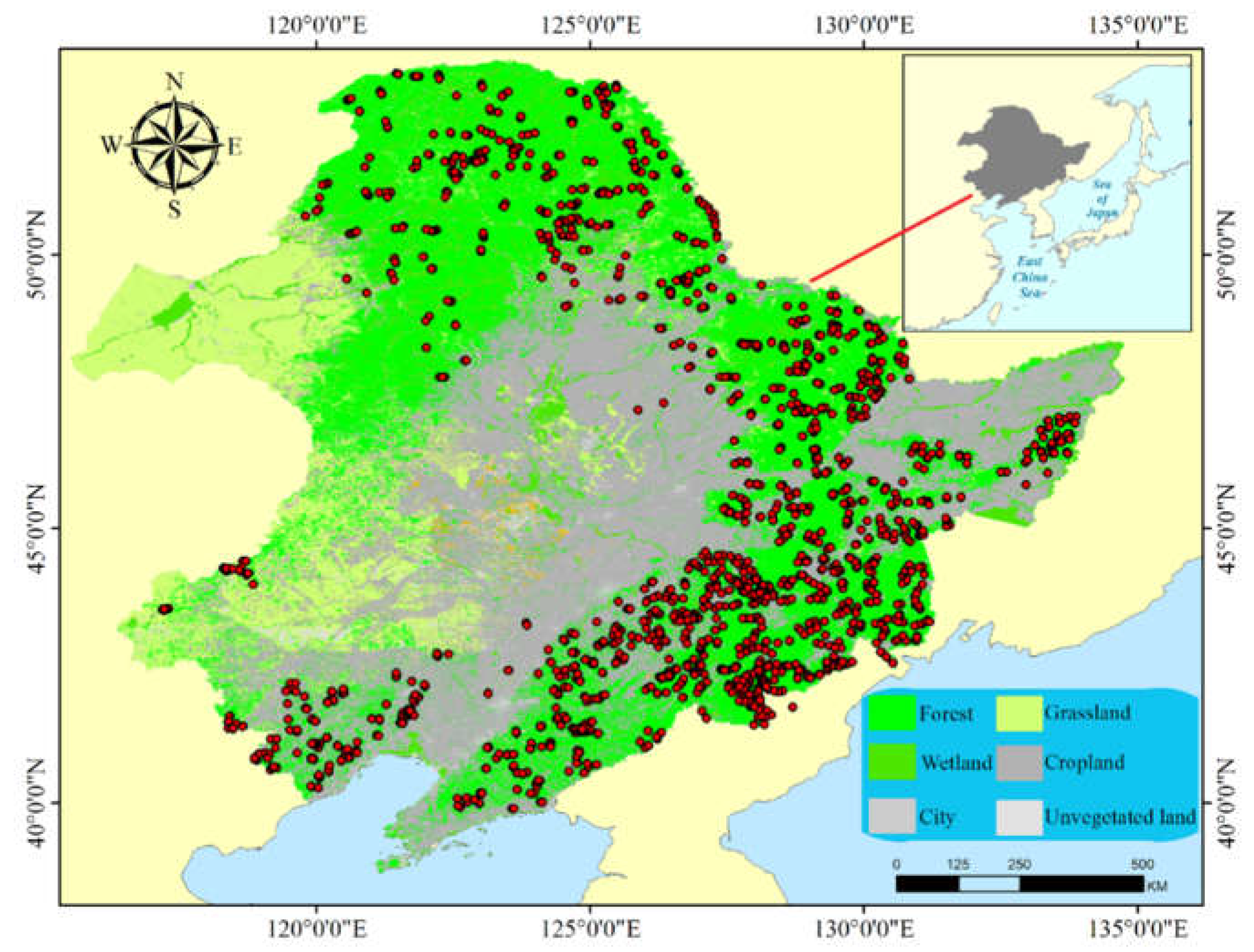
Figure 2.
Box plots showing the variation in tree diversity at different grid scales. (1) Tree richness, (2) Shannon index, (3) Simpson index. The letters a, b and c indicate significant differences among spatial scales for a given diversity index.
Figure 2.
Box plots showing the variation in tree diversity at different grid scales. (1) Tree richness, (2) Shannon index, (3) Simpson index. The letters a, b and c indicate significant differences among spatial scales for a given diversity index.
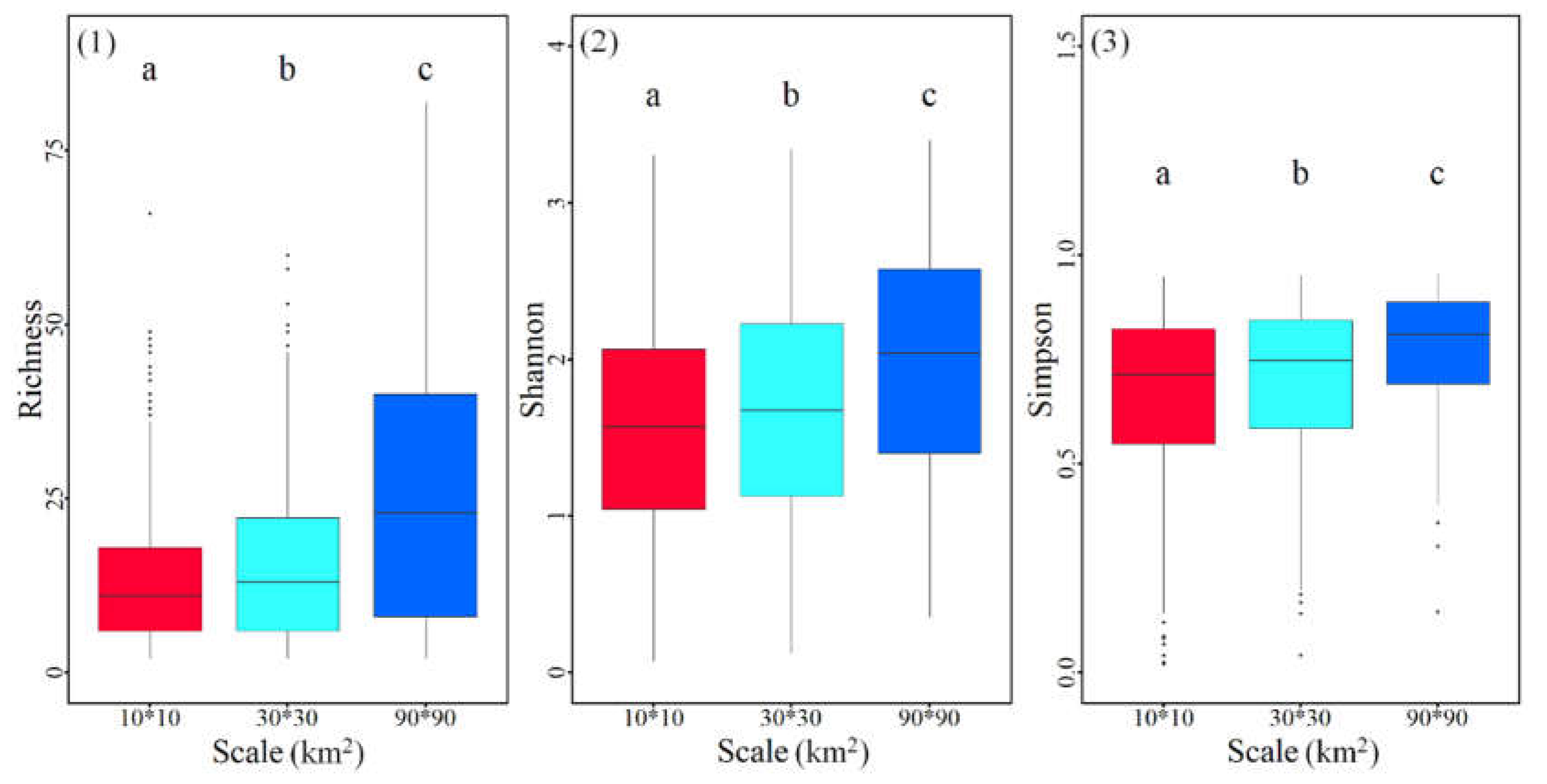
Figure 3.
Venn diagrams indicating the variation partitioning of tree species diversity explained by climate (X1), topography (X2) and forest structure (X3). The numbers in the diagrams represent the R2 values explained by ecological variables. The histograms are the total explained proportion of the diversity variation. (1) 10 km × 10 km grid scale, (2) 30 km × 30 km grid scale, and (3) 90 km × 90 km grid scale.
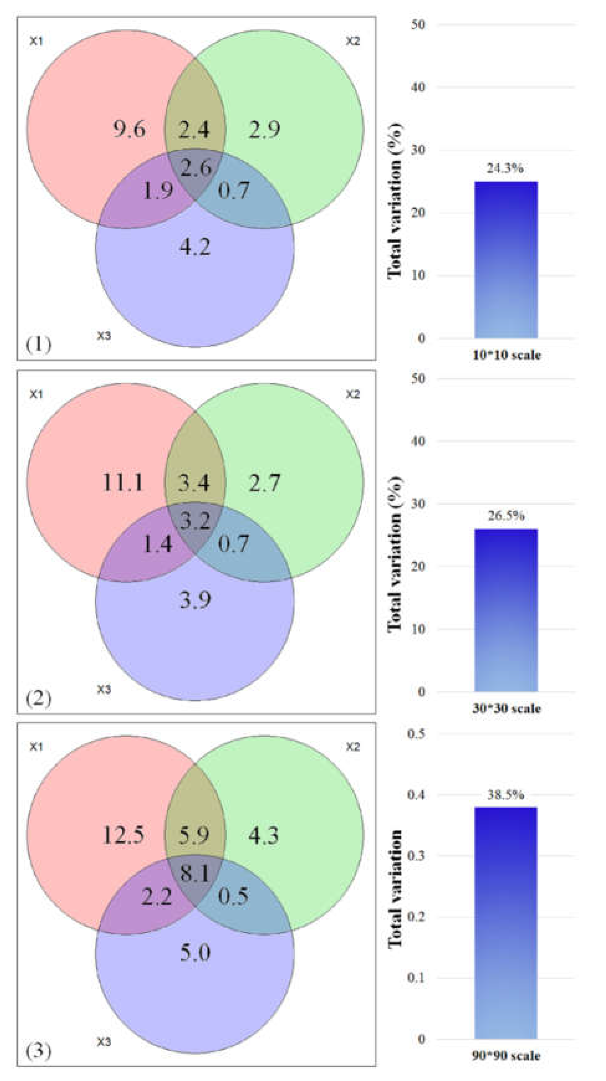
Figure 4.
The relationships between tree species diversity and predictors at three spatial scales. (1) Tree richness; (2) Shannon index; (3) Simpson index. AMT, annual mean temperature; AP, annual precipitation; ASD, annual sunshine duration; EL, elevation; DBH, diameter at breast height; TH, tree height.
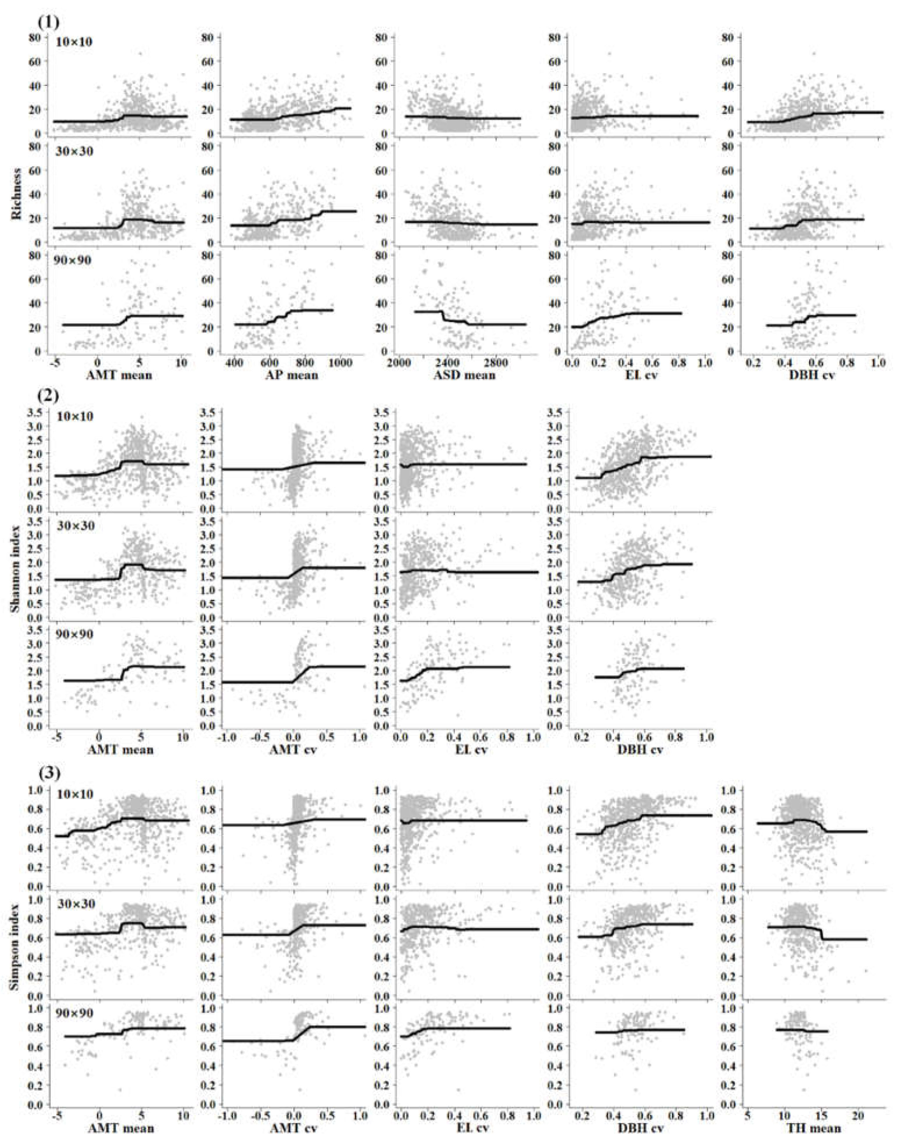

Table 1.
The contribution of ecological variables (%) to tree diversity fitted in GBM.
| Variables | Richness | Shannon | Simpson | ||||||
| 10*10 | 30*30 | 90*90 | 10*10 | 30*30 | 90*90 | 10*10 | 30*30 | 90*90 | |
| AMT mean | 14.0 | 20.0 | 11.7 | 23.7 | 30.2 | 28.1 | 20.9 | 22.2 | 19.7 |
| AMT cv | 13.3 | 10.1 | 10.6 | 9.3 | 14.3 | 28.7 | 8.1 | 16.9 | 46.7 |
| AP mean | 24.5 | 21.6 | 23.6 | 8.2 | 7.4 | 4.3 | 6.4 | 5.1 | 3.3 |
| ASD mean | 4.8 | 4.4 | 18.7 | 2.6 | 2.2 | 3.3 | 2.6 | 2.2 | 1.0 |
| ASD cv | 0.9 | 7.9 | 2.0 | 0.3 | 2.9 | 2.5 | 0.2 | 1.2 | 1.1 |
| EL mean | 2.5 | 2.9 | 2.5 | 3.8 | 2.4 | 0.7 | 2.6 | 3.8 | 0.1 |
| EL cv | 2.4 | 2.6 | 13.4 | 3.1 | 2.1 | 16.4 | 4.8 | 4.4 | 15.2 |
| SL mean | 0.5 | 2.9 | 0.3 | 1.6 | 1.8 | 0.5 | 2.7 | 3.9 | 1.5 |
| SL cv | 3.3 | 1.2 | 3.0 | 1.4 | 1.6 | 1.9 | 3.5 | 1.4 | 0.6 |
| TWI mean | 0.5 | 1.3 | 0.4 | 1.3 | 2.5 | 0.4 | 2.4 | 4.4 | 0.8 |
| TD mean | 2.8 | 3.0 | 2.9 | 2.5 | 5.5 | 3.3 | 3.4 | 6.5 | 3.1 |
| TD cv | 2.7 | 3.1 | 0.9 | 5.6 | 4.3 | 0.9 | 8.8 | 6.6 | 2.9 |
| DBH cv | 26.6 | 18.3 | 9.6 | 31.6 | 20.3 | 7.8 | 23.6 | 13.1 | 2.4 |
| TH mean | 1.2 | 0.7 | 0.6 | 4.9 | 2.5 | 1.3 | 10.1 | 8.3 | 1.6 |
| Distribution | Poisson | Poisson | Poisson | Gaussian | Gaussian | Gaussian | Gaussian | Gaussian | Gaussian |
| TC | 2 | 2 | 2 | 2 | 2 | 2 | 2 | 2 | 2 |
| LR | 0.001 | 0.001 | 0.001 | 0.001 | 0.001 | 0.001 | 0.001 | 0.001 | 0.001 |
| R2 | 0.65 | 0.77 | 0.85 | 0.69 | 0.80 | 0.86 | 0.62 | 0.73 | 0.69 |
Note: AMT, annual mean temperature; AP, annual precipitation; ASD, annual sunshine duration; EL, elevation; SL, slope; SMI, soil moisture index; TD, tree density; DBH, diameter at breast height; TH, tree height; TC, tree complexity, LR, learning rate. Bold numbers indicate the top three impacts of environmental factors on tree diversity.
Disclaimer/Publisher’s Note: The statements, opinions and data contained in all publications are solely those of the individual author(s) and contributor(s) and not of MDPI and/or the editor(s). MDPI and/or the editor(s) disclaim responsibility for any injury to people or property resulting from any ideas, methods, instructions or products referred to in the content. |
© 2023 by the authors. Licensee MDPI, Basel, Switzerland. This article is an open access article distributed under the terms and conditions of the Creative Commons Attribution (CC BY) license (http://creativecommons.org/licenses/by/4.0/).
Copyright: This open access article is published under a Creative Commons CC BY 4.0 license, which permit the free download, distribution, and reuse, provided that the author and preprint are cited in any reuse.


