This paper introduces a method to achieve optimal Gaussian estimation even when operating with low precision numerical representations of the full covariance matrix, such as 16-bit integer or 32-bit single precision formats, instead of more expensive double precision floating point representations (64 bits). The approximation's numerical error is accurately estimated in a conservative manner, resulting in minimal covariance inflation. When combined with a compressed estimator like the GCKF (Global Compressed Kalman Filter), which performs global updates at low frequency, this approach produces estimates that are nearly identical to the optimal ones. The deviation between the results obtained using this new approach and those obtained with the standard GCKF (which operates in double precision) is negligible. This new method is particularly relevant in high-dimensional estimation problems that require high-frequency operation. By leveraging the compressed operation of the GCKF, the estimation process applies the necessary approximation only during low-frequency global updates, using the single precision format instead of the more expensive double precision representations. The introduced numerical approximation is accurately estimated while maintaining a conservative approach, resulting in minimal covariance inflation. When combined with the GCKF, which performs global updates at low frequency, the estimates produced are almost identical to the optimal ones. This approach is particularly useful in high-dimensional estimation problems that require high-frequency operation. By representing the full covariance matrix in a low precision numerical format and applying appropriate scaling, memory usage is significantly reduced, offering substantial benefits for high-dimensional estimation problems and enabling real-time smoothing processes in such cases. By reducing the memory requirements for storing the full covariance matrix, the CPU avoids encountering a high number of page faults, resulting in improved processing performance. Lastly, the experimental section verifies the performance of the proposed approach in a single precision (32-bit floating point) GCKF SLAM process, assessing expected values and standard deviations of marginal PDFs.

Keywords:

Subject: Engineering - Electrical and Electronic Engineering

1. Introduction

The Bayesian estimation of the state of high dimensional systems is a relevant topic in diverse research and application areas. When a Gaussian estimator is applied in an optimal way, the full covariance matrix needs to be maintained during the estimation process; for that, the numerical format commonly used for representing the elements of the covariance matrix is double precision floating point (e.g. the 64 bits IEEE-754) or, in some cases, in which the covariance matrix characteristic allows it, single precision floating point (32 bits IEEE-754). However, in certain cases, single precision can result in numerical problems. Numerical formats of even lower precision, e.g., 16 bits, are usually more difficult to be applied, due to usual numerical instability, lack of consistence or, in the best cases where the approximation is properly applied (by performing matrix inflation), highly conservative results. However, when properly treated, a full Gaussian filter can operate in low precision without incurring in relevant errors or in excessive conservativeness. In particular, for systems that can be processed through a Generalized Compressed Kalman Filter (GCKF) [1], it is possible to operate under lower precision numerical format. The advantage of maintaining and storing the huge covariance matrix using low precision is relevant because the required memory can be reduced to a fraction of the nominal required amount. In addition to reducing the amount of required data memory, the fact that a program operates using lower amount of memory, improves its performance by incurring in lower numbers of RAM cache misses, a limitation which is still present in the current computer technology. This effect is even more relevant when those operations do occur at high frequency. That is the case of a standard Gaussian estimator performing update steps, because those imply updating the full covariance matrix, which means the full covariance matrix is read and written at each KF update, i.e., all the elements of the covariance matrix are R/W acceded. If, in addition to the high dimensionality and high frequency operation, the estimation process involves the capability of performing smoothing, then the requirements of memory can be dramatically increased, further exacerbating the problem.

The approach presented in this paper exploits the low frequency nature of the global updates of the GCKF in combination with a simple matrix decorrelation technique, for treating truncation errors associated to low precision numerical representation. Only during the low frequency global updates, the full covariance matrix is modified. That particularity of the GCKF allows performing additional processing on the full covariance matrix, if required for diverse purposes. As the global updates are performed at low execution rate, the cost of the treatment of the full covariance matrix is amortized over the overall operation, in many cases making the overhead result in very low extra cost. One of the purposes of treating the full covariance matrix,

P

, can be for approximating it by a low precision version of it; e.g. for representing the covariance matrix in single precision format or even by lower precision representations such as scaled 16 bit integers. Just truncating precision (truncating bits) is not adequate for replacing a covariance matrix; consequently, proper relaxation of the matrix needs to be performed. One way of doing it is by generating a bounding matrix,

P^{*}

, which satisfies two conditions:

1) The approximating matrix,

P^{*}

, must be more conservative that the original one (the one being approximated), i.e.

P^{*} - P

must be positive semidefinite; this fact is usually expressed as

P^{*} - P \geq 0

or as

P^{*} \geq P

P^{*}

is represented through a lower precision format.

In addition, it is desirable that the discrepancy

P^{*} - P

should be as small as possible to avoid over conservative estimates, particularly if the approximation needs to be applied repeatedly. This technique would allow a GCKF engine to operate servicing a number of clients, that when request a global update to be performed, the required memory for temporary storing and processing the full covariance matrix is partially or fully provided by the engine, while the memory for storing the low precision version of the full covariance matrixes is maintained by the clients, which means that the actual required memory for double precision is only one and it is shared by many client processes.

In addition, the required precision can be dynamically decided according to the availability of memory resources, observability of the estimation process and required accuracy of the estimates. The technique would also allow to maintain copies of the full covariance matrix at different times (regressors of matrixes), e.g., for cases of smoothing.

2. The Generalized Compressed Kalman filter (GCKF)

The GCKF is the approach introduced in [1]. The approach is intended to process estimations problems in high dimensional cases, in which the state vector is composed by hundreds or thousands of scalar components. Those estimation processes may need to operate at high processing rates for systems whose dynamics is fast and high dimensional, such as certain Stochastic Partial Differential Equations (SPDE), and also for certain Simultaneous Localization and Mapping (SLAM) applications.

The GCKF divides the estimation process in a low-frequency global component (a high dimensional Gaussian PDF which is updated at a low rate, called the “global component” of the estimation process). In addition to that, the estimation process maintains a number of low dimensional estimation processes (Individual estimations processes, IEPs), which are operated at high processing rate, to deal with the fast dynamics of the system. The approach has been exploited in centralized multi-agent SLAM (as shown in [1] ) and in treating SPDE (such as in [2] and in [3] ). A precursor of the GCKF, known as CEKF had been used mostly in mono- agent SLAM, such as in [4,5], and in subsequent work usually for localization of aerial platforms [6]. Some variants of the CEKF and of the GCKF have been adapted to exploit other cores than the usual EKF, such as UKF and CuKF based cores, which are usually better suited for certain nonlinear cases [3,6].

3. Approximating Low Precision Covariance

In general, for any covariance matrix,

P = {p_{i, j}}

, its non-diagonal elements can be expressed as follow:

\begin{matrix} p_{i, j} = \sqrt{p_{i, i} \cdot p_{j, j}} \cdot ϕ_{i, j} \\ ϕ_{i, j} \in [- 1, + 1] \end{matrix}

(1)

This fact can be expressed in matrix terms (for the purpose of explaining it, but not for implementation reasons),

\begin{matrix} P = D \cdot Φ \cdot D \\ d_{i, j} = \{\begin{matrix} \sqrt{p_{i, i}}, \forall i = j \\ 0, \forall i \neq j \end{matrix} \\ ϕ_{i, j} = \frac{p_{i, j}}{\sqrt{p_{i, i} \cdot p_{j, j}}} \\ ϕ_{i, j} \in [- 1, + 1] \\ ϕ_{i, i} = 1, \forall i \end{matrix}

(2)

Where the full covariance matrix is expressed by a scaling matrix D (which is diagonal) and a full dense symmetric matrix

Φ

whose elements are bounded in the range [-1,+1]. The matrix

Φ

is in fact a normalized covariance matrix.

The low precision representation, introduced in this work, keeps the diagonal matrix D (i.e., its diagonal elements) in its standard precision representation (e.g., single, double or long double precision), and it approximates the dense matrix

Φ

by a low precision integer numerical format. For instance, if a precision of N bits is required, then

Φ

is fully represented by the integer matrix

μ

whose elements are signed integers of N bits. For obtaining the elements of

μ

, the relation is as follows,

\begin{matrix} μ_{i, j} = f (ϕ_{i, j}) = [2^{N - 1} \cdot ϕ_{i, j}] \\ - 1 \leq ϕ_{i, j} \leq 1 \Rightarrow - 2^{N - 1} \leq μ_{i, j} \leq 2^{N - 1} \end{matrix}

(3)

The operator [.] means that the argument is approximated to the nearest integer (i.e., “rounded”). The inverse operation produces a discrete set of elements in the range of real numbers [-1,+1], and it is defined as follows,

\begin{matrix} ϕ_{i, j}^{*} = μ_{i, j} \cdot \frac{1}{2^{N - 1}} \\ - 2^{N - 1} \leq μ_{i, j} \leq 2^{N - 1} \Rightarrow - 1 \leq ϕ_{i, j}^{*} \leq 1 \end{matrix}

(4)

The discrepancy between

Φ

and its low precision version,

Φ^{*}

, is simply the matrix residual

Φ - Φ^{*}

. This discrepancy matrix can be bounded by a diagonal matrix, B, that satisfies the condition

B + Φ^{*} - Φ > 0

. A “conservative” bounding diagonal matrix, is as it was introduced in [2] and [3], or adapted for this case, as follows,

b_{i, j}^{} = \{\begin{matrix} 0 \forall i \neq j \\ \sum_{\begin{array}{l} k = 1 \\ k \neq i \end{array}}^{n} |ϕ_{i, k}^{*} - ϕ_{i, k}^{}| \forall i = j \end{matrix}

(5)

This type of approximation is deterministic, i.e., always valid, and it may be too conservative for cases such as in this applications for dealing with limited numerical precision. The resulting diagonal elements are deterministically calculated; however, they can be simply estimated by considering that the added values do follow a uniform distribution, as it usually is the case of the rounding errors.

For the case of adding a high number of independently and identically distributed random variables, whose PDF is uniform, the resulting PDF is almost Gaussian. As the rounding errors follow a uniform distribution, a less conservative and “highly probable” bounding matrix for the error matrix can be simply defined as follows,

b_{i, j}^{} = \{\begin{matrix} 0 \forall i \neq j \\ \frac{5}{4} \cdot \sqrt{n} \cdot \frac{1}{2^{N}} \forall i = j \end{matrix}

(6)

In which n is the size of the matrix (more exactly P is a square matrix of size n by n), and N is the number of bits of the integer format being used. The bound

1.25 \cdot \sqrt{n} \cdot 2^{- N}

is usually much lower than the conservative bound

\sum_{\begin{array}{l} k = 1 \\ k \neq i \end{array}}^{n} |ϕ_{i, k}^{*} - ϕ_{i, k}^{}|

. This less conservative bound is valid for the cases where the residuals

ϕ_{i, k}^{*} - ϕ_{i, k}^{}

follow a uniform distribution in the range

[- 2^{- N}, + 2^{- N}]

, as it is the case of the truncation error in this approximation. Because of that, an approximating covariance matrix

P^{*}

is obtained as follows,

\begin{matrix} P = D \cdot Φ \cdot D = D \cdot (Φ^{*} + Φ - Φ^{*}) \cdot D = \\ = D \cdot Φ^{*} \cdot D + D \cdot B \cdot D - D \cdot (B + Φ^{*} - Φ) \cdot D < D \cdot Φ^{*} \cdot D + D \cdot B \cdot D \end{matrix}

(7)

This means that the slightly conservative bound for P is given by the matrix

D \cdot Φ^{*} \cdot D + D \cdot B \cdot D

where

Φ^{*}

is the reduced precision version of

Φ

, and the rest of the matrixes are high precision (e.g., double) but diagonal. Consequently, the approximating covariance matrix can be stored by using n double precision elements and

\frac{n \cdot (n - 1)}{2}

integers. When implemented, the matrix relation is simply evaluated by relaxing the diagonal elements of the nominal covariance matrix, as follows:

\begin{matrix} P_{i, j}^{*} = \frac{μ_{i, j}^{}}{2^{N - 1}} \cdot \sqrt{P_{i, i}^{}} \cdot \sqrt{P_{j, j}^{}} = \frac{μ_{i, j}^{}}{2^{N - 1}} \cdot σ_{i} \cdot σ_{j}, μ_{i, j}^{} = [\frac{P_{i, j}^{}}{σ_{i} \cdot σ_{j}} \cdot 2^{N - 1}] \forall i \neq j \\ P_{i, i}^{*} = P_{i, i}^{} \cdot (1 + c) \\ c = 1.25 \cdot \sqrt{n} \cdot \frac{1}{2^{N}} < < 1 \end{matrix}

(8)

where

{\{σ_{i}\}}_{i = 1}^{n}

are simply the standard deviations of the individual states estimates. The apparently expensive conversion defined in (8), is implemented in an straightforward way, due to the fact that the elements

Φ_{i, j}^{}

are always bounded in the range [-1,+1]; not even needing any expensive CPU operation, but just reading the mantissas from memory. Only n square roots and only n divisions need to be evaluated. The rest of the massive operations are additions and products. Alternative integer approximations are also possible. Similarly, the integer approximation could also be implemented via the CEIL truncation operation. Depending on the CPU type and its settings, some of them may be more appropriate than the others. The CEIL case is expressed as follows,

\begin{matrix} μ_{i, j} = ⌈2^{N - 1} \cdot ϕ_{i, j}⌉ \\ - 1 \leq ϕ_{i, j} \leq 1 \Rightarrow - 2^{N - 1} \leq μ_{i, j} \leq 2^{N - 1} \end{matrix}

(9)

In this case, the approximation error

ϕ_{i, k}^{*} - ϕ_{i, k}^{}

follows a uniform distribution in the range

[0, + 2^{- (N - 1)}]

. It could be shown that the discrepancy is always bounded as expressed in (7). The resulting required inflation of the diagonal elements, for all the cases (round and ceil), is marginal provided that the relation

\sqrt{n} < < 2^{N}

is satisfied. For instance, if 16 bits are used for the integer approximation, for a 1000 x 1000 covariance matrix, the required inflation of the diagonal elements results to be

\begin{matrix} P_{i, i}^{*} = P_{i, i}^{} \cdot (1 + c) \\ c = 1.25 \cdot \sqrt{1000} \cdot \frac{1}{2^{16}} < 0.00061 = 0.061 % \end{matrix}

What means that if the bounding were applied 100 times, the cumulated error would be

{(1 + c)}^{100}

, what for such a small value of c would result in a variation about

100 \cdot c

, i.e., 6.1%. If 12 bits are used, then the required inflation will be higher; however, it would still be small,

\begin{matrix} P_{i, i}^{*} = P_{i, i}^{} \cdot (1 + c) \\ c = 1.25 \cdot \sqrt{1000} \cdot \frac{1}{2^{12}} < 0.92 % \end{matrix}

And aggressive discretization, e.g., N=8bits, would require a more evident inflation,

c = 1.25 \cdot \sqrt{1000} \cdot \frac{1}{2^{8}} ≅ 0.155 = 15.5 %

The required low inflation, for the case of n=1000 and N=16, may create the impression that it could be even applied at high frequency rates, e.g., in a standard Gaussian filter. This impression is usually wrong, in particular if the prediction and update steps are applied at very high rates, which would result in a highly inflated covariance matrix. The advantage of using this decorrelation approach, in combination with the GCKF, is that while the estimator operates in a compressed way, the low dimensional individual estimators can permanently operate in high precision (e.g., in double precision) and only at the global updates the precision reduction is applied; this results in marginal inflation of the diagonal elements of the covariance matrix. If more bits can be dedicated for storing P (via the integer matrix), highly tight bounds can be achieved. For instance, for the case of n=1000 if the integer length is L=20 bits,

c = 1.25 \cdot \sqrt{1000} \cdot \frac{1}{2^{20}} ≅ 3 . 8 e - 5 = 0.0038 %

For the case of using the GCKF, between 10 and 16 bits seems an appropriate precision, due to the usually low frequency nature of the global updates. If the approximations were to be applied at high frequencies (e.g., not being part of a GCKF process), higher precision formats may be necessary, e.g., L=20. From the previous analysis, it can be inferred that the cumulative approximation error is linear in respect to the rate of application (this is concluded without considering the compensating effect of the information provided by the updates). This is an intuitive estimation, because bounding approximations are immersed and interleaved between prediction and update steps of the Gaussian estimation process. A more natural way of expressing the same equations, would be based in “kilo-states”,

c = 40 \cdot \frac{1}{2^{L}} \cdot \sqrt{K}

where K is the number of kilo-states, for expressing the dimension of the state vector in thousands of states; and where the constant

40

is simply an easy bound for

1.25 \cdot \sqrt{1000}

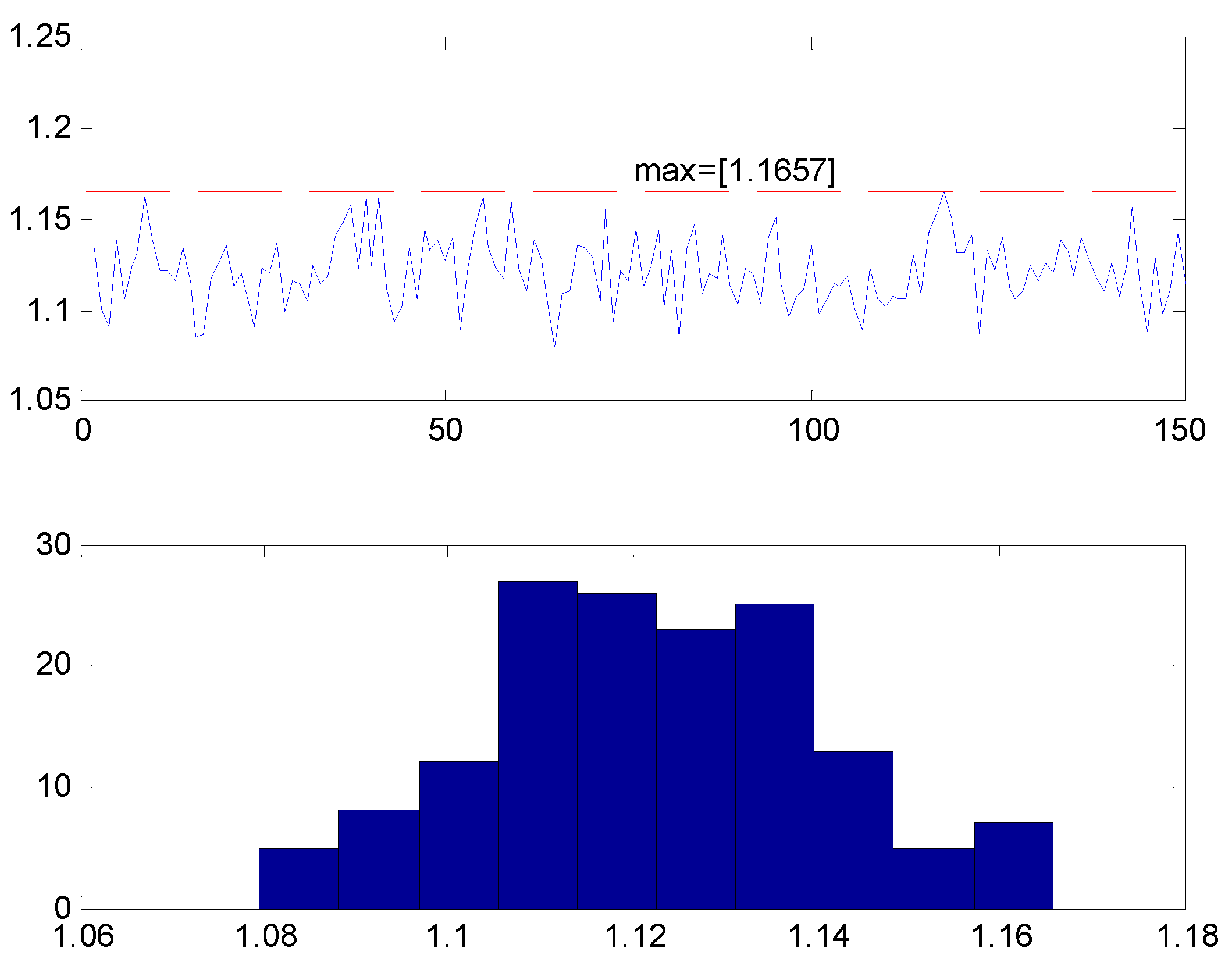
. The bounding factor 1.25, which was obtained heuristically, is a very conservative value. In the following figures, a high number of cases, for high values of n, were processed. In each individual case, a covariance matrix was generated randomly, and its bound was evaluated by an optimization process. All the obtained values were lower than 1.25 (in fact lower than 1.2).

Figure 1. Best evaluated bounds, for 167 cases. For each case, the bound was estimated by binary search. The maximum one was k=1.1714, what is far lower than the proposed k*=1.25.

3.1. What Happens in the Unlikely Cases in Which the Bounding Matrix is Not True?

The probability of that situation happening is very low; but the event is not impossible. However, the question should be asked in terms of risk. The risk is extremely low as well, because even not satisfying the bounding condition, the effect of it is marginal, in similar way as numerical errors in updating covariance matrixes would not affect when those are applied a low frequency. In practical terms the effect of this bounding matrix being overconfident is marginal, in comparison with other sources of inconsistency (numerical, linearization, non-whiteness of noise, etc.). In terms of cost, the cost of applying it is N²; however, it is still remarkably lower than cases in which SVD or other approaches are used. In addition, the scaling is applied in the GCKF context, where global updates are low frequency operations.

3.2. Pathological Cases

Cases in which the covariance matrix has rank=1, may need a more conservative bound. For example, cases in which P = A*A^T, in which A is a rectangular matrix of very few columns. In must be noted that for estimation problems in which the state vector is high dimensional, that situation is extremely unusual, which the exception of highly correlated SLAM (Simultaneous Localization and Mapping) problems. For that reason, we have tested the approach in a highly correlated SLAM case, to verify the approximation process in a demanding case.

4. SLAM Case

The low precision version of the GCKF was applied to the SLAM case, similar to that previously presented in [1], however in this case a mono-agent SLAM has been considered, for a more compact presentation of the results. It can be seen that the discrepancy between the full precision version and the integer versions is marginal, for all the cases.

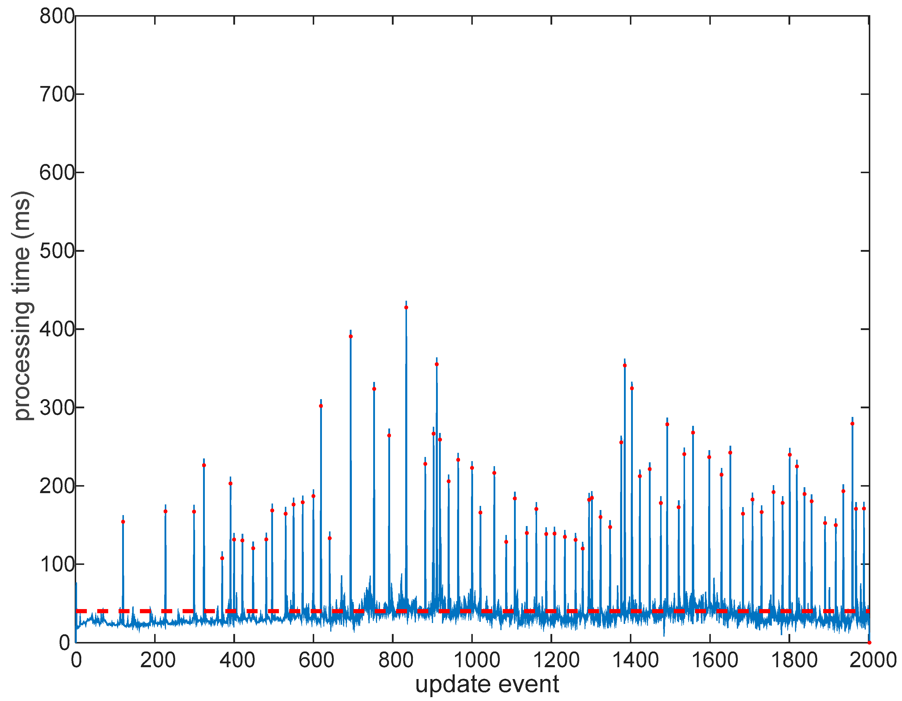
The covariance matrix is offered in blocks, under request from clients (in place of requiring full conversion between integer precision and nominal precision); consequently, there is an improvement in processing time, due to the way the computer memory is used. These improvements are appreciated in the times needed for processing the global updates, as shown in the processing times for the usual GCKF and its version operating in low precision floating point format, in the high dimensional global component of the GCKF. 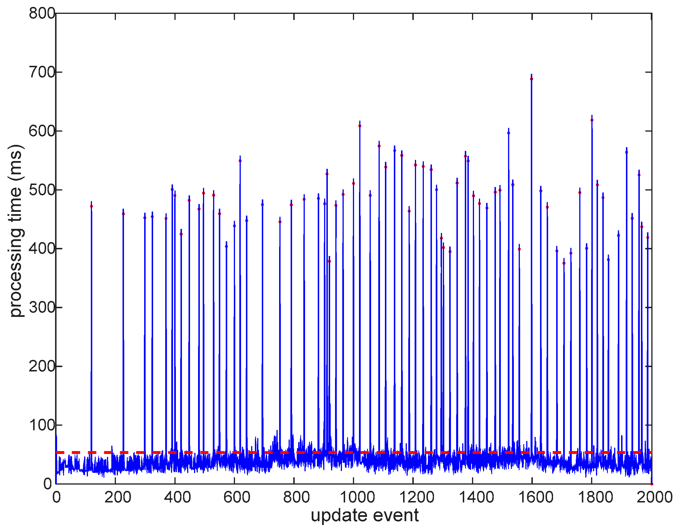The standard version is shown in Figure 2. GCKF operating in double precision (in all its components, global low-frequency and high-frequency subsystems). Update times. When a low-frequency global update is required, the usual peak in the processing time does occur. The average processing time (37ms) is well lower than that of a full filter, but still the peaks may represent an issue in may applications (as those peaks reached up 700ms). GCKF Update events at which a global update was performed are indicated by a red dot in the associated processing time.

4.1. Description of the SLAM Process

The SLAM process is performed in a simulated context of operation, in which the Objects of Interests (OOIs) are detected well spread in the area of operation. In addition to those landmarks, walls are also present, so that occlusions to the sensors’ visibility is also included, for making the simulation realistic.The SLAM process is performed considering that no speed measurements are available, but IMU gyroscope is present (although it is polluted by bias, whose value is also estimated). The observability of the full SLAM process is still achieved due to the high number of landmarks usually detected. Observations are range and bearing; however, the quality of the range components is poor, in comparison to those of bearing. Discrepancies between actual (i.e., simulated) values and the expected values of position, heading and speed and angular velocity are provided. Those always show proper consistency. We focused our attention on the performance of the suboptimal approach being tested, comparing its results to those of the optimal full GCKF.

Update processing times, for the GCKF operating under low precision global PDF. The usual peaks, for those updates which required a global update are well less expensive than those equivalent ones in the full precision standard GCKF. This saving in processing time is achieved at no sacrifice in accuracy. The saving in processing times is mostly due to aspects related to memory usage (e.g., fewer RAM cache misses) than to actual processing effort. It is worth noting that both experiments are identical, even in the instance of noises.

It is interesting to appreciate the processing times at non-GU (global update) times (at which the updates just occur in the high frequency estimation processes, not involving a global update). Those processing times do slowly increase as the estimation keeps progressing during the SLAM process. That increase is due to the increase in number of states, as the map’s size does increase in the exploration. The processing times corresponding to global update events are also affected by the increase in the number of states being estimated, as the map does grow.

Figure 3. GCKF operating in low precision (its global PDF component exploiting the single precision bounding approach). The update processing times, for the GCKF operating under low precision global PDF. The usual peaks, for those updates which required a global update, are well less expensive than those equivalent ones in the full precision standard GCKF. This saving in processing time is achieved at negligible sacrifice in accuracy. The saving in processing times is mostly due to aspects related to memory usage (e.g., fewer RAM cache misses) than to actual processing effort. It is worth noting that both experiments are identical, even the instance of noises. The high-frequency processing components are identical. The only difference is related to the low-frequency global component of the GCKF, which maintain if full covariance matrix in low precision numerical format and bounds it to guarantee estimation consistency.

The average time is 40% lower than that of the full precision mode (35ms against 75ms). However, the relevant benefit is more related to the reduction in the cost of the sporadic global updates of the GCKF, and on saving memory. The usual peaks, for those updates which required a global update are well less expensive than those equivalent ones in the full precision standard GCKF. This saving in processing time is achieved at no sacrifice in accuracy. The saving in processing times is mostly due to aspects related to memory usage (e.g., fewer RAM cache misses) than to actual processing effort. It is worth noting that both experiments are identical, even the instance of noises. A question would be “Where is the saving in processing time?”. A critical component in the answer would be that by reducing the required memory for the large covariance matrix and the frequency at which is fully accessed, the number of cache misses are reduced dramatically, resulting in latencies closer to those of the static RAM of the cache memories. That is an intrinsic benefit of using the GCKF. The proposed new additional processing further improves the efficiency of the GCKF in accessing memory. It can be seen that for the standard GCKF, the peaks of processing time do happen at the times of the global updates. With the additional capability of storing the covariance matrix in low precision numerical format, we are improving it, in average, by a 50% reduction in processing time. Each EKF update usually processed 70 scalar observations (about 35 landmarks being detected / scan. Those were grouped in sets of 15 / updates, requiring multiple individual updates for completing the update. In addition, iterations were applied treating the non-linear observation equations (few iterations, usually 3)

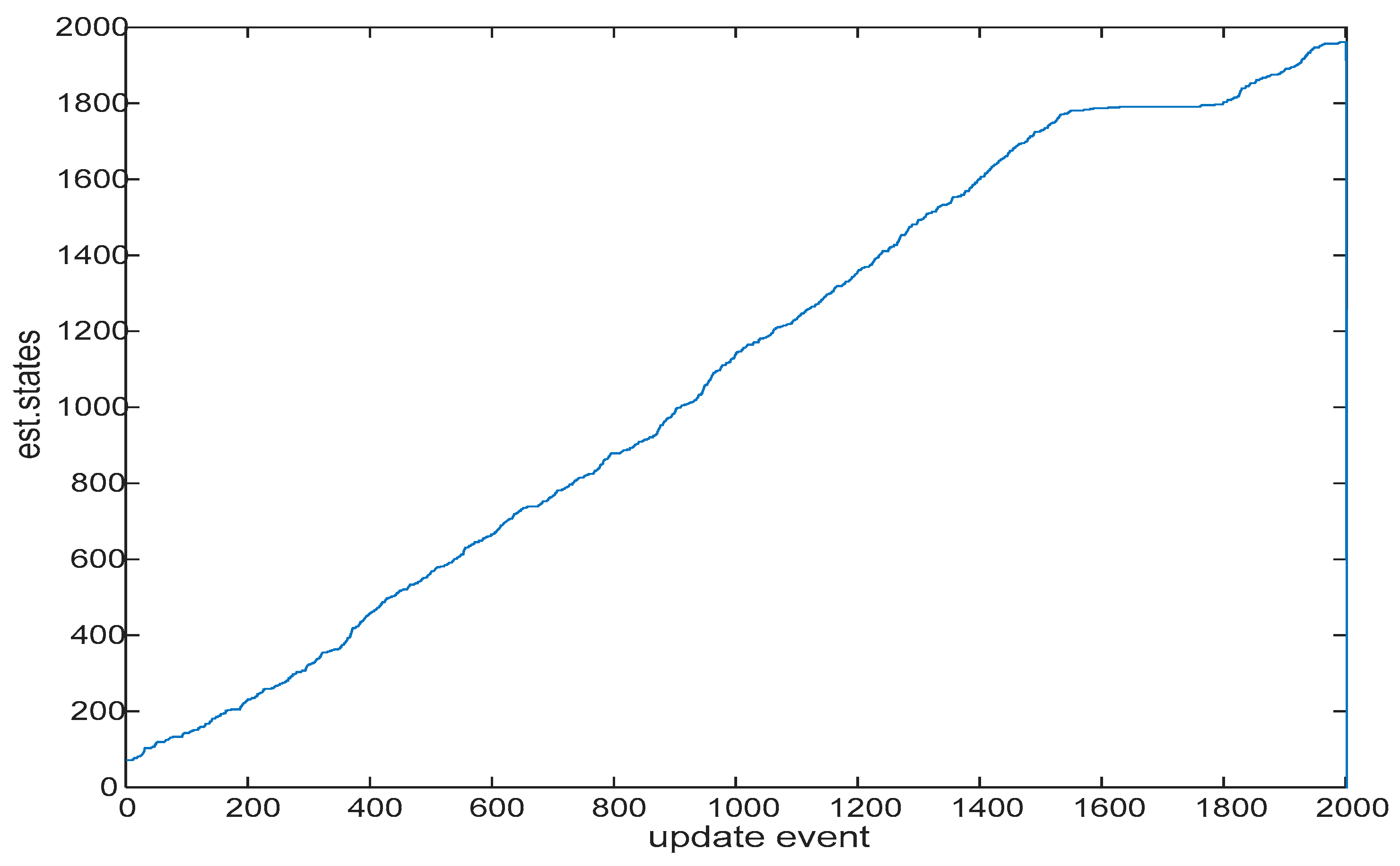
Figure 4. Number of states in the state vector being estimated, growing during the first phase of the SLAM process, when the map is being explored for its first time. In this part of the test, the SLAM process was in its exploration stage, and new areas were seen for their first time, making the state vector to grow in length. The process reached 2 kilo-states,.

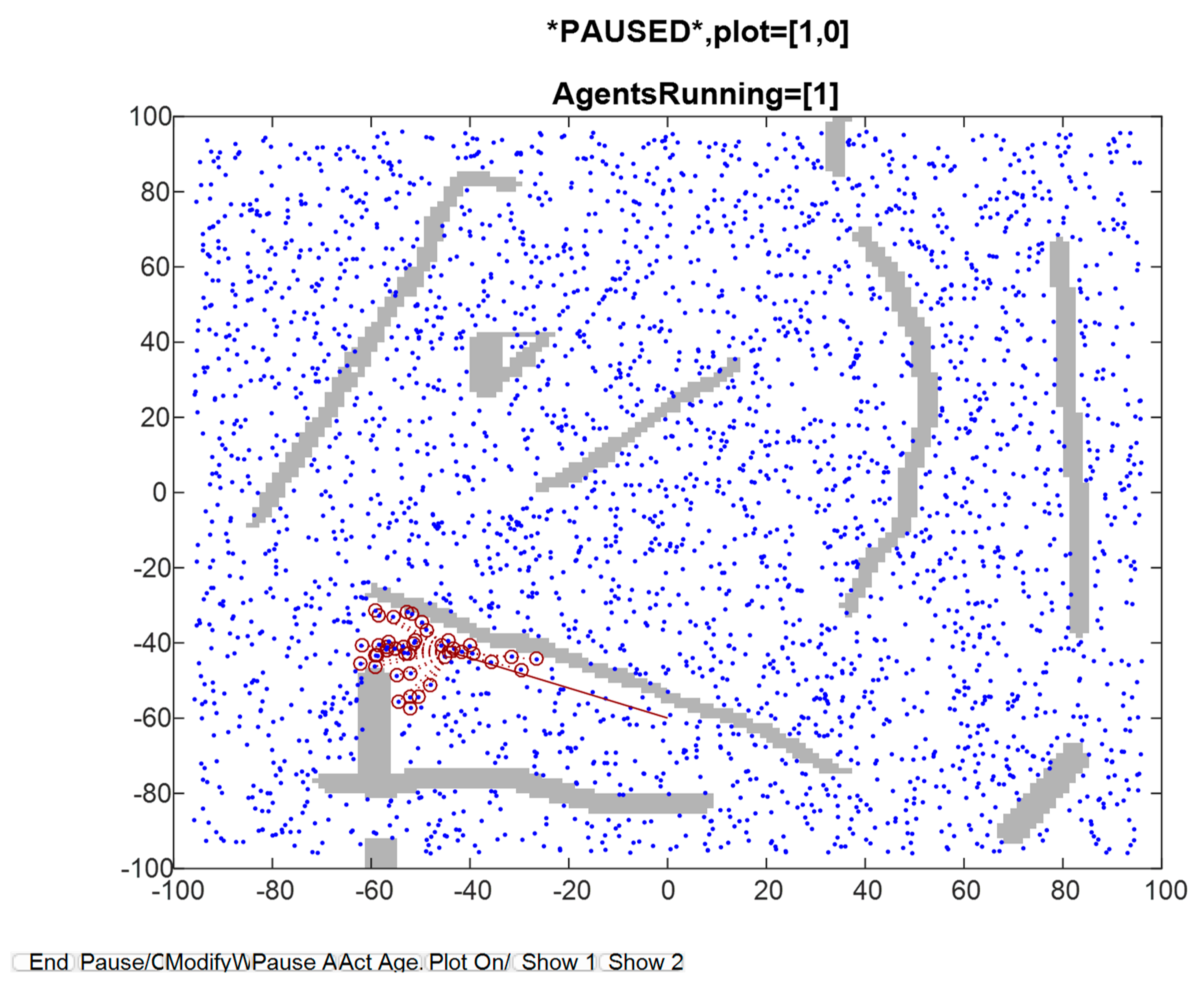
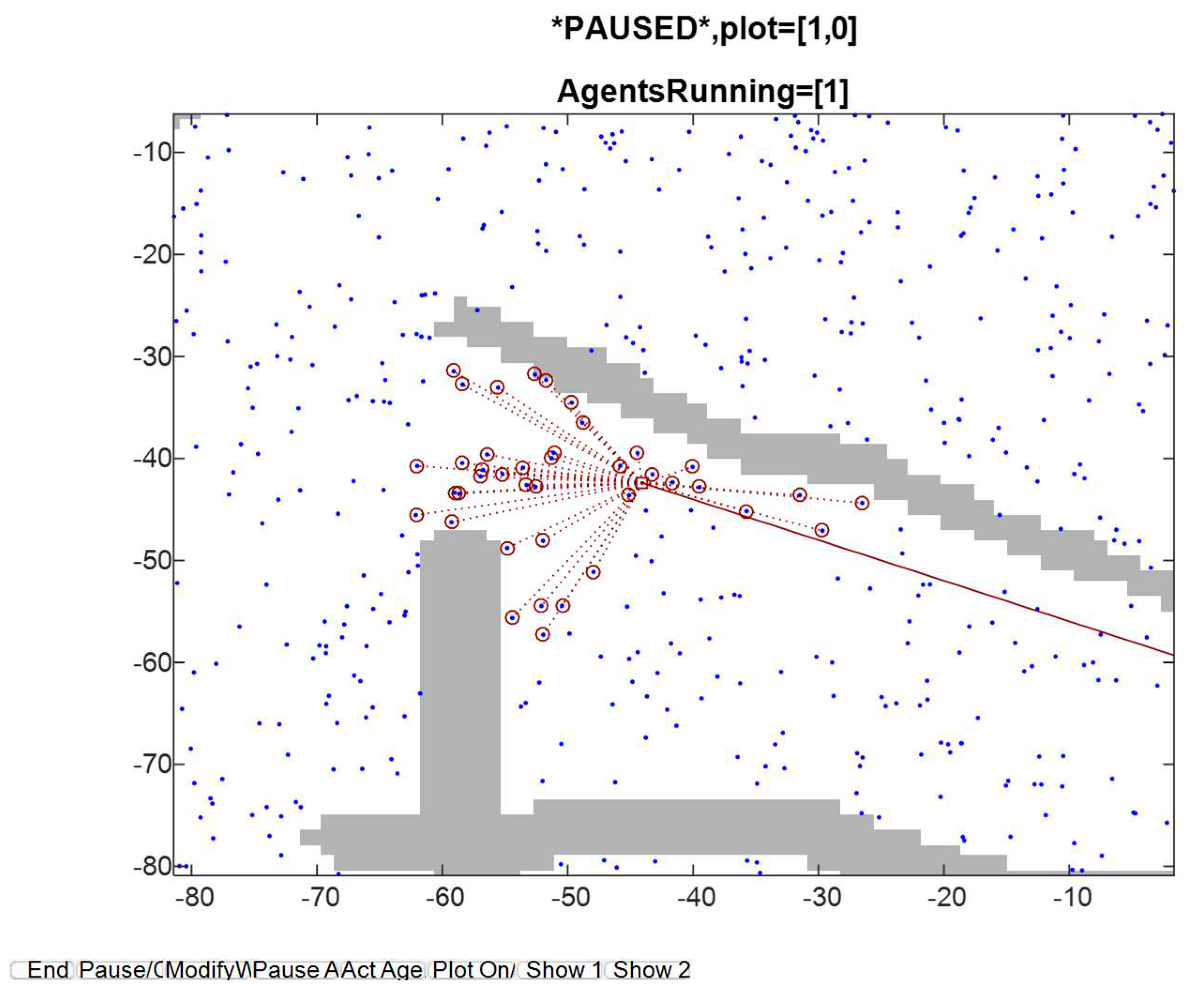
Figure 5. Full view, taken at certain update event. The blue dots are OOIs (Objects of interest) on the terrain, which usually constitute landmarks. The travelled path, until that time, is indicated by a red curve.

Figure 6. An image showing, in more detail, the OOI being detected in the previous figure.

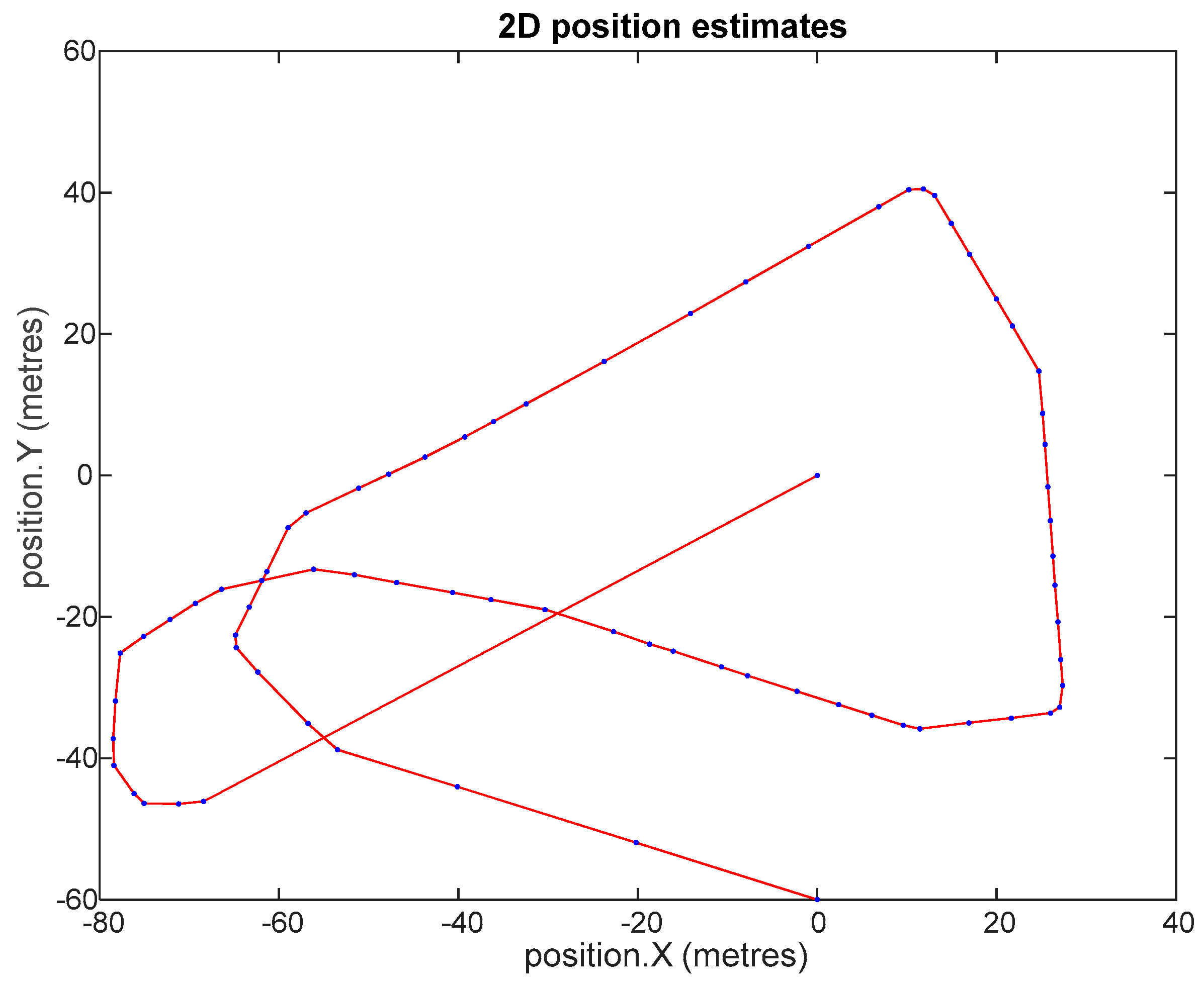
Figure 7. Platform ‘s 2D position estimates, for the GCKF SLAM (double and single precision covariance matrix, and single precision bounded version.). Maximum discrepancy was about 0.3 mm, which is not appreciable due to the scale. Multiple loop closures did happen during the trip.

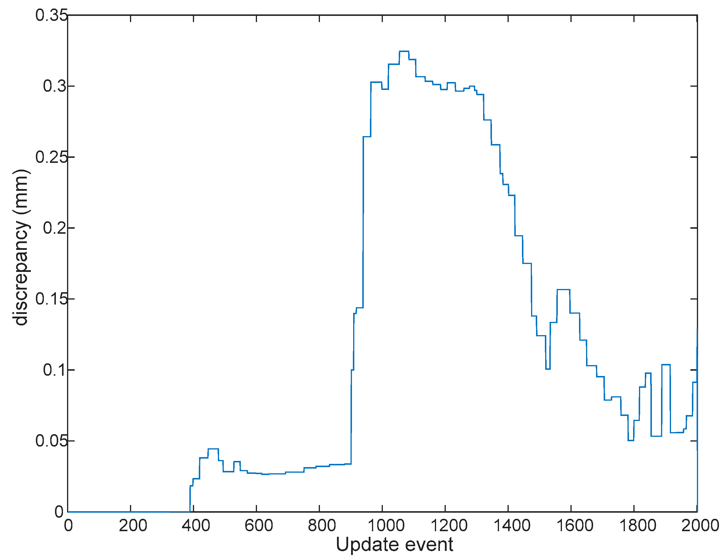
Figure 8. Discrepancy between platform’s 2D position estimates, for the GCKF SLAM (standard double precision covariance matrix, and single precision bounded version.). Maximum discrepancy was about 0.3 mm. There is a peak at the time associated to the update event 1100, and then a decrease in error. It coincides with the first loop closure of the SLAM process, at which the estimates become more accurate and more confident. The values are distances in 2D.

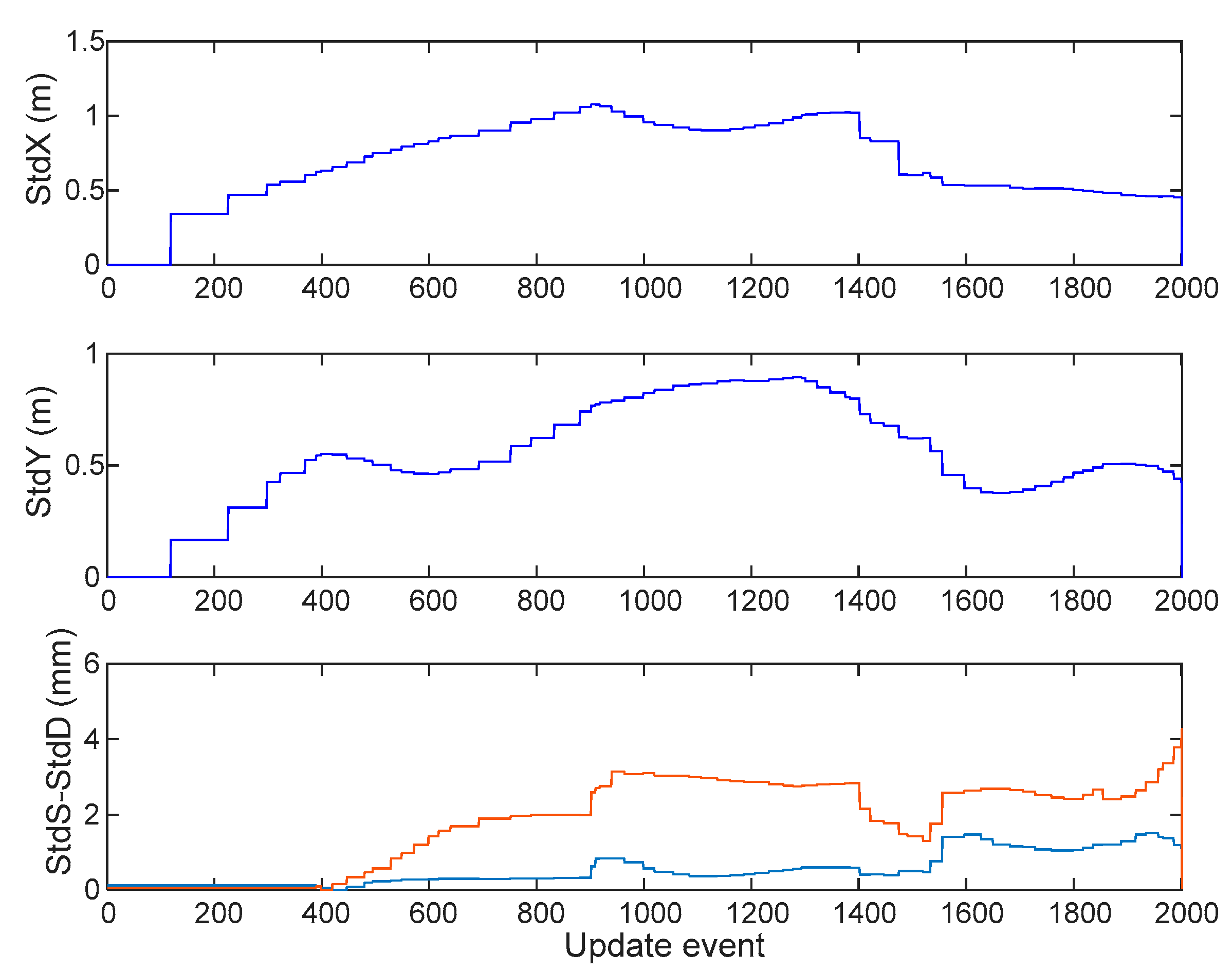
Figure 9. The top two plots show the standard deviations (in meters) of the marginal PDFs of the double precision GCKF process, for the estimates of (x,y) position of the platform, at each time during the trip. The bottom figure shows the differences between those standard deviations (in millimeters) for x and y, between the standard double precision GCKF and those of the single precision one. The one based on the bounded single precision covariance matrix is always slightly more conservative than the standard one. Those values are also consistent with the discrepancies in the expected values. This is a relevant result, as the SLAM process usually implies a cumulative error as the platform travels far away, only to be mitigated by the loop closures.

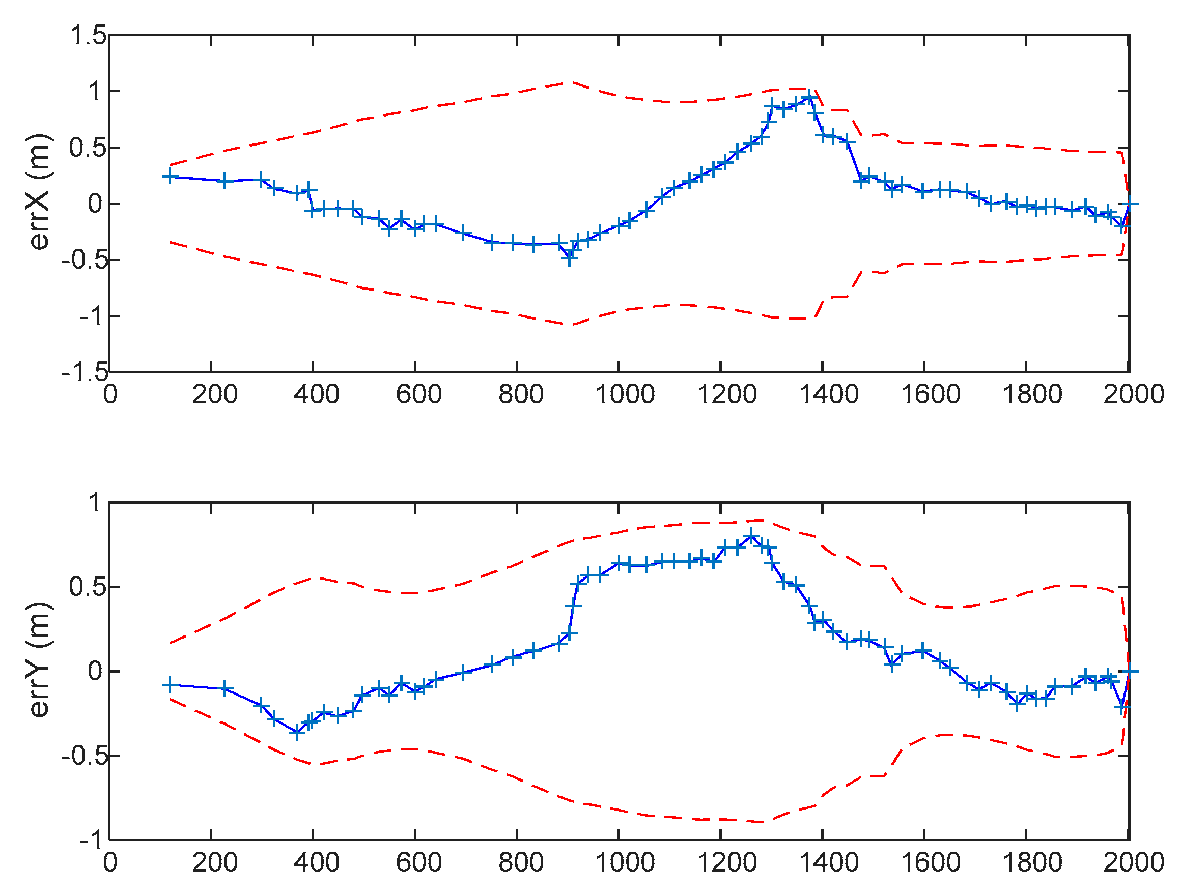
Figure 10. Absolute discrepancy between estimates expected values and ground truth, at those times of the GCKF global updates (blue). The reported standard deviations of the associated 1D marginal PDFs are shown in red broken lines, this is for both, the standard GCKF and the single precision one (as both are almost identical when shown in that scale). As it is usual in SLAM Bayesian processes, the accuracy of the estimates is time varying, particular evident when loop closured do occur, in which the estimates get more confident, as indicated by the decreasing standard deviations of the marginal PDFs.

5. Conclusions and Future Work

The proposed approach for bounding large covariance matrixes by a low precision representation is simple and easy for being applied. It may not be powerful if used at high frequency, however in conjunction in the GCKF framework it is a valuable contribution. The improvement in processing times is adequate for many applications which require real-time performance.

This modification of the GCKF is one of many more being considered by the authors. One of the next objectives is developing an asynchronous version of the GCKF, for spreading the cost of the global updates in time, making the estimation process free of those low frequency but expensive updates. The research also involves the development of a decentralized version able to operate in networked contexts. In all those variants we intend to include, usually required extra processing in the low frequency component of the GCKF, which result in low overall processing cost. Alternative approaches of bounding the full covariance matrix are also being considered. It is of interest for us to consider other strategies for reducing the processing cost related to the global updates of the GCKF, in particular those techniques related dimensionality reduction.

References

Guivant, J.E. The Generalized Compressed Kalman Filter. Robotica 2017, 35, 1639–1669. [Google Scholar] [CrossRef]
Narula, J.E.G.K. Switching and information exchange in compressed estimation of coupled high dimensional processes. Automatica 2019, 99, 149–156. [Google Scholar] [CrossRef]
Narula, J.G.X.L.K. Non-linear Estimation with Generalised Compressed Kalman Filter; International Conference on Information Fusion (FUSION): Cambridge, UK, 2018. [Google Scholar]
Guivant, J.; Nebot, E. Optimization of the simultaneous localization and map-building algorithm for real-time implementation. IEEE Trans. Robot. Autom. 2001, 17, 242–257. [Google Scholar] [CrossRef]
Guivant, J.; Nebot, E. Solving computational and memory requirements of feature-based simultaneous localization and mapping algorithms. IEEE Trans. Robot. Autom. 2003, 19, 749–755. [Google Scholar] [CrossRef]
Cheng, J.; Kim, J. Compressed Unscented Kalman Filter-Based SLAM. in International Conference on Robotics and Biomimetics, USA, 2014.
Guivant, J. Efficient simultaneous localization and mapping in large environments. Ph.D. Thesis, The University of Sydney, Sydney, Australia, 2002. [Google Scholar]
Guivant, J. The Compressed Extended Kalman Filter. 2002. Available online: www.cas.kth.se/SLAM/Presentations/cekf.pdf (accessed on 25 July 2015).
Lin, J.; Xie, L.; Xiao, W. Target tracking in wireless sensor networks using compressed Kalman filter. Int. J. Sens. Networks 2009, 6, 251–262. [Google Scholar] [CrossRef]
Roumeliotis, S.; Burdick, J. Stochastic cloning: a generalized framework for processing relative state measurements. in IEEE International Conference onRobotics and Automation, 2002.
Mourikis, A.I.; Roumeliotis, S.I.; Burdick, J.W. SC-KF Mobile Robot Localization: A Stochastic Cloning Kalman Filter for Processing Relative-State Measurements. IEEE Trans. Robot. 2007, 23, 717–730. [Google Scholar] [CrossRef]
Nebot, E.; Lee, G.K.F.; Brubaker, T.A. Experiments on a single-link flexible manipulator. in USA-Japan Symp. on Flexible Automation, 1988.
Bailey, T.; Durrant-Whyte, H. Simultaneous localization and mapping (SLAM): part II. IEEE Robot. Autom. Mag. 2006, 13, 108–117. [Google Scholar] [CrossRef]
Bailey, T.; Durrant-Whyte, H. Simultaneous localization and mapping (SLAM): part II. IEEE Robot. Autom. Mag. 2006, 13, 108–117. [Google Scholar] [CrossRef]
Barton, M.J.; Robinson, P.A.; Kumar, S.; Galka, A.; Durrant-Whyte, H.F.; Guivant, J.; Ozaki, T. Evaluating the Performance of Kalman-Filter-Based EEG Source Localization. IEEE Trans. Biomed. Eng. 2008, 56, 122–136. [Google Scholar] [CrossRef] [PubMed]
Julier, S. The stability of covariance inflation methods for SLAM. in IEEE International Conference on Intelligent Robots and Systems, 2003.
Lopez, J.D.; Espinosa, J.J. Spatio-temporal EEG brain imaging based on reduced Kalman filtering; IEEE/EMBS International Conference on Neural Engineering (NER): Cancun, Mexico, 2011. [Google Scholar]
Neira, J.; Tardos, J. Data association in stochastic mapping using the joint compatibility test. IEEE Trans. Robot. Autom. 2001, 17, 890–897. [Google Scholar] [CrossRef]
Houtekamer, P.L.; Mitchell, H.L. Ensemble Kalman Filtering. Q.J.R. Meteorol 2006, 131, 3269–3289. [Google Scholar] [CrossRef]
Houtekamer, P.L.; Mitchell, H.L. Data Assimilation Using an Ensemble Kalman Filter Technique. Mon. Weather. Rev. 1998, 126, 796–811. [Google Scholar] [CrossRef]
Evensen, G. The Ensemble Kalman Filter: theoretical formulation and practical implementation. Ocean Dyn. 2003, 53, 343–367. [Google Scholar] [CrossRef]
Paz, L.M.; Tardós, J.D.; Neira, J. ; Divide and Conquer: EKF SLAM in O(n). IEEE Trans. Robot. 2008, 24, 1107–1120. [Google Scholar] [CrossRef]
Knight, J.; Davison, A.; Reid, I. Towards constant time SLAM using postponement. in IEEE/RSJ International Conference on Intelligent Robots and Systems, 2001.
Williams, S. Efficient Solutions to Autonomous Mapping and Navigation Problems; The University of Sydney: Sydney, Australia, 2001. [Google Scholar]
Julier, S.J.; Uhlmann, J.K. Unscented Filtering and Nonlinear Estimation. Proc. IEEE 2004, 92, 401–422. [Google Scholar] [CrossRef]
Cheng, J.; Kim, J.; Shao, J.; Zhang, W. Robust linear pose graph-based SLAM. Robot. Auton. Syst. 2015, 72, 71–82. [Google Scholar] [CrossRef]

Figure 2. GCKF operating in double precision (in all its components, global low-frequency and high-frequency subsystems). Update times. When a low-frequency global update is required, the usual peak in the processing time does occur. The average processing time (37ms) is well lower than of that of a full filter, but still the peaks may represent an issue in may applications (as those peaks reached up to 700ms). GCKF Update events at which a global update was performed are indicated by a red dot in the associated processing time.

Disclaimer/Publisher’s Note: The statements, opinions and data contained in all publications are solely those of the individual author(s) and contributor(s) and not of MDPI and/or the editor(s). MDPI and/or the editor(s) disclaim responsibility for any injury to people or property resulting from any ideas, methods, instructions or products referred to in the content.

© 2023 by the authors. Licensee MDPI, Basel, Switzerland. This article is an open access article distributed under the terms and conditions of the Creative Commons Attribution (CC BY) license (http://creativecommons.org/licenses/by/4.0/).

Copyright: This open access article is published under a Creative Commons CC BY 4.0 license, which permit the free download, distribution, and reuse, provided that the author and preprint are cited in any reuse.