Quick and Complete Convergence in the Law of Large Numbers with Applications to Statistics

1. Introduction

In [1], Hsu and Robbins introduced the notion of complete convergence which is stronger than almost sure (a.s.) convergence. Hsu and Robbins used this notion to discuss certain aspects of the Law of Large Numbers (LLN). In particular, let $X_1,X_2,\cdots$ be independent and identically distributed (i.i.d.) random variables with the common mean $\mu =\mathsf{E}\left[X_1\right]$. Hsu and Robbins proved that, while in the Kolmogorov Strong Law of Large Numbers (SLLN), only the first moment condition is needed for the sample mean $n^{-1}{\sum }_{t=1}^n{X}_t$ to converge to $\mu$ as $n\to \infty$, the complete version of the SLLN requires the second-moment condition $\mathsf{E}|X_1{|}^2<\infty$ (finiteness of variance). Later, Baum and Katz [2], working on the rate of convergence in the LLN, established that the second-moment condition is not only necessary but also sufficient for complete convergence. Strassen [3] introduced another mode of convergence, the r-quick convergence. When $r=1$, these two modes of convergence are closely related. In the case of i.i.d. random variables and the sample mean $n^{-1}{\sum }_{t=1}^n{X}_t$, they are identical. This fact and certain statistical applications motivated Tartakovsky [4] (see also Tartakovsky [5] and Tartakovsky et al. [6]) to introduce a natural generalization of complete convergence – the r-complete convergence, which turns out to be identical to the r-quick convergence in the i.i.d. case.

Section 2 discusses pure probabilistic issues related to r-complete convergence and r-quick convergence. Section 3 explores statistical applications in sequential hypothesis testing and changepoint detection. Section 4 outlines sufficient conditions for r-complete convergence for Markov and hidden Markov models, which is needed to establish optimality properties of sequential hypothesis tests and changepoint detection procedures. Section 5 concludes.

2. Modes of Convergence and the Law of Large Numbers

We begin by listing some standard definitions in probability theory. Let $(\Omega ,\mathcal{F})$ be a measurable space, i.e., $\Omega$ is a set of elementary events $\omega$ and $\mathcal{F}$ is a sigma-algebra (a system of subsets of $\Omega$ satisfying standard conditions). A probability space is a triple $(\Omega ,\mathcal{F},\mathsf{P})$, where $\mathsf{P}$ is a probability measure (completely additive measure normalized to 1) defined on the sets from the sigma-algebra $\mathcal{F}$. More specifically, by Kolmogorov’s axioms, probability $\mathsf{P}$ satisfies: $\mathsf{P}\left(\mathcal{A}\right)\ge 0$ for any $\mathcal{A}\in \mathcal{F}$; $\mathsf{P}(\Omega )=1$; and $\mathsf{P}\left({\cup }_{i=1}^{\infty }{\mathcal{A}}_i\right)={\sum }_{i=1}^{\infty }\mathsf{P}\left({\mathcal{A}}_i\right)$ for ${\mathcal{A}}_i\in \mathcal{F}$, ${\mathcal{A}}_i\cap {\mathcal{A}}_j=⌀$, $i\ne j$, where ⌀ is an empty set.

A function $X=X\left(\omega \right)$ defined on $(\Omega ,\mathcal{F})$ with values in $\mathcal{X}$ is called random variable if it is $\mathcal{F}$-measurable, i.e., $\{\omega :X(\omega )\in B\}$ belongs to the sigma-algebra $\mathcal{F}$. The function $F\left(x\right)=\mathsf{P}(\omega :X(\omega )\le x)$ is the distribution function of X. It is also referred to as cumulative distribution function (cdf). The real-valued random variables $X_1,X_2,\cdots$ are independent if the events $\{X_1\le x_1\},\{X_2\le x_2\},\cdots$ are independent for every sequence $x_1,x_2,\cdots$ of real numbers. In what follows, we shall deal with real-valued random variables unless specified otherwise.

2.1. Standard Modes of Convergence

Let X be a random variable and let ${\left\{X_n\right\}}_{n\in {\mathbb{Z}}_{+}}$ (${\mathbb{Z}}_{+}=\{0,1,2,\cdots \}$) be a sequence of random variables, both defined on the probability space $(\Omega ,\mathcal{F},\mathsf{P})$. We now give several standard definitions and results related to the Law of Large Numbers.

Convergence in Distribution (Weak Convergence). Let $F_n\left(x\right)=\mathsf{P}(\omega :X_n\le x)$ be the cdf of $X_n$ and let $F\left(x\right)=\mathsf{P}(\omega :X\le x)$ be the cdf of X. We say that the sequence ${\left\{X_n\right\}}_{n\in {\mathbb{Z}}_{+}}$ converges to X in distribution (or in law or weakly) as $n\to \infty$ and write $X_n\underset{n\to \infty }{\overset{\mathrm{law}}{\to }}X$ if

$$\underset{n\to \infty }{lim}{F}_n\left(x\right)=F\left(x\right)$$

at all continuity points of $F\left(x\right)$.

Convergence in Probability. We say that the sequence ${\left\{X_n\right\}}_{n\in {\mathbb{Z}}_{+}}$ converges to X in probability as $n\to \infty$ and write $X_n\underset{n\to \infty }{\overset{\mathsf{P}}{\to }}X$ if

$$\underset{n\to \infty }{lim}\mathsf{P}\left(\right|X_n-X|>\epsilon )=0\mathrm{for}\mathrm{every}\epsilon >0.$$

Almost Sure Convergence. We say that the sequence ${\left\{X_n\right\}}_{n\in {\mathbb{Z}}_{+}}$ converges to X almost surely (a.s.) or with probability 1 (w.p. 1) as $n\to \infty$ under probability measure $\mathsf{P}$ and write $X_n\underset{n\to \infty }{\overset{\mathsf{P}-\mathrm{a}.\mathrm{s}.}{\to }}X$ if

$$\mathsf{P}\left(\omega :\underset{n\to \infty }{lim}{X}_n=X\right)=1.$$

(1)

It is easily seen that (1) is equivalent to the condition

$$\underset{n\to \infty }{lim}\mathsf{P}\left(\omega :\sum _{t=n}^{\infty }|X_t-X|>\epsilon \right)=0\mathrm{for}\mathrm{every}\epsilon >0,$$

and that the a.s. convergence implies convergence in probability, and the convergence in probability implies convergence in distribution, while the converse statements are not generally true.

The following double implications that establish necessary and sufficient conditions (i.e., equivalences) for the a.s. convergence are useful:

$$X_n\underset{n\to \infty }{\overset{\mathrm{a}.\mathrm{s}.}{\to }}X⟺\mathsf{P}\left(\underset{t\ge n}{sup}|X_t-X|>\epsilon \right)\underset{n\to \infty }{\to }0\mathrm{for}\mathrm{all}\epsilon >0.$$

(2)

The following result is often useful.

Lemma 1.

Let $f\left(t\right)$ be a nonnegative increasing function, ${lim}_{t\to \infty }f\left(t\right)=\infty$. If

$$\frac{X_n}{f\left(n\right)}\underset{n\to \infty }{\overset{\mathsf{P}-\mathrm{a}.\mathrm{s}.}{\to }}0,$$

then

$$\underset{n\to \infty }{lim}\mathsf{P}\left(\frac{1}{f\left(n\right)}\underset{0\le t\le n}{max}{X}_t>\epsilon \right)=0\mathit{for}\mathit{every}\epsilon >0.$$

(3)

Proof. 

For any $\epsilon >0$, $n_0>0$ and $n>n_0$, we have

$$\begin{array}{cc}\hfill \mathsf{P}\left(\frac{1}{f\left(n\right)}\underset{0\le t\le n}{max}{X}_t>\epsilon \right)& \le \mathsf{P}\left(\frac{1}{f\left(n\right)}\underset{0\le t\le n_0}{max}{X}_t>\epsilon \right)+\mathsf{P}\left(\frac{1}{f\left(n\right)}\underset{n_0<t\le n}{max}{X}_t>\epsilon \right)\hfill \\ \hfill & \le \mathsf{P}\left(\frac{1}{f\left(n\right)}\underset{0\le t\le n_0}{max}{X}_t>\epsilon \right)+\mathsf{P}\left(\underset{t>n_0}{max}\frac{X_t}{f\left(t\right)}>\epsilon \right).\hfill \end{array}$$

Letting $n\to \infty$ and taking into account that

$$\underset{n\to \infty }{lim}\mathsf{P}\left(\frac{1}{f\left(n\right)}\underset{0\le t\le n_0}{max}{X}_t>\epsilon \right)=0,$$

we obtain

$$\begin{array}{cc}\hfill \underset{n\to \infty }{lim\; sup}\mathsf{P}\left(\frac{1}{f\left(n\right)}\underset{0\le t\le n}{max}{X}_t>\epsilon \right)& \le \mathsf{P}\left(\underset{t>n_0}{sup}\frac{X_t}{f\left(t\right)}>\epsilon \right).\hfill \end{array}$$

Since $n_0$ can be arbitrarily large, we can let $n_0\to \infty$ and since, by assumption $X_n/f\left(n\right)\underset{n\to \infty }{\overset{\mathrm{a}.\mathrm{s}.}{\to }}0$, it follows from (2) that the upper bound approaches 0 as $n_0\to \infty$. This completes the proof. □

Remark 1.

The proof of Lemma 1 shows that the assertion (3) also holds under the one-sided condition

$$\mathsf{P}\left(\underset{t>n}{sup}\frac{X_t}{f\left(t\right)}>\epsilon \right)\underset{n\to \infty }{\to }0\mathit{for}\mathit{all}\epsilon >0.$$

(4)

Random Walk. Let $X_0,X_1,X_2,\cdots$ be i.i.d. random variables with mean $\mathsf{E}\left[X_n\right]=\mu$ for $n\ge 1$ and the initial condition $X_0=x$. Then $S_n={\sum }_{t=0}^n{X}_t$ is called a random walk with mean $x+\mu n$.

In what follows, in the case where $X_1,X_2,\cdots$ are i.i.d. random variables and $S_n={\sum }_{t=0}^n{X}_t$, we prefer to formulate the results in terms of the random walk ${\left\{S_n\right\}}_{n\in {\mathbb{Z}}_{+}}$ (typically $S_0=0$ while not necessarily).

We now recall the two Strong Law of Large Numbers (SLLN). Write $S_n=X_0+X_1+\cdots +X_n$ for the partial sum ($X_0=S_0=0$), so that ${\left\{S_n\right\}}_{n\in {\mathbb{Z}}_{+}}$ is a random walk with zero initial condition as long as $X_1,X_2,\cdots$ are i.i.d. with mean $\mu$.

Kolmogorov’s SLLN. Let ${\left\{S_n\right\}}_{n\in {\mathbb{Z}}_{+}}$ be a random walk under probability measure $\mathsf{P}$. If $\mathsf{E}\left[S_1\right]$ exists, then the sample mean $S_n/n$ converges to the mean value $\mathsf{E}\left[S_1\right]$ w.p. 1, i.e.,

$$n^{-1}{S}_n\underset{n\to \infty }{\overset{\mathsf{P}-\mathrm{a}.\mathrm{s}.}{\to }}\mathsf{E}\left[S_1\right].$$

(5)

Conversely, if $n^{-1}{S}_n\underset{n\to \infty }{\overset{\mathsf{P}-\mathrm{a}.\mathrm{s}.}{\to }}\mu$, where $\left|\mu \right|<\infty$, then $\mathsf{E}\left[S_1\right]=\mu$.

Marcinkiewicz-Zygmund’s SLLN. Let ${\left\{S_n\right\}}_{n\in {\mathbb{Z}}_{+}}$ be a zero-mean random walk under probability measure $\mathsf{P}$. The following two statements are equivalent:

(i) $\mathsf{E}|S_1{|}^p<\infty$ for $0<p<2$;

(ii) $n^{-1/p}{S}_n\underset{n\to \infty }{\overset{\mathsf{P}-\mathrm{a}.\mathrm{s}.}{\to }}0$.

2.2. Complete and r-Complete Convergence

We begin with discussing the issue of rates of convergence in the LLN.

Rates of Convergence. Let ${\left\{X_n\right\}}_{n\in {\mathbb{Z}}_{+}}$ be a sequence of random variables and assume that $X_n$ converges to 0 w.p. 1 as $n\to \infty$. The question is what the rate of convergence is? In other words, how fast does the tail probability $\mathsf{P}\left(\right|X_n|>\epsilon )$ decay to zero? This question can be answered by analyzing the behavior of the sums

$$\Sigma (r,\epsilon ):=\sum _{n=1}^{\infty }{n}^{r-1}\mathsf{P}\left(\right|X_n|>\epsilon )\mathrm{for}\mathrm{some}r>0\mathrm{and}\mathrm{all}\epsilon >0.$$

More specifically, if $\Sigma (r,\epsilon )$ is finite for every $\epsilon >0$, then the tail probability $\mathsf{P}\left(\right|X_n|>\epsilon )$ decays with the rate faster than $1/n^r$, so that $n^r\mathsf{P}\left(\right|X_n|>\epsilon )\to 0$ for all $\epsilon >0$ as $n\to \infty$.

To answer these questions we now consider modes of convergence that strengthen the almost sure convergence, and therefore, help to determine the rate of convergence in the SLLN. Historically this issue was first addressed in 1947 by Hsu and Robbins [1] who introduced the new mode of convergence that they called Complete Convergence.

Complete Convergence. The sequence ${\left\{X_n\right\}}_{n\in {\mathbb{Z}}_{+}}$ converges to 0 completely if

$$\underset{n\to \infty }{lim}\sum _{i=n}^{\infty }\mathsf{P}\left(\right|X_t|>\epsilon )=0\mathrm{for}\mathrm{every}\epsilon >0.$$

(6)

Clearly, (6) is equivalent to

$$\Sigma (1,\epsilon )=\sum _{n=1}^{\infty }\mathsf{P}\left(\right|X_n|>\epsilon )<\infty \mathrm{for}\mathrm{every}\epsilon >0.$$

Also, (6) implies a.s. convergence $X_n\underset{n\to \infty }{\overset{\mathrm{a}.\mathrm{s}.}{\to }}0$, but converse is not generally true unless the variables $X_1,X_2,\cdots$ are not independent.

Let ${\left\{S_n\right\}}_{n\in {\mathbb{Z}}_{+}}$ be a random walk with mean $\mathsf{E}\left[S_n\right]=\mu n$. Kolmogorov’s SLLN (5) implies that the sample mean $S_n/n$ converges to $\mu$ w.p. 1. Hsu and Robbins [1] proved that under the same assumptions (i.e., under the only first-moment condition $\mathsf{E}|S_1|<\infty$) the sequence ${\left\{n^{-1}{S}_n\right\}}_{n\ge 1}$ need not converge to $\mu$ completely, but it will do so under the further second-moment condition $\mathsf{E}|S_1{|}^2<\infty$. So the finiteness of variance is a sufficient condition for complete convergence in the SLLN. They conjectured that the second-moment condition is not only sufficient but also necessary for complete convergence. Thus, it follows from these results that if the variance is finite, then the rate of convergence in Kolmogorov’s SLLN is ${lim}_{n\to \infty }n\mathsf{P}\left(\right|S_n/n-\mu |>\epsilon )=0$ for all $\epsilon >0$.

A further step towards this issue was done in 1965 by Baum and Katz [2]. In particular, the following result follows from Theorem 3 in [2] for the random walk ${\left\{S_n\right\}}_{n\in {\mathbb{Z}}_{+}}$ with mean $\mathsf{E}\left[S_1\right]=\mu$.

Theorem 1.

Let $r>0$ and $\alpha >1/2$. If ${\left\{S_n\right\}}_{n\in {\mathbb{Z}}_{+}}$ is a random walk with mean $\mathsf{E}\left[S_1\right]=\mu$, then the following statements are equivalent:

$$\begin{array}{cc}\hfill \mathsf{E}\left[\right|S_1{|}^{(r+1)/\alpha }]<\infty & ⟺\sum _{n=1}^{\infty }{n}^{r-1}\mathsf{P}\left\{\frac{1}{n^{\alpha }}|S_n-\mu n|>\epsilon \right\}<\infty \mathit{for}\mathit{all}\epsilon >0\hfill \\ \hfill & ⟺\sum _{n=1}^{\infty }{n}^{r-1}\mathsf{P}\left\{\underset{k\ge n}{sup}\frac{1}{k^{\alpha }}|S_k-\mu k|>\epsilon \right\}<\infty \mathit{for}\mathit{all}\epsilon >0.\hfill \end{array}$$

(7)

Setting $r=1$ and $\alpha =1$ in (7), we obtain the following equivalence

$$\mathsf{E}\left[\right|S_1{|}^2]<\infty ⟺\sum _{n=1}^{\infty }\mathsf{P}\left\{|S_n/n-\mu |>\epsilon \right\}\mathrm{for}\mathrm{all}\epsilon >0,$$

which shows that the conjecture of Hsu and Robbins is correct – the second-moment condition $\mathsf{E}|S_1{|}^2<\infty$ is both necessary and sufficient for complete convergence

$$n^{-1}{S}_n\underset{n\to \infty }{\overset{\mathsf{P}-\mathrm{completely}}{\to }}\mu .$$

Furthermore, if for some $r>0$ the $(r+1)$-th moment is finite, $\mathsf{E}|S_1{|}^{r+1}<\infty$, then the rate of convergence in the SLLN is ${lim}_{n\to \infty }{n}^r\mathsf{P}\left(\right|S_n/n-\mu |>\epsilon )=0$ for all $\epsilon >0$.

Previous results suggest that it is reasonable to generalize the notion of complete convergence into the following mode of convergence that we will refer to as r-Complete Convergence, which is also related to the so-called r-Quick Convergence that we will discuss later on (see Subsection 2.3).

Definition 1

(r-Complete Convergence). Let $r>0$. We say that the sequence of random variables ${\left\{X_n\right\}}_{n\in {\mathbb{Z}}_{+}}$ converges to X r-completelyas $n\to \infty$ under probability measure $\mathsf{P}$ and write $X_n\underset{n\to \infty }{\overset{\mathsf{P}\text{-}r\text{-}\mathrm{completely}}{\to }}X$ if

$$\Sigma (r,\epsilon ):=\sum _{n=1}^{\infty }{n}^{r-1}\mathsf{P}\left(\right|X_n-X|>\epsilon )<\infty \mathit{for}\mathit{every}\epsilon >0.$$

(8)

Note that the a.s. convergence of $\left\{X_n\right\}$ to X can be equivalently written as

$$\underset{n\to \infty }{lim}\mathsf{P}\left(\sum _{i=n}^{\infty }|X_t-X|>\epsilon \right)=0\mathrm{for}\mathrm{every}\epsilon >0,$$

so that the r-complete convergence with $r\ge 1$ implies the a.s. convergence, but the converse is not true in general.

Suppose that $X_n$ converges a.s. to X. If $\Sigma (r,\epsilon )$ is finite for every $\epsilon >0$, then

$$\underset{n\to \infty }{lim}\sum _{t=n}^{\infty }{t}^{r-1}\mathsf{P}\left(\right|X_t-X|>\epsilon )=0\mathrm{for}\mathrm{every}\epsilon >0$$

and probability $\mathsf{P}\left(\right|X_n-X|>\epsilon )$ goes to 0 as $n\to \infty$ with the rate faster than $1/n^r$. Hence, as already mentioned above, the r-complete convergence allows one to determine the rate of convergence of $X_n$ to X, i.e., to answer the question on how fast the tail probability $\mathsf{P}\left(\right|X_n-X|>\epsilon )$ decays to zero.

The following result provides a very useful implication of complete convergence.

Theorem 2.

Let ${\left\{X_n\right\}}_{n\in {\mathbb{Z}}_{+}}$ and ${\left\{Y_n\right\}}_{n\in {\mathbb{Z}}_{+}}$ be two arbitrary, possibly dependent sequences of random variables. Assume that there are positive and finite numbers ${\mu }_1$ and ${\mu }_2$ such that

$$\sum _{n=1}^{\infty }\mathsf{P}\left(|\frac{1}{n}{X}_n-{\mu }_1|>\epsilon \right)<\infty \mathit{for}\mathit{every}\epsilon >0$$

(9)

and

$$\sum _{n=1}^{\infty }\mathsf{P}\left(|\frac{1}{n}{Y}_n-{\mu }_2|>\epsilon \right)<\infty \mathit{for}\mathit{every}\epsilon >0,$$

(10)

i.e., $n^{-1}{X}_n\underset{n\to \infty }{\overset{\mathsf{P}-\mathrm{completely}}{\to }}{\mu }_1$ and $n^{-1}{Y}_n\underset{n\to \infty }{\overset{\mathsf{P}-\mathrm{completely}}{\to }}{\mu }_2$. If ${\mu }_1\ge {\mu }_2$, then for any random time T

$$\mathsf{P}\left(X_T<b,Y_{T+1}\ge b(1+\delta )\right)⟶0\mathit{as}b\to \infty \mathit{for}\mathit{any}\delta >0.$$

(11)

Proof. 

Fix $\delta >0$, $c\in (0,\delta )$ and let $N_b=⌈1+c)b/{\mu }_2⌉$ be the smallest integer that is larger than or equal to $(1+c)b/{\mu }_2$. Observe that

$$\begin{array}{cc}\hfill \mathsf{P}\left(X_T<b,Y_{T+1}\ge b(1+\delta )\right)& \le \mathsf{P}\left(X_T\le b,T\ge N_b\right)+\mathsf{P}\left(Y_{T+1}\ge (1+\delta )b,T<N_b\right)\hfill \\ \hfill & \le \mathsf{P}\left(X_T\le b,T\ge N_b\right)+\mathsf{P}\left(\underset{1\le n\le N_b}{max}{Y}_n\ge (1+\delta )b\right).\hfill \end{array}$$

Thus, to prove (11) it suffices to show that the two terms on the right-hand side go to 0 as $b\to \infty$.

For the first term, we notice that for any $n\ge N_b$,

$$\frac{b}{n}\le \frac{b}{N_b}\le \frac{{\mu }_2}{1+c}\le \frac{{\mu }_1}{1+c}<{\mu }_1,$$

so that

$$\begin{array}{cc}\hfill \mathsf{P}\left(X_T\le b,T\ge N_b\right)& =\sum _{n=N_b}^{\infty }\mathsf{P}\left(X_n\le b,T=n\right)\le \sum _{n=N_b}^{\infty }\mathsf{P}\left(\frac{X_n}{n}\le \frac{b}{n}\right)\hfill \\ \hfill & \le \sum _{n=N_b}^{\infty }\mathsf{P}\left(\frac{X_n}{n}\le \frac{{\mu }_1}{1+c}\right)=\sum _{n=N_b}^{\infty }\mathsf{P}\left(\frac{X_n}{n}-{\mu }_1\le -\frac{c}{1+c}{\mu }_1\right).\hfill \end{array}$$

Since $N_b\to \infty$ as $b\to \infty$ the upper bound goes to 0 as $b\to \infty$ due to condition (9).

Next, since $c\in (0,\delta )$ there exists ${\epsilon }^{\prime }>0$ such that

$$\frac{(1+\delta )b}{N_b}=\frac{(1+\delta )b}{⌈b(1+c)/{\mu }_2⌉}\ge (1+{\epsilon }^{\prime }){\mu }_2.$$

As a result,

$$\begin{array}{c}\hfill \mathsf{P}\left(\underset{1\le n\le N_b}{max}{Y}_n\ge (1+\delta )b\right)\le \mathsf{P}\left(\frac{1}{N_b}\underset{1\le n\le N_b}{max}{Y}_n\ge (1+{ϵ}^{\prime }){\mu }_2\right),\end{array}$$

where the upper bound goes to 0 as $b\to \infty$ by condition (10) (see Lemma 1). □

Remark 2.

The proof suggests that the assertion (11) of Theorem 2 holds under the following one-sided conditions

$$\begin{array}{c}\hfill \mathsf{P}\left(n^{-1}\underset{1\le s\le n}{max}{Y}_s-{\mu }_2>\epsilon \right)\underset{n\to \infty }{\to }0,\sum _{n=1}^{\infty }\mathsf{P}\left(n^{-1}{X}_n-{\mu }_1<-\epsilon \right)<\infty .\end{array}$$

Complete convergence conditions (9) and (10) guarantee both these conditions.

Remark 3.

Theorem 2 can be applied to the overshoot problem. Indeed, if $X_n=Y_n=Z_n$ and the random time T is the first time n when $Z_n$ exceeds the level b, $T=inf\{n\ge 1:Z_n>b\}$, then Theorem 2 shows that the relative excess of boundary crossing (overshoot) $(Z_T-b)/b$ converges to 0 in probability as $b\to \infty$ when $Z_n/n$ converges completely as $n\to \infty$ to a positive number μ.

2.3. r-Quick Convergence

In 1967, Strassen [3] introduced the notion of r-quick limit points of a sequence of random variables. The r-quick convergence has been further addressed by Lai [7,8], Chow and Lai [9], Fuh and Zhang [10], and Tartakovsky [4,5] (see certain details in Subsection 2.4).

We define r-quick convergence in a way suitable for this paper. Let ${\left\{X_n\right\}}_{n\in {\mathbb{Z}}_{+}}$ be a sequence of real-valued random variables and let X be a random variable defined on the same probability space $(\Omega ,\mathcal{F},\mathsf{P})$.

Definition 2

(r-Quick Convergence). Let $r>0$ and for $\epsilon >0$ let

$$L_{\epsilon }=sup\{n\ge 1:|X_n-X|>\epsilon \}(sup\{⌀\}=0)$$

be the last entry time of $X_n$ in the region $(X+\epsilon ,\infty )\cup (-\infty ,X-\epsilon )$. We say that the sequence ${\left\{X_n\right\}}_{n\in {\mathbb{Z}}_{+}}$ converges to X r-quickly as $n\to \infty$ under probability measure $\mathsf{P}$ and write $X_n\underset{n\to \infty }{\overset{\mathsf{P}-r\text{-}\mathrm{quickly}}{\to }}X$ if, and only if,

$$\mathsf{E}\left[L_{\epsilon }^r\right]<\infty \mathit{for}\mathit{every}\epsilon >0,$$

(12)

where $\mathsf{E}$ is the operator of expectation under probability $\mathsf{P}$.

This definition can be of course generalized to random variables X, ${\left\{X_n\right\}}_{n\in {\mathbb{Z}}_{+}}$ taking values in a metric space $(\mathcal{X},d)$ with distance d: $X_n\underset{n\to \infty }{\overset{r\text{-}\mathrm{quickly}}{\to }}X$ if

$$\mathsf{E}\left[{\left(sup\{n\ge 1:d(X,X_n)>\epsilon \}\right)}^r\right]<\infty \mathrm{for}\mathrm{every}\epsilon >0.$$

Note that the a.s. convergence $X_n\to \mu$ ($\left|\mu \right|<\infty$) as $n\to \infty$ to a constant $\mu$ can be expressed as $\mathsf{P}(L_{\epsilon }\left(\mu \right)<\infty )=1$, where $L_{\epsilon }\left(\mu \right)=sup\{n\ge 1:|X_n-\mu |>\epsilon \}$ . Therefore, the r-quick convergence implies the convergence w.p. 1 but not conversely.

Note also that in general r-quick convergence is stronger than r-complete convergence. Specifically, the following lemma shows that

$$\underset{1\le i\le n}{max}{X}_t\underset{n\to \infty }{\overset{r-\mathrm{completely}}{\to }}\mu ⟹X_n\underset{n\to \infty }{\overset{r-\mathrm{quickly}}{\to }}\mu ⟹X_n\underset{n\to \infty }{\overset{r-\mathrm{completely}}{\to }}\mu .$$

(13)

Lemma 2.

Let ${\left\{X_n\right\}}_{n\in {\mathbb{Z}}_{+}}$ be a sequence of random variables. Let $f\left(t\right)$ be a nonnegative increasing function, $f\left(0\right)=0$, ${lim}_{t\to \infty }f\left(t\right)=+\infty$, and let for $\epsilon >0$

$$L_{\epsilon }\left(f\right)=sup\left\{n\ge 1:|X_n|>\epsilon f\left(n\right)\right\}(sup\{⌀\}=0)$$

be the last time $X_n$ leaves the interval $[-\epsilon f(n),+\epsilon f(n\left)\right]$.

(i) For any $r>0$ and any $\epsilon >0$ the following inequalities hold:

$$\begin{array}{c}\hfill r\sum _{n=1}^{\infty }{n}^{r-1}\mathsf{P}\left\{|X_n|\ge \epsilon f\left(n\right)\right\}\le \mathsf{E}\left[L_{\epsilon }{\left(f\right)}^r\right]\le r\sum _{n=1}^{\infty }{n}^{r-1}\mathsf{P}\left\{\underset{t\ge n}{sup}\frac{|X_t|}{f\left(t\right)}\ge \epsilon \right\}.\end{array}$$

(14)

Therefore,

$$\sum _{n=1}^{\infty }{n}^{r-1}\mathsf{P}\left\{\underset{t\ge n}{sup}\frac{|X_t|}{f\left(t\right)}\ge \epsilon \right\}<\infty \mathit{for}\mathit{all}\epsilon >0⟹X_n\underset{n\to \infty }{\overset{r\text{-}\mathrm{quickly}}{\to }}0.$$

(ii) If $f\left(t\right)$ is a power function, $f\left(t\right)=t^{\gamma }$, $\gamma >0$, then finiteness of

$$\sum _{n=1}^{\infty }{n}^{r-1}\mathsf{P}\left\{\underset{1\le t\le n}{max}{X}_t\ge \epsilon n^{\gamma }\right\}$$

for some $r>0$ and every $\epsilon >0$ implies r-quick convergence of $X_n$ to 0:

$$\left\{\sum _{n=1}^{\infty }{n}^{r-1}\mathsf{P}\left(\underset{1\le t\le n}{max}{X}_t\ge \epsilon n^{\gamma }\right)<\infty \forall \epsilon >0\right\}⟹\left\{\mathsf{E}\left[L_{\epsilon }{\left(\gamma \right)}^r\right]<\infty \forall \epsilon >0\right\},$$

(15)

where $L_{\epsilon }\left(\gamma \right)=sup\left\{n\ge 1:|X_n|>\epsilon n^{\gamma }\right\}$.

Proof. 

(i) Obviously,

$$\mathsf{P}\left\{|X_n|\ge \epsilon f\left(n\right)\right\}\le \mathsf{P}\left\{L_{\epsilon }\left(f\right)\ge n\right\}\le \mathsf{P}\left\{\underset{t\ge n}{sup}\frac{1}{f\left(t\right)}\left|X_t\right|\ge \epsilon \right\}$$

from which the inequalities (14) follow immediately.

(ii) Write $M_u={max}_{1\le n\le \lceil u\rceil }\left|X_n\right|$, where $\lceil u\rceil$ is an integer part of u. We have the following chain of inequalities and equalities:

$$\begin{array}{cc}\hfill & \mathsf{E}\left[L_{2\epsilon }{\left(\gamma \right)}^r\right]\le r{\int }_0^{\infty }{t}^{r-1}\mathsf{P}\left\{\underset{u\ge t}{sup}{u}^{-\gamma }\left|X_u\right|\ge 2\epsilon \right\}\mathrm{d}t\hfill \\ \hfill & \le r{\int }_0^{\infty }{t}^{r-1}\mathsf{P}\left\{\underset{u\ge t}{sup}\left[|X_u|-\epsilon u^{\gamma }\right]\ge \epsilon t^{\gamma }\right\}\mathrm{d}t\hfill \\ \hfill & \le r{\int }_0^{\infty }{t}^{r-1}\mathsf{P}\left\{\underset{u>0}{sup}\left[|X_u|-\epsilon u^{\gamma }\right]\ge \epsilon t^{\gamma }\right\}\mathrm{d}t\hfill \\ \hfill & \le r\sum _{n=1}^{\infty }{\int }_0^{\infty }{t}^{r-1}\mathsf{P}\left\{\underset{(2^{n-1}-1)t^{\gamma }<u^{\gamma }\le (2^n-1)t^{\gamma }}{sup}\left[|X_u|-\epsilon u^{\gamma }\right]\ge \epsilon t^{\gamma }\right\}\mathrm{d}t\hfill \\ \hfill & \le r\sum _{n=1}^{\infty }{\int }_0^{\infty }{t}^{r-1}\mathsf{P}\left\{\underset{u^{\gamma }\le 2^n{t}^{\gamma }}{sup}\left|X_u\right|\ge 2^{n-1}\epsilon t^{\gamma }\right\}\mathrm{d}t\hfill \\ \hfill & =r\sum _{n=1}^{\infty }{\int }_0^{\infty }{t}^{r-1}\mathsf{P}\left\{M_{2^{n/\gamma }u}\ge 2^{n-1}\epsilon t^{\gamma }\right\}\mathrm{d}t\hfill \\ \hfill & =r\left[\sum _{n=1}^{\infty }{2}^{-n/\gamma }\right]{\int }_0^{\infty }{u}^{r-1}\mathsf{P}\left\{M_u\ge (\epsilon /2)u^{\gamma }\right\}\mathrm{d}u.\hfill \end{array}$$

It follows that

$$\begin{array}{cc}\hfill & \mathsf{E}\left[L_{2\epsilon }{\left(\gamma \right)}^r\right]\le r{\left(2^{1/\gamma }-1\right)}^{-1}{\int }_0^{\infty }{u}^{r-1}\mathsf{P}\left\{M_u\ge (\epsilon /2)u^{\gamma }\right\}\mathrm{d}u\le \hfill \end{array}$$

(16)

$$\begin{array}{cc}\hfill & \le r{\left(2^{1/\gamma }-1\right)}^{-1}\sum _{n=1}^{\infty }{n}^{r-1}\mathsf{P}\left\{\underset{1\le t\le n}{max}{X}_n\ge \epsilon n^{\gamma }\right\}\hfill \end{array}$$

(17)

which yields the implication (15) and completes the proof. □

The following theorem shows that, in the i.i.d. case, the implications in (13) become equivalences.

Theorem 3.

Let ${\left\{S_n\right\}}_{n\in {\mathbb{Z}}_{+}}$ be the random walk with mean $\mathsf{E}\left[S_n\right]=\mu n$. The following statements are equivalent

$$\begin{array}{cc}\hfill \mathsf{E}|S_1{|}^{r+1}<\infty & ⟺n^{-1}{S}_n\underset{n\to \infty }{\overset{r-\mathrm{completely}}{\to }}\mu ,\hfill \end{array}$$

(18)

$$\begin{array}{cc}\hfill \mathsf{E}|S_1{|}^{r+1}<\infty & ⟺n^{-1}{S}_n\underset{n\to \infty }{\overset{r-\mathrm{quickly}}{\to }}\mu ,\hfill \end{array}$$

(19)

$$\begin{array}{cc}\hfill \mathsf{E}|S_1{|}^{r+1}& ⟺\sum _{n=1}^{\infty }{n}^{r-1}\mathsf{P}\left\{\underset{k\ge n}{sup}\frac{1}{k}\left|S_k-\mu \right|>\epsilon \right\}<\infty \mathit{for}\mathit{all}\epsilon >0.\hfill \end{array}$$

(20)

Proof. 

By Theorem 1, in the i.i.d. case,

$$\begin{array}{c}\hfill \mathsf{E}|S_1{|}^{r+1}<\infty ⟺\sum _{n=1}^{\infty }{n}^{r-1}\mathsf{P}\left(\frac{1}{n}\left|S_n-\mu \right|>\epsilon \right)<\infty \forall \epsilon >0\end{array}$$

(21)

and

$$\mathsf{E}|S_1{|}^{r+1}<\infty ⟺\sum _{n=1}^{\infty }{n}^{r-1}\mathsf{P}\left(\underset{k\ge n}{sup}\frac{1}{k}\left|S_k-\mu \right|>\epsilon \right)<\infty \forall \epsilon >0,$$

(22)

so that assertion (18) follows from (21) and (20) from (22).

Next, let

$$L_{\epsilon }=sup\left\{n\ge 1:|S_n-n\mu |\ge n\epsilon \right\}(sup⌀=0).$$

By Lemma 2(i),

$$\mathsf{E}\left[L_{\epsilon }^r\right]\le r\sum _{n=1}^{\infty }{n}^{r-1}\mathsf{P}\left\{\underset{t\ge n}{sup}\left(|S_t-\mu t|/t\right)\ge \epsilon \right\}\forall \epsilon >0,$$

(23)

which along with (22) implies (19).

2.4. Further Remarks on r-Complete Convergence, r-Quick Convergence and Rates of Convergence in SLLN

Let ${\left\{S_n\right\}}_{n\in {\mathbb{Z}}_{+}}$ be a random walk. Without loss of generality let $S_0=0$ and $\mathsf{E}\left[S_1\right]=0$.

1. Strassen [3] proved, in particular, that if $f\left(n\right)={(2nlogn)}^{1/2}$ in Lemma 2, then for $r>0$

$$\underset{n\to \infty }{lim\; sup}\frac{S_n}{\sqrt{2nlogn}}=\sqrt{r\mathsf{E}\left[S_1^2\right]}r-\mathrm{quickly}$$

(24)

whenever $\mathsf{E}|S_1{|}^p<\infty$ for $p>(2r+1)$. He also proved the functional form of the law of the iterated logarithm.

2. Lai [7] improved this result showing that Strassen’s moment condition $\mathsf{E}|S_1{|}^p<\infty$ for $p>(2r+1)$ can be relaxed. Specifically, he showed that a weaker condition

$$\mathsf{E}\left[|S_1{|}^{2(r+1)}({log}^{+}|S_1{|+1)}^{-(r+1)})\right]<\infty \mathrm{for}r>0$$

(25)

is the best one can do (i.e., both necessary and sufficient):

$$\mathsf{E}\left[|S_1{|}^{2(r+1)}({log}^{+}|S_1{|+1)}^{-(r+1)}\right]<\infty ⟺\underset{n\to \infty }{lim\; sup}\frac{S_n}{\sqrt{2nlogn}}<\infty r-\mathrm{quickly},$$

in which case equality (24) holds.

Note, however, that for $r=0$ in terms of the a.s. convergence

$$\mathsf{E}\left[|S_1{|}^2\right]<\infty ⟺\underset{n\to \infty }{lim\; sup}\frac{S_n}{\sqrt{2nloglogn}}=\sqrt{\mathsf{E}\left[|S_1{|}^2\right]}\mathrm{a}.\mathrm{s}.$$

but under condition (25) for all $r>0$

$$\underset{n\to \infty }{lim\; sup}\frac{S_n}{\sqrt{2nloglogn}}=\infty r-\mathrm{quickly}.$$

3. Let $\alpha >1/2$ and $r>0$. Chow and Lai [9] established the following one-sided inequality for tail probabilities:

$$\sum _{n=1}^{\infty }{n}^{r-1}\mathsf{P}\left(\underset{1\le t\le n}{max}{S}_t\ge n^{\alpha }\right)\le C_{r,\alpha }\left\{\mathsf{E}\left[{\left(S_1^{+}\right)}^{(r+1)/\alpha }\right]+{\left(\mathsf{E}\left[S_1^2\right]\right)}^{r/(2\alpha -1)}\right\}$$

(26)

whenever $\mathsf{E}|S_1{|}^2<\infty$. Under the same hypotheses, this one-sided inequality implies the two-sided one:

$$\sum _{n=1}^{\infty }{n}^{r-1}\mathsf{P}\left(\underset{1\le t\le n}{max}\left|S_t\right|\ge n^{\alpha }\right)\le C_{r,\alpha }\left\{\mathsf{E}\left[|S_1{|}^{(r+1)/\alpha }\right]+{\left(\mathsf{E}\left[S_1^2\right]\right)}^{r/(2\alpha -1)}\right\}.$$

(27)

The upper bound in (27) turns out to be sharp since the lower bound also holds:

$$\sum _{n=1}^{\infty }{n}^{r-1}\mathsf{P}\left(\underset{1\le t\le n}{max}\left|S_t\right|\ge n^{\alpha }\right)\ge 1+B_{r,\alpha }\left\{\mathsf{E}\left[|S_1{|}^{(r+1)/\alpha }\right]+{\left(\mathsf{E}\left[S_1^2\right]\right)}^{r/(2\alpha -1)}\right\}.$$

Here the constants $C_{r,\alpha }$ and $B_{r,\alpha }$ are universal depending only on $r,\alpha$.

The results of Chow and Lai [9] provide one-sided analogues of the results of Baum and Katz [2] as well as extend their results. Indeed, the one-sided inequality (26) implies that the following statements are equivalent for the zero-mean random walk:

(i) $\mathsf{E}\left[{\left(S_1^{+}\right)}^{(r+1)/\alpha }\right]<\infty$;

(ii) ${\sum }_{n=1}^{\infty }{n}^{r-1}\mathsf{P}\left(n^{-\alpha }{S}_n\ge \epsilon \right)<\infty \mathrm{for}\mathrm{all}\epsilon >0$;

(iii) ${\sum }_{n=1}^{\infty }{n}^{r-1}\mathsf{P}\left({sup}_{k\ge n}{k}^{-\alpha }{S}_k\ge \epsilon \right)<\infty \mathrm{for}\mathrm{all}\epsilon >0$, where $\alpha >1/2$.

Clearly, the two-sided inequality (27) yields the assertions of Theorem 1 if $\mu =0$.

4. The Marcinkiewicz-Zygmund SLLN states that for $\alpha >1/2$ the following implications hold:

$$\mathsf{E}|S_1{|}^{1/\alpha }<\infty ⟺n^{-\alpha }{S}_n\underset{n\to \infty }{\overset{\mathrm{a}.\mathrm{s}.}{\to }}0.$$

(28)

The strengthened r-quick equivalent of this SLLN is: For any $r>0$ and $\alpha >1/2$ the following statements are equivalent,

$$\begin{array}{cc}\hfill \mathsf{E}\left[\right|S_1{|}^{(r+1)/\alpha }]<\infty & ⟺\sum _{i=1}^{\infty }{n}^{r-1}\mathsf{P}\left\{\frac{1}{n^{\alpha }}\left|S_n\right|>\epsilon \right\}<\infty \mathrm{for}\mathrm{all}\epsilon >0\hfill \\ \hfill & ⟺\sum _{n=1}^{\infty }{n}^{r-1}\mathsf{P}\left\{\underset{k\ge n}{sup}\frac{1}{k^{\alpha }}\left|S_k\right|>\epsilon \right\}<\infty \mathrm{for}\mathrm{all}\epsilon >0\hfill \\ \hfill & ⟺n^{-\alpha }{S}_n\underset{n\to \infty }{\overset{r-\mathrm{quickly}}{\to }}0.\hfill \end{array}$$

(29)

Implications (29) follow from Theorem 1, Theorem 3 and inequality (27). The proof is almost obvious and omitted.

3. Applications of r-Complete and r-Quick Convergences in Statistics

In this section, we outline certain statistical applications which show the usefulness of r-complete and r-quick versions of the SLLN.

3.1. Sequential Hypothesis Testing

We begin with formulating the following multihypothesis testing problem for a general non-i.i.d stochastic model. Let $(\Omega ,\mathcal{F},{\mathcal{F}}_n,\mathsf{P})$, $n\in {\mathbb{Z}}_{+}=\{0,1,2,\dots \}$, be a filtered probability space with standard assumptions about the monotonicity of the sub-$\sigma$-algebras ${\mathcal{F}}_n$. The sub-$\sigma$-algebra ${\mathcal{F}}_n=\sigma \left({\mathbf{X}}^n\right)$ of $\mathcal{F}$ is assumed to be generated by the sequence ${\mathbf{X}}^n=\{X_t,1\le t\le n\}$ observed up to time n, which is defined on the space $(\Omega ,\mathcal{F})$. The hypotheses are ${\mathsf{H}}_i:\mathsf{P}={\mathsf{P}}_i$, $i=0,1,\cdots ,N$, where ${\mathsf{P}}_0,{\mathsf{P}}_1,\cdots ,{\mathsf{P}}_N$ are given probability measures assumed to be locally mutually absolutely continuous, i.e., their restrictions ${\mathsf{P}}_i^{\left\{n\right\}}$ and ${\mathsf{P}}_j^{\left\{n\right\}}$ to ${\mathcal{F}}_n$ are equivalent for all $1\le n<\infty$ and all $i,j=0,1,\cdots ,N$, $i\ne j$. Let ${\mathsf{Q}}^{\left\{n\right\}}$ be a restriction to ${\mathcal{F}}_n$ of a $\sigma$-finite measure Q on $(\Omega ,\mathcal{F})$. Under ${\mathsf{P}}_i$ the sample ${\mathbf{X}}^n=(X_1,\cdots ,X_n)$ has a joint density $p_{i,n}\left({\mathbf{X}}^n\right)$ with respect to the dominating measure ${\mathsf{Q}}^{\left(n\right)}$ for all $n\in {\mathbb{Z}}_{+}$, which can be written as

$$p_{i,n}\left({\mathbf{X}}^n\right)=\prod _{t=1}^n{f}_{i,t}\left(X_t\right|{\mathbf{X}}^{t-1}),$$

(30)

where $f_{i,n}\left(X_n\right|{\mathbf{X}}^{n-1})$, $n\ge 1$ are corresponding conditional densities.

Define the likelihood ratio (LR) process between the hypotheses ${\mathsf{H}}_i$ and ${\mathsf{H}}_j$

$${\Lambda }_{ij}\left(n\right)=\frac{\mathrm{d}{\mathsf{P}}_i^{\left\{n\right\}}}{\mathrm{d}{\mathsf{P}}_j^{\left\{n\right\}}}\left({\mathbf{X}}^n\right)=\frac{p_{i,n}\left({\mathbf{X}}^n\right)}{p_{j,n}\left({\mathbf{X}}^n\right)}=\prod _{t=1}^n\frac{f_{i,t}\left(X_t\right|{\mathbf{X}}^{t-1})}{f_{j,t}\left(X_t\right|{\mathbf{X}}^{t-1})}$$

and the log-likelihood ratio (LLR) process

$${\lambda }_{ij}\left(n\right)=log{\Lambda }_{ij}\left(n\right)=\sum _{t=1}^{n}log\left[\frac{f_{i,t}\left(X_t\right|{\mathbf{X}}^{t-1})}{f_{j,t}\left(X_t\right|{\mathbf{X}}^{t-1})}\right],$$

where we set ${\Lambda }_{ij}\left(0\right)=1$ and ${\lambda }_{ij}\left(0\right)=0$.

A multihypothesis sequential test is a pair $\delta =(d,T)$, where T is a stopping time with respect to the filtration ${\left\{{\mathcal{F}}_n\right\}}_{n\in {\mathbb{Z}}_{+}}$ and $d=d\left({\mathbf{X}}^T\right)$ is an ${\mathcal{F}}_T$-measurable terminal decision function with values in the set $\{0,1,\cdots ,N\}$. Specifically, $d=i$ means that the hypothesis ${\mathsf{H}}_i$ is accepted upon stopping, i.e., $\left\{d=i\right\}=\left\{T<\infty ,\delta \mathrm{accepts}{\mathsf{H}}_i\right\}$. Let ${\alpha }_{ij}\left(\delta \right)={\mathsf{P}}_i(d=j)$, $i\ne j$, $i,j=0,1,\cdots ,N$, denote the error probabilities of the test $\delta$, i.e., the probabilities of accepting the hypothesis ${\mathsf{H}}_j$ when ${\mathsf{H}}_i$ is true.

Introduce the class of tests with probabilities of errors ${\alpha }_{ij}\left(\delta \right)$ that do not exceed the prespecified numbers $0<{\alpha }_{ij}<1$:

$$\mathbb{C}\left(\mathbf{\alpha }\right)=\left\{\delta :{\alpha }_{ij}\left(\delta \right)\le {\alpha }_{ij}\mathrm{for}i,j=0,1,\cdots ,N,i\ne j\right\},$$

(31)

where $\mathbf{\alpha }=\left({\alpha }_{ij}\right)$ is a matrix of given error probabilities that are positive numbers less than 1.

Let ${\mathsf{E}}_i$ denote the expectation under the hypothesis ${\mathsf{H}}_i$ (i.e., under the measure ${\mathsf{P}}_i$). The goal of a statistician is to find a sequential test that would minimize the expected sample sizes ${\mathsf{E}}_i\left[T\right]$ for all hypotheses ${\mathsf{H}}_i$, $i=0,1,\cdots ,N$ at least approximately, say asymptotically for small probabilities of errors, i.e., as ${\alpha }_{ij}\to 0$.

3.1.1. Asymptotic Optimality of Walds’s SPRT

Assume first that $N=1$, i.e., that we are dealing with two hypotheses ${\mathsf{H}}_0$ and ${\mathsf{H}}_1$. In the mid 1940s, Wald [11,12] introduced the Sequential Probability Ratio Test (SPRT) for the sequence of i.i.d. observations $X_1,X_2,\cdots$, in which case $f_{i,t}\left(X_t\right|{\mathbf{X}}^{t-1})=f_i\left(X_t\right)$ in (30) and the LR ${\Lambda }_{1,0}\left(n\right)={\Lambda }_n$ is

$${\Lambda }_n=\prod _{t=1}^n\frac{f_1\left(X_t\right)}{f_0\left(X_t\right)}.$$

After n observations have been made Wald’s SPRT prescribes for each $n\ge 1$:

$$\begin{array}{cc}\hfill \mathrm{Stop}\mathrm{and}\mathrm{accept}{H}_1& \mathrm{if}{\Lambda }_n\ge A_1.\hfill \\ \hfill \mathrm{Stop}\mathrm{and}\mathrm{accept}{H}_0& \mathrm{if}{\Lambda }_n\le A_0.\hfill \\ \hfill \mathrm{Continue}\mathrm{sampling}& \mathrm{if}{A}_0<{\Lambda }_n<A_1.\hfill \end{array}$$

where $A_0<1<A_1$ are two thresholds.

Let $Z_t=log[f_1\left(X_t\right)/f_0\left(X_t\right)]$ be the LLR for the observation $X_t$, so the LLR for the sample ${\mathbf{X}}^n$ is the sum

$${\lambda }_{10}\left(n\right)={\lambda }_n=\sum _{t=1}^n{Z}_t,n=1,2,\cdots$$

Let $a_0=-log{A}_0<0$ and $a_1=log{A}_1>0$. The SPRT ${\delta }_{*}(a_0,a_1)=(d_{*},T_{*})$ can be represented in the form

$$T_{*}(a_0,a_1)=inf\left\{n\ge 1:{\lambda }_n\notin (-a_0,a_1)\right\},d_{*}(a_0,a_1)=\left\{\begin{array}{cc}1\hfill & \mathrm{if}{\lambda }_{T_{*}}\ge a_1\hfill \\ 0\hfill & \mathrm{if}{\lambda }_{T_{*}}\le -a_0.\hfill \end{array}\right.$$

(32)

In the case of two hypotheses, the class of tests (31) is of the form

$$\mathbb{C}({\alpha }_0,{\alpha }_1)=\left\{\delta :{\alpha }_0\left(\delta \right)\le {\alpha }_0\mathrm{and}{\alpha }_1\left(\delta \right)\le {\alpha }_1\right\},$$

i.e., it upper-bounds the probabilities of errors of Type 1 (false positive) ${\alpha }_0\left(\delta \right)={\alpha }_{0,1}\left(\delta \right)$ and Type 2 (false negative) ${\alpha }_1\left(\delta \right)={\alpha }_{1,0}\left(\delta \right)$, respectively.

Wald’s SPRT has an extraordinary optimality property: it minimizes both expected sample sizes ${\mathsf{E}}_0\left[T\right]$ and ${\mathsf{E}}_1\left[T\right]$ in the class of sequential (and non-sequential) tests $\mathbb{C}({\alpha }_0,{\alpha }_1)$ with given error probabilities as long as the observations are i.i.d. under both hypotheses. More specifically, Wald and Wolfowitz [13] proved, using a Bayesian approach, that if ${\alpha }_0+{\alpha }_1<1$ and thresholds $-a_0$ and $a_1$ can be selected in such a way that ${\alpha }_0\left({\delta }_{*}\right)={\alpha }_0$ and ${\alpha }_1\left({\delta }_{*}\right)={\alpha }_1$, then the SPRT ${\delta }_{*}$ is strictly optimal in class $\mathbb{C}({\alpha }_0,{\alpha }_1)$. A rigorous proof of this fundamental result is tedious and involves several delicate technical details. Alternative proofs can be found in [14,15,16,17,18,19].

Regardless of the strict optimality of SPRT which holds if, and only if, thresholds are selected so that the probabilities of errors of SPRT are exactly equal to the prescribed values ${\alpha }_0,{\alpha }_1$, which is usually impossible, suppose that thresholds $a_0$ and $a_1$ are so selected that

$$a_0\sim log(1/{\alpha }_1)\mathrm{and}{a}_1\sim log(1/{\alpha }_0)\mathrm{as}{\alpha }_{\max }\to 0.$$

(33)

Then

$${\mathsf{E}}_1\left[T_{*}\right]\sim \frac{|log{\alpha }_0|}{I_1},{\mathsf{E}}_0\left[T_{*}\right]\sim \frac{|log{\alpha }_1|}{I_0}\mathrm{as}{\alpha }_{\max }\to 0,$$

(34)

where $I_1={\mathsf{E}}_1\left[Z_1\right]$ and $I_0={\mathsf{E}}_0[-Z_1]$ are Kullback-Leibler (K-L) information numbers so that the following asymptotic lower bounds for ESS are attained by SPRT:

$$\underset{\delta \in \mathbb{C}({\alpha }_0,{\alpha }_1)}{inf}{\mathsf{E}}_1\left[T\right]\ge \frac{|log{\alpha }_0|}{I_1}+o\left(1\right),\underset{\delta \in \mathbb{C}({\alpha }_0,{\alpha }_1)}{inf}{\mathsf{E}}_0\left[T\right]\ge \frac{|log{\alpha }_1|}{I_0}+o\left(1\right)\mathrm{as}{\alpha }_{\max }\to 0$$

(cf. [6]). Hereafter ${\alpha }_{\max }=max({\alpha }_0,{\alpha }_1)$. The following inequalities for the error probabilities of the SPRT hold in the most general non-i.i.d. case

$${\alpha }_1\left({\delta }_{*}\right)\le exp\{-a_0\}[1-{\alpha }_0\left({\delta }_{*}\right)],{\alpha }_0\left({\delta }_{*}\right)\le exp\{-a_1\}[1-{\alpha }_1\left({\delta }_{*}\right)].$$

(35)

These bounds can be used to guarantee asymptotic relations (33).

In the i.i.d. case, by the SLLN, the LLR ${\lambda }_n$ has the following stability property

$$n^{-1}{\lambda }_n\underset{n\to \infty }{\overset{{\mathsf{P}}_1-\mathrm{a}.\mathrm{s}.}{\to }}{I}_1,n^{-1}(-{\lambda }_n)\underset{n\to \infty }{\overset{{\mathsf{P}}_0-\mathrm{a}.\mathrm{s}.}{\to }}{I}_0.$$

(36)

This allows one to conjecture that if in the general non-i.i.d. case the LLR is also stable in the sense that the almost sure convergence conditions (36) are satisfied with some positive and finite numbers $I_1$ and $I_0$, then the asymptotic formulas (34) still hold. In the general case, these numbers represent the local K–L information in the sense that often (while not always) $I_1={lim}_{n\to \infty }{n}^{-1}{\mathsf{E}}_1\left[{\lambda }_n\right]$ and $I_0={lim}_{n\to \infty }{n}^{-1}{\mathsf{E}}_0[-{\lambda }_n]$. Note, however, that in the general non-i.i.d. case the SLLN does not even guarantee the finiteness of the expected sample sizes ${\mathsf{E}}_i\left[T_{*}\right]$ of the SPRT, so some additional conditions are needed, such as a certain rate of convergence in the strong law, e.g., complete or quick convergence.

In 1981, Lai [8] was the first who proved asymptotic optimality of Wald’s SPRT in a general non-i.i.d. case as ${\alpha }_{\max }=max({\alpha }_0,{\alpha }_1)\to 0$. While the motivation was near optimality of invariant SPRTs with respect to nuisance parameters, Lai proved a more general result using the r-quick convergence concept. Specifically, for $i=0,1$ and $0<I_i<\infty$, define

$$L_1\left(\epsilon \right)=sup\left\{n\ge 1:|{\lambda }_n-I_1|\ge \epsilon \right\}\mathrm{and}{L}_0\left(\epsilon \right)=sup\left\{n\ge 1:|{\lambda }_n+I_0|\ge \epsilon \right\}$$

($sup\{⌀\}=0$) and suppose that ${\mathsf{E}}_i\left[L_i{\left(\epsilon \right)}^r\right]<\infty$ for some $r>0$ and every $\epsilon >0$, i.e., that the normalized LLR converges r-quickly to $I_1$ under ${\mathsf{P}}_1$ and to $-I_0$ under ${\mathsf{P}}_0$:

$$n^{-1}{\lambda }_n\underset{n\to \infty }{\overset{{\mathsf{P}}_1-r-\mathrm{quickly}}{\to }}{I}_1\mathrm{and}{n}^{-1}{\lambda }_n\underset{n\to \infty }{\overset{{\mathsf{P}}_0-r-\mathrm{quickly}}{\to }}-I_0.$$

(37)

Strengthening the a.s. convergence (36) into the r-quick version (37), Lai [8] established first-order asymptotic optimality of Wald’s SPRT for moments of the stopping time distribution up to order r: If thresholds $a_i({\alpha }_0,{\alpha }_1)$, $i=0,1$ in the SPRT are so selected that ${\delta }_{*}(a_0,a_1)\in \mathbb{C}({\alpha }_0,{\alpha }_1)$ and asymptotics (33) hold, then as ${\alpha }_{\max }\to 0$,

$$\begin{array}{cc}\hfill \underset{\delta \in \mathbb{C}({\alpha }_0,{\alpha }_1)}{inf}{\mathsf{E}}_1\left[T^r\right]& \sim {\left(\frac{|log{\alpha }_0|}{I_1}\right)}^r\sim {\mathsf{E}}_1\left[T_{*}^r\right],\hfill \\ \hfill \underset{\delta \in \mathbb{C}({\alpha }_0,{\alpha }_1)}{inf}{\mathsf{E}}_0\left[T^r\right]& \sim {\left(\frac{|log{\alpha }_1|}{I_0}\right)}^r\sim {\mathsf{E}}_0\left[T_{*}^r\right].\hfill \end{array}$$

(38)

Wald’s ideas have been generalized in many publications to construct sequential tests of composite hypotheses with nuisance parameters when these hypotheses can be reduced to simple ones by the principle of invariance. If $M_n$ is the maximal invariant statistic and $p_i\left(M_n\right)$ is the density of this statistic under hypothesis ${\mathsf{H}}_i$, then the invariant SPRT is defined as in (32) with the LLR ${\lambda }_n=log[p_1\left(M_n\right)/p_0\left(M_n\right)]$. But even if the observations $X_1,X_2,\cdots$ are i.i.d. the invariant LLR statistic ${\lambda }_n$ is not a random walk anymore and Wald’s methods cannot be applied directly. Lai [8] has applied the asymptotic optimality property (38) of Wald’s SPRT in the non-i.i.d. case to investigate optimality properties of several classical invariant SPRTs such as the sequential t-test, the sequential $T^2$-test, and Savage’s rank-order test.

In the sequel, the case where the a.s. convergence in the non-i.i.d. model (36) holds with the rate $1/n$ we will call asymptotically stationary. Assume now that (36) is generalized to

$${\lambda }_n/\psi \left(n\right)\underset{n\to \infty }{\overset{{\mathsf{P}}_1-\mathrm{a}.\mathrm{s}.}{\to }}{I}_1,(-{\lambda }_n)/\psi \left(n\right)\underset{n\to \infty }{\overset{{\mathsf{P}}_0-\mathrm{a}.\mathrm{s}.}{\to }}{I}_0,$$

(39)

where $\psi \left(t\right)$ is a positive increasing function. If $\psi \left(t\right)$ is not linear, then this case will be referred to as the asymptotically non-stationary. A simple example where this generalization is needed is testing ${\mathsf{H}}_0$ versus ${\mathsf{H}}_1$ regarding the mean of the normal distribution:

$$X_n=i{S}_n+{\xi }_n,n\in {\mathbb{Z}}_{+},i=0,1,$$

where ${\left\{{\xi }_n\right\}}_{n\ge 1}$ is a zero-mean i.i.d. standard Gaussian sequence $\mathcal{N}(0,1)$ and $S_n={\sum }_{j=0}^k{c}_j{n}^j$ is a polynomial of order $k>1$. Then

$${\lambda }_n=\sum _{t=1}^n{S}_t{X}_t-\frac{1}{2}\sum _{t=1}^n{S}_t^2,$$

${\mathsf{E}}_1\left[{\lambda }_n\right]=-{\mathsf{E}}_0\left[{\lambda }_n\right]=\frac{1}{2}{\sum }_{t=1}^n{S}_t^2\sim c_k^2{n}^{2k}$ for large n, so $\psi \left(n\right)=n^{2k}$ and $I_1=I_0=c_k^2/2$ in (39). This example is of interest for certain practical applications, in particular, for the recognition of ballistic objects and satellites [19].

Tartakovsky et al. [6] generalized Lai’s results for the asymptotically non-stationary case. Write $\Psi \left(t\right)$ for the inverse function for $\psi \left(t\right)$.

Theorem 4.

Assume that there exist finite positive numbers $I_0$ and $I_1$ and an increasing nonnegative function $\psi \left(t\right)$ such that the r-quick convergence conditions

$$\frac{{\lambda }_n}{\psi \left(n\right)}\underset{n\to \infty }{\overset{{\mathsf{P}}_1-r-\mathrm{quickly}}{\to }}{I}_1,\frac{-{\lambda }_n}{\psi \left(n\right)}\underset{n\to \infty }{\overset{{\mathsf{P}}_0-r-\mathrm{quickly}}{\to }}{I}_0$$

hold. If thresholds $a_0({\alpha }_0,{\alpha }_1)$ and $a_1({\alpha }_0,{\alpha }_1)$ are selected so that ${\delta }_{*}(a_0,a_1)\in \mathbb{C}({\alpha }_0,{\alpha }_1)$ and $a_0\sim |log{\alpha }_1|$ and $a_1\sim |log{\alpha }_0|$, then, as ${\alpha }_{\max }\to 0$,

$$\begin{array}{cc}\hfill \underset{\delta \in \mathbb{C}({\alpha }_0,{\alpha }_1)}{inf}{\mathsf{E}}_1\left[T^r\right]& \sim {\left[\Psi \left(\frac{|log{\alpha }_0|}{I_1}\right)\right]}^r\sim {\mathsf{E}}_1\left[T_{*}^r\right],\hfill \\ \hfill \underset{\delta \in \mathbb{C}({\alpha }_0,{\alpha }_1)}{inf}{\mathsf{E}}_0\left[T^r\right]& \sim {\left[\Psi \left(\frac{|log{\alpha }_1|}{I_0}\right)\right]}^r\sim {\mathsf{E}}_0\left[T_{*}^r\right].\hfill \end{array}$$

(40)

This theorem implies that the SPRT asymptotically minimizes the moments of the stopping time distribution up to the order r.

The proof of this theorem is performed in two steps which are related to our previous discussion of the rates of convergence in Section 2. The first step is to obtain the asymptotic lower bounds in class $\mathbb{C}({\alpha }_0,{\alpha }_1)$:

$$\underset{{\alpha }_{\max }\to 0}{lim\; inf}\frac{{inf}_{\delta \in \mathbb{C}({\alpha }_0,{\alpha }_1)}{\mathsf{E}}_1\left[T^r\right]}{{[\Psi \left(|log{\alpha }_0|/I_1\right)]}^r}\ge 1,\underset{{\alpha }_{\max }\to 0}{lim\; inf}\frac{{inf}_{\delta \in \mathbb{C}({\alpha }_0,{\alpha }_1)}{\mathsf{E}}_0\left[T^r\right]}{{[\Psi \left(|log{\alpha }_1|/I_0\right)]}^r}\ge 1.$$

These bounds hold whenever the following right-tail conditions for the LLR are satisfied:

$$\begin{array}{cc}\hfill \underset{M\to \infty }{lim}{\mathsf{P}}_1\left\{\frac{1}{\psi \left(M\right)}\underset{1\le n\le M}{max}{\lambda }_n\ge (1+\epsilon )I_1\right\}& =1,\hfill \\ \hfill \underset{M\to \infty }{lim}{\mathsf{P}}_0\left\{\frac{1}{\psi \left(M\right)}\underset{1\le n\le M}{max}(-{\lambda }_n)\ge (1+\epsilon )I_0\right\}& =1.\hfill \end{array}$$

Note that by Lemma 1 these conditions are satisfied when the SLLN (39) holds so that the almost sure convergence (39) is sufficient. However, as we already mentioned, the SLLN for the LLR is not sufficient to guarantee even the finiteness of the SPRT stopping time.

The second step is to show that the lower bounds are attained by the SPRT. To do so, it suffices to impose the following additional left-tail conditions:

$$\begin{array}{c}\hfill \sum _{n=1}^{\infty }{n}^{r-1}{\mathsf{P}}_1\left\{{\lambda }_n\le (I_1-\epsilon )\psi \left(n\right)\right\}<\infty ,\sum _{n=1}^{\infty }{n}^{r-1}{\mathsf{P}}_0\left\{-{\lambda }_n\le (I_0-\epsilon )\psi \left(n\right)\right\}<\infty \end{array}$$

for all $0<\epsilon <min(I_0,I_1)$. Since both right-tail and left-tail conditions hold if the LLR converges r-completely to $I_i$,

$$\sum _{n=1}^{\infty }{n}^{r-1}{\mathsf{P}}_1\left\{\left|\frac{{\lambda }_n}{\psi \left(n\right)}-I_1\right|\ge \epsilon \right\}<\infty ,\sum _{n=1}^{\infty }{n}^{r-1}{\mathsf{P}}_0\left\{\left|\frac{{\lambda }_n}{\psi \left(n\right)}+I_0\right|\ge \epsilon \right\}$$

and since r-quick convergence implies r-complete convergence (see (13)), we conclude that the assertions (40) hold.

Remark 4.

In the i.i.d. case, Wald’s approach allows us to establish asymptotic equalities (40) with $I_1={\mathsf{E}}_1\left[{\lambda }_1\right]$ and $I_0=-{\mathsf{E}}_0\left[{\lambda }_1\right]$ being K-L information numbers under the only condition of finiteness $I_i$. However, Wald’s approach breaks down in the non-i.i.d. case. Certain generalizations in the case of independent but non-identically and substantially non-stationary observations, extending Wald’s ideas, have been considered in [19,20,21,22]. Theorem 4 covers all these non-stationary models.

Fellouris and Tartakovsky [23] extended previous results on asymptotic optimality of the SPRT to the case of multistream hypothesis testing problem when the observations are sequentially acquired in multiple data streams (or channels or sources). The problem is to test the null hypothesis ${\mathsf{H}}_0$ that none of the N streams is affected against the composite hypothesis ${\mathsf{H}}_B$ that a subset $B\subset \{1,\cdots ,N\}$ is affected. Two sequential tests were studied in [23] – the Generalized Sequential Likelihood Ratio Test and the Mixture Sequential Likelihood Ratio Test. It has been shown that both tests are first-order asymptotically optimal, minimizing moments of the sample size ${\mathsf{E}}_0\left[T^r\right]$ and ${\mathsf{E}}_B\left[T^r\right]$ for all $B\in \mathcal{P}$ up to order r as $max({\alpha }_0,{\alpha }_1)\to 0$ in the class of tests

$${\mathbb{C}}_{\mathcal{P}}({\alpha }_0,{\alpha }_1)=\left\{\delta :{\mathsf{P}}_0(d=1)\le {\alpha }_0\mathrm{and}\underset{B\in \mathcal{P}}{max}{\mathsf{P}}_B(d=0)\le {\alpha }_1\right\},0<{\alpha }_i<1,$$

where ${\mathsf{P}}_B$ is the distribution of observations under hypothesis ${\mathsf{H}}_B$ and $\mathcal{P}$ is a class of subsets of $\{1,\cdots ,N\}$ that incorporates prior information which is available regarding the subset of affected streams, e.g., not more than $K<N$ streams can be affected.1 The proof is essentially based on the concept of r-complete convergence of LLR with the rate $1/n$. See also Chapter 1 in [5].

3.1.2. Asymptotic Optimality of the Multihypothesis SPRT

We now return to the multihypothesis model with $N>1$ that we started to discuss at the beginning of this section (see (30) and (31)). The problem of sequential testing of many hypotheses is substantially more difficult than that of testing two hypotheses. For multiple-decision testing problems, it is usually very difficult, if even possible, to obtain optimal solutions. Finding an optimal non-Bayesian test in the class of tests (31) that minimizes ESS ${\mathsf{E}}_i\left[T\right]$ for all hypotheses ${\mathsf{H}}_i$, $i=0,1,\cdots ,N$ is not manageable even in the i.i.d. case. For this reason, a substantial part of the development of sequential multihypothesis testing in the 20th century has been directed towards the study of certain combinations of one-sided sequential probability ratio tests when observations are i.i.d. (see, e.g., [24,25,26,27,28,29]).

We will focus on the following first-order asymptotic criterion: Find a multihypothesis test ${\delta }_{*}\left(\mathbf{\alpha }\right)=(d_{*}\left(\mathbf{\alpha }\right),T_{*}\left(\mathbf{\alpha }\right))$ such that for some $r>0$

$$\underset{{\alpha }_{\max }\to 0}{lim}\frac{{inf}_{\delta \in \mathbb{C}\left(\mathbf{\alpha }\right)}{\mathsf{E}}_i\left[T^r\right]}{{\mathsf{E}}_i\left[T_{*}{\left(\mathbf{\alpha }\right)}^r\right]}=1\mathrm{for}\mathrm{all}i=0,1,\cdots ,N,$$

(41)

where ${\alpha }_{\max }={max}_{0\le i,j\le N,i\ne j}{\alpha }_{ij}$.

In 1998, Tartakovsky [4] was the first who considered the sequential multiple hypothesis testing problems for general non-i.i.d. stochastic models following Lai’s idea of exploiting the r-quick convergence in the SLLN for two hypotheses. The results have been obtained for both discrete and continuous-time scenarios and for the asymptotically non-stationary case where the LLR processes between hypotheses converge to finite numbers with the rate $1/\psi \left(t\right)$. Two multihypothesis tests were investigated: (1) The Rejecting test which rejects the hypotheses one by one and the last hypothesis, which is not rejected, is accepted, and (2) The Matrix Accepting test that accepts a hypothesis for which all component SPRTs that involve this hypothesis vote for accepting it. We now proceed with introducing this accepting test which we will refer to as the Matrix SPRT (MSPRT). In the present article, we do not consider the continuous-time scenarios. Those who are interested in continuous time we refer to [4,6,20,22,30].

Write $\mathcal{N}=\{0,1,\cdots ,N\}$. For a threshold matrix ${\left(A_{ij}\right)}_{i,j\in \mathcal{N}}$, with $A_{ij}>0$ and the $A_{ii}$ are immaterial (say 0), define the Matrix SPRT ${\delta }_{*}^N=(T_{*}^N,d_{*}^N)$, built on $(N+1)N/2$ one-sided SPRTs between the hypotheses ${\mathsf{H}}_i$ and ${\mathsf{H}}_j$, as follows:

$$\mathrm{Stop}\mathrm{at}\mathrm{the}\mathrm{first}n\ge 1\mathrm{such}\mathrm{that},\mathrm{for}\mathrm{some}i,{\Lambda }_{ij}\left(n\right)\ge A_{ji}\mathrm{for}\mathrm{all}j\ne i,$$

(42)

and accept the unique ${\mathsf{H}}_i$ that satisfies these inequalities. Note that for $N=1$ the MSPRT coincides with Wald’s SPRT.

In the following, we omit the superscript N in ${\delta }_{*}^N=(T_{*}^N,d_{*}^N)$ for brevity. Obviously, with $a_{ji}=log{A}_{ji}$, the MSPRT in (42) can be written as

$$\begin{array}{cc}\hfill T_{*}& =inf\left\{n\ge 1:{\lambda }_{ij}\left(n\right)\ge a_{ji}\mathrm{for}\mathrm{all}j\ne i\mathrm{and}\mathrm{some}i\right\},\hfill \end{array}$$

(43)

$$\begin{array}{cc}\hfill d_{*}& =i\mathrm{for}\mathrm{which}\left(43\right)\mathrm{holds}.\hfill \end{array}$$

(44)

Introducing the Markov accepting times for the hypotheses ${\mathsf{H}}_i$ as

$$T_i=inf\left\{n\ge 1:{\lambda }_{i0}\left(n\right)\ge \underset{\stackrel{1\le j\le N}{j\ne i}}{max}[{\lambda }_{j0}\left(n\right)+a_{ji}]\right\},i=0,1,\cdots ,N,$$

(45)

the test in (43)–(44) can be also written in the following form:

$$T_{*}=\underset{0\le j\le N}{min}{T}_j,d_{*}=i\mathrm{if}{T}_{*}=T_i.$$

(46)

Thus, in the MSPRT, each component SPRT is extended until, for some $i\in \mathcal{N}$, all N SPRTs involving ${\mathsf{H}}_i$ accept ${\mathsf{H}}_i$.

Using Wald’s likelihood ratio identity, it is easily shown that ${\alpha }_{ij}\left({\delta }_{*}\right)\le exp(-a_{ij})$ for $i,j\in \mathcal{N}$, $i\ne j$, so selecting $a_{ji}=|log{\alpha }_{ji}|$ implies ${\delta }_{*}\in \mathbb{C}\left(\mathbf{\alpha }\right)$. These inequalities are similar to Wald’s ones in the binary hypothesis case and are very imprecise. In his ingenious paper, Lorden [28] showed that with a very sophisticated design that includes accurate estimation of thresholds accounting for overshoots, the MSPRT is nearly optimal in the third-order sense, i.e., it minimizes ESS for all hypotheses up to an additive disappearing term: ${inf}_{\delta \in \mathbb{C}\left(\mathbf{\alpha }\right)}{\mathsf{E}}_i\left[T\right]={\mathsf{E}}_i\left[T_{*}\right]+o\left(1\right)$ as ${\alpha }_{\max }\to 0$. This result holds only for i.i.d. models with the finite second moment ${\mathsf{E}}_i\left[{\lambda }_{ij}{\left(1\right)}^2\right]<\infty$. In non-i.i.d. cases (and even for i.i.d. for higher moments $r>1$), there is no way to obtain such a result, so we focus on the first-order optimality (41).

The following theorem establishes asymptotic operating characteristics and optimality of MSPRT under the r-quick convergence of ${\lambda }_{ij}\left(n\right)/\psi \left(n\right)$ to finite K-L-type numbers $I_{ij}$, where $\psi \left(n\right)$ is a positive increasing function, $\psi (\infty )=\infty$.

Theorem 5

(MSPRT asymptotic optimality). Assume that there exist finite positive numbers $I_{ij}$, $i,j=0,1,\cdots ,N$, $i\ne j$ and an increasing nonnegative function $\psi \left(t\right)$ such that for some $r>0$

$$\frac{{\lambda }_{ij}\left(n\right)}{\psi \left(n\right)}\underset{n\to \infty }{\overset{{\mathsf{P}}_i-r-\mathrm{quickly}}{\to }}{I}_{ij}\mathit{for}\mathit{all}i,j=0,1,\cdots ,N,i\ne j.$$

(47)

Then the following assertions are true.

(i) 

For $i=0,1,\cdots ,N$,

$${\mathsf{E}}_i\left[T_{*}^r\right]\sim {\left[\Psi \left(\underset{\stackrel{0\le j\le N}{j\ne i}}{max}\frac{a_{ji}}{I_{ij}}\right)\right]}^r\mathrm{as}\underset{j,i}{min}{a}_{ji}\to \infty .$$

(48)

(ii) 

If the thresholds are so selected that ${\alpha }_{ij}\left({\delta }^{*}\right)\le {\alpha }_{ij}$ and $a_{ji}\sim |log{\alpha }_{ji}|$, in particular as $a_{ji}=|log{\alpha }_{ji}|$, then for all $i=0,1,\cdots ,N$

$$\underset{\delta \in \mathbb{C}\left(\mathbf{\alpha }\right)}{inf}{\mathsf{E}}_i\left[T^r\right]\sim {\left[\Psi \left(\underset{\stackrel{0\le j\le N}{j\ne i}}{max}\frac{|log{\alpha }_{ji}|}{I_{ij}}\right)\right]}^r\sim {\mathsf{E}}_i\left[T_{*}^r\right]\mathrm{as}{\alpha }_{\max }\to 0.$$

(49)

Assertion (ii) implies that the MSPRT minimizes asymptotically the moments of the stopping time distribution up to order r for all hypotheses ${\mathsf{H}}_0,{\mathsf{H}}_1,\cdots ,{\mathsf{H}}_N$ in the class of tests $\mathbb{C}\left(\mathbf{\alpha }\right)$.

Remark 5.

Both assertions of Theorem 5 are correct under the r-complete convergence

$$\frac{{\lambda }_{ij}\left(n\right)}{\psi \left(n\right)}\underset{n\to \infty }{\overset{{\mathsf{P}}_i-r-\mathrm{complete}}{\to }}{I}_{ij}\mathit{for}\mathit{all}i,j=0,1,\cdots ,N,i\ne j,$$

i.e., whenever

$$\sum _{n=1}^{\infty }{n}^{r-1}{\mathsf{P}}_i\left\{\frac{1}{\psi \left(n\right)}\left|{\lambda }_{ij}\left(n\right)-I_{ij}\right|>\epsilon \right\}<\infty \mathit{for}\mathit{all}\epsilon >0.$$

While this statement was not proved anywhere so far, it can be easily proved using the methods developed for multistream hypothesis testing and changepoint detection [5].

Remark 6.

As the example given in Subsection 3.4.3 of [6] shows, the r-quick convergence conditions in Theorem 5 (or corresponding r-complete convergence conditions for LLR processes) cannot be generally relaxed into the almost sure convergence

$$\frac{{\lambda }_{ij}\left(n\right)}{\psi \left(n\right)}\underset{n\to \infty }{\overset{{\mathsf{P}}_i-\mathrm{a}.\mathrm{s}.}{\to }}{I}_{ij}\mathit{for}\mathit{all}i,j=0,1,\cdots ,N,i\ne j.$$

(50)

However, the following weak asymptotic optimality result holds for the MSPRT under the a.s. convergence: if the a.s. convergence (50) holds with the power function $\psi \left(t\right)=t^k$, $k>0$, then for every $0<\epsilon <1$,

$$\underset{\delta \in \mathbb{C}\left(\mathbf{\alpha }\right)}{inf}{\mathsf{P}}_i\left(T>\epsilon T_{*}\right)\to 1\mathit{as}{\alpha }_{\max }\to 0\mathit{for}\mathit{all}i=0,1,\cdots ,N$$

(51)

whenever thresholds $a_{ji}$ are selected as in Theorem 5(ii).

Note that several interesting statistical and practical applications of these results to invariant sequential testing and multisample slippage scenarios are discussed in Sections 4.5 and 4.6 of Tartakovsky et al. [6] (see Mosteller [31] and Ferguson [16] for terminology regarding multisample slippage problems).

3.2. Sequential Changepoint Detection

Sequential changepoint detection (or quickest disorder detection) is an important branch of Sequential Analysis. In the sequential setting, one assumes that the observations are made successively, one at a time, and as long as their behavior suggests that the process of interest is in a normal state, the process is allowed to continue; if the state is believed to have become anomalous, the goal is to detect the change in distribution as rapidly as possible. Quickest change detection problems have an enormous number of important applications, e.g., object detection in noise and clutter, industrial quality control, environment surveillance, failure detection, navigation, seismology, computer network security, genomics, epidemiology (see, e.g., [32,33,34,35,36,37,38,39,40,41]). Several challenging application areas are discussed in the books by Tartakovsky, Nikiforov, and Basseville [6] and Tartakovsky [5].

3.2.1. Changepoint Models

The probability distribution of the observations $\mathbf{X}={\left\{X_n\right\}}_{n\in {\mathbb{Z}}_{+}}$, which are acquired sequentially in time, is subject to a change at an unknown point in time $\nu \in \{0,1,2,\cdots \}$, so that $X_1,\cdots ,X_{\nu }$ are generated by one stochastic model and $X_{\nu +1},X_{\nu +2},\cdots$ by another model. A sequential detection rule is a stopping time T for an observed sequence ${\left\{X_n\right\}}_{n\ge 1}$, i.e., T is an integer-valued random variable, such that the event $\{T=n\}$ belongs to the sigma-algebra ${\mathcal{F}}_n=\sigma (X_1,\cdots ,X_n)$ generated by observations $X_1,\cdots ,X_n$.

Let ${\mathsf{P}}_{\infty }$ denote the probability measure corresponding to the sequence of observations ${\left\{{\mathbf{X}}_n\right\}}_{n\ge 1}$ when there is never a change ($\nu =\infty$) and, for $k=0,1,\cdots$, let ${\mathsf{P}}_k$ denote the measure corresponding to the sequence ${\left\{{\mathbf{X}}_n\right\}}_{n\ge 1}$ when $\nu =k<\infty$. By ${\mathsf{H}}_{\infty }:\nu =\infty$ we denote the hypothesis that the change never occurs and by ${\mathsf{H}}_k:\nu =k$ – the hypothesis that the change occurs at time $0\le k<\infty$.

Consider first a general non-i.i.d. model assuming that the observations may have a very general stochastic structure. Specifically, if we let as before ${\mathbf{X}}^n=(X_1,\cdots ,X_n)$ denote the sample of size n, then when $\nu =\infty$ (there is no change) the conditional density of $X_n$ given ${\mathbf{X}}^{n-1}$ is $g_n\left(X_n\right|{\mathbf{X}}^{n-1})$ for all $n\ge 1$ and when $\nu =k<\infty$, then the conditional density of $X_n$ given ${\mathbf{X}}^{n-1}$ is $g_n\left(X_n\right|{\mathbf{X}}^{n-1})$ for $n\le k$ and $f_n\left(X_n\right|{\mathbf{X}}^{n-1})$ for $n>k$. Thus, for the general non-i.i.d. changepoint model, the joint density $p\left({\mathbf{X}}^n\right|{\mathsf{H}}_k)$ under hypothesis ${\mathsf{H}}_k$ can be written as follows

$$p\left({\mathbf{X}}^n\right|{\mathsf{H}}_k)=\left\{\begin{array}{cc}\prod _{t=1}^n{g}_t{X}_t\left|{\mathbf{X}}^{t-1}\right)\hfill & \mathrm{for}\nu =k\ge n,\hfill \\ \prod _{t=1}^k{g}_t\left({\mathbf{X}}_t\right|{\mathbf{X}}^{t-1})\times \prod _{t=k+1}^n{f}_t\left(X_t\right|{\mathbf{X}}^{t-1})\hfill & \mathrm{for}\nu =k<n,\hfill \end{array}\right.$$

(52)

where $g_n\left(X_n\right|{\mathbf{X}}^{n-1})$ is the pre-change conditional density and $f_n\left(X_n\right|{\mathbf{X}}^{n-1})$ is the post-change conditional density which may depend on $\nu$, $f_n\left(X_n\right|{\mathbf{X}}^{n-1})=f_n^{\left(\nu \right)}\left(X_n\right|{\mathbf{X}}^{n-1})$, but we will omit the superscript $\nu$ for brevity.

The classical changepoint detection problem deals with the i.i.d. case where there is a sequence of observations $X_1,X_2,\cdots$ that are identically distributed with a probability density function (pdf) $g\left(x\right)$ for $n\le \nu$ and with a pdf $f\left(x\right)$ for $n>\nu$. That is, in the i.i.d. case, the joint density of the vector ${\mathbf{X}}^n=(X_1,\cdots ,X_n)$ under hypothesis ${\mathsf{H}}_k$ in (52) is simplified as

$$p\left({\mathbf{X}}^n\right|{\mathsf{H}}_k)=\left\{\begin{array}{cc}\prod _{t=1}^{n}g\left(X_t\right)\hfill & \mathrm{for}\nu =k\ge n,\hfill \\ \prod _{t=1}^{k}g\left(X_t\right)\times \prod _{t=k+1}^{n}f\left(X_t\right)\hfill & \mathrm{for}\nu =k<n.\hfill \end{array}\right.$$

(53)

Note that, as discussed in [5,6], in applications, there are two different kinds of changes – additive and non-additive. Additive changes lead to a change in the mean value of the sequence of observations. Non-additive changes are typically produced by a change in variance or covariance, i.e., these are spectral changes.

We now proceed with discussing the models for the change point $\nu$. The change point $\nu$ may be considered either as an unknown deterministic number or as a random variable. If the change point is treated as a random variable, then the model has to be supplied with the prior distribution of the change point. There may be several changepoint mechanisms and, as a result, a random variable $\nu$ may be partially or completely dependent on the observations or independent of the observations. To account for these possibilities at once, let ${\pi }_{-1}=Pr(\nu <0)$ and ${\pi }_k=Pr(\nu =k|{\mathbf{X}}^k)$, $k\ge 0$, and observe that ${\pi }_k$, $k=1,2,\cdots$ are ${\mathcal{F}}_k$-adapted. That is, the probability of a change occurring at the time instant $\nu =k$ depends on ${\mathbf{X}}^k$, the observations’ history accumulated up to and including the time $k\ge 1$. The probability ${\pi }_{-1}+{\pi }_0=Pr(\nu \le 0)$ represents the probability of the “atom” associated with the event that the change already took place before the observations became available. With the so-defined prior distribution, one can describe very general changepoint models, including those that assume $\nu$ to be a $\left\{{\mathcal{F}}_n\right\}$-adapted stopping time (see Moustakides [42]). In this article, we will not discuss Moustakides’s concept by allowing the prior distribution to depend on some additional information available to “Nature” (see [5] for a detailed discussion); rather when considering a Bayesian approach we will assume that the prior distribution of the unknown change point is independent of the observations.

3.2.2. Popular Changepoint Detection Procedures

Before formulating criteria of optimality in the next subsection, we begin with defining the three most popular and common change detection procedures, which are either optimal or nearly optimal in different settings. To define these procedures we need to introduce the partial likelihood ratio and the corresponding log-likelihood ratio

$${\mathsf{LR}}_t=\frac{f_t\left(X_t\right|{\mathbf{X}}^{t-1})}{g_t\left(X_t\right|{\mathbf{X}}^{t-1})},Z_t=log\frac{f_t\left(X_t\right|{\mathbf{X}}^{t-1})}{g_t\left(X_t\right|{\mathbf{X}}^{t-1})},t=1,2,\cdots$$

It is worth iterating that for general non-i.i.d. models the post-change density often depends on the point of change, $f_t\left(X_t\right|{\mathbf{X}}^{t-1})=f_t^{\left(\nu \right)}\left(X_t\right|{\mathbf{X}}^{t-1})$, so in general ${\mathsf{LR}}_t={\mathsf{LR}}_t^{\left(\nu \right)}$ and $Z_t=Z_t^{\left(\nu \right)}$ also depend on the change point $\nu$. However, this is not the case for the i.i.d. model (53).

The CUSUM Procedure 

We now introduce the Cumulative Sum (CUSUM) algorithm, which was first proposed by Page [43] for the i.i.d. model (53). Recall that we consider the changepoint detection problem as a problem of testing two hypotheses: ${\mathsf{H}}_{\nu }$ that the change occurs at a fixed point $0\le \nu <\infty$ against the alternative ${\mathsf{H}}_{\infty }$ that the change never occurs. The LR between these hypotheses is ${\Lambda }_n^{\nu }={\prod }_{t=\nu +1}^n{\mathsf{LR}}_t$ for $\nu <n$ and 1 for $\nu \ge n$. Since the hypothesis ${\mathsf{H}}_{\nu }$ is composite, we may apply the generalized likelihood ratio (GLR) approach maximizing the LR ${\Lambda }_n^{\nu }$ over $\nu$ to obtain the GLR statistic

$$V_n=\underset{0\le \nu <n}{max}\prod _{t=\nu +1}^n{\mathsf{LR}}_t,n\ge 1.$$

It is easy to verify that this statistic follows the recursion

$$V_n=max\{1,V_{n-1}\}{\mathsf{LR}}_n,n\ge 1,V_0=1$$

(54)

as long as the partial LR ${\mathsf{LR}}_n$ does not depend on the change point, i.e., the post-change conditional density $f_n\left(X_n\right|{\mathbf{X}}^{n-1})$ does not depend on $\nu$. This is always the case for i.i.d. models (53) when $f_n\left(X_n\right|{\mathbf{X}}^{n-1})=f\left(X_n\right)$. However, as we already mentioned, for non-i.i.d. models often $f_n\left(X_n\right|{\mathbf{X}}^{n-1})=f_n^{\left(\nu \right)}\left(X_n\right|{\mathbf{X}}^{n-1})$ depends on the change point $\nu$, so ${\mathsf{LR}}_n={\mathsf{LR}}_n^{\left(\nu \right)}$, in which case recursion (54) does not hold.

The logarithmic version of $V_n$, $W_n=log{V}_n$, is related to Page’s CUSUM statistic $G_n$ introduced by Page [43] in the i.i.d. case as $G_n=max(0,W_n)$. In fact, the statistic $G_n$ can also be obtained via the GLR approach by maximizing the LLR ${\lambda }_n^{\nu }=log{\Lambda }_n^{\nu }$ over $0\le \nu <\infty$. However, since the hypotheses ${\mathsf{H}}_{\infty }$ and ${\mathsf{H}}_{\nu }$ are indistinguishable for $\nu \ge n$ the maximization over $\nu \ge n$ does not make too much sense. Note also that in contrast to Page’s CUSUM statistic $G_n$ the statistic $W_n$ may take values smaller than 0, so the CUSUM procedure

$${\mathsf{T}}_{\mathsf{CS}}=inf\{n\ge 1:W_n\ge a\}$$

(55)

makes sense even for negative values of the threshold a. Thus, it is more general than Page’s CUSUM. Note the recursions

$$W_n=W_{n-1}^{+}+Z_n,n\ge 1,W_0=0$$

(56)

and

$$G_n={\left(G_{n-1}+Z_n\right)}^{+},n\ge 1,G_0=0$$

in case where $Z_n=log[f_n\left(X_n\right|{\mathbf{X}}^{n-1})/g_n\left(X_n\right|{\mathbf{X}}^{n-1})]$ does not depend on $\nu$.

Shiryaev’s Procedure 

In the i.i.d. case and for the zero-modified geometric prior distribution of the change point, Shiryaev [44] introduced the change detection procedure that prescribes thresholding of the posterior probability $\mathsf{P}(\nu <n|{\mathbf{X}}^n)$. Introducing the statistic

$${\mathsf{S}}_n^{\pi }=\frac{\mathsf{P}(\nu <n|{\mathbf{X}}^n)}{1-\mathsf{P}(\nu <n|{\mathbf{X}}^n)}$$

one can write the stopping time of the Shiryaev procedure in the general non-i.i.d. case and for an arbitrary prior $\pi$ as

$${\mathsf{T}}_{\mathsf{SH}}=inf\left\{n\ge 1:{\mathsf{S}}_n^{\pi }\ge A\right\},$$

(57)

where A is a threshold controlling for the false alarm risk. Write ${\pi }_{-1}=\mathsf{P}(\nu <0)=p$, $p\in [0,1)$. The statistic ${\mathsf{S}}_n^{\pi }$ can be written as

$$\begin{array}{cc}\hfill {\mathsf{S}}_n^{\pi }& =\frac{p}{1-p}{\Lambda }_n^0+\frac{1}{\mathsf{P}(\nu \ge n)}\sum _{k=0}^{n-1}{\pi }_k{\Lambda }_n^k\hfill \\ \hfill & =\frac{p}{1-p}\prod _{t=1}^n{\mathsf{LR}}_t+\frac{1}{\mathsf{P}(\nu \ge n)}\sum _{k=0}^{n-1}{\pi }_k\prod _{t=k+1}^n{\mathsf{LR}}_t,n\ge 1,{\mathsf{S}}_0^{\pi }=\frac{p}{1-p},\hfill \end{array}$$

(58)

where the product ${\prod }_{t=i}^j{\mathsf{LR}}_t=1$ for $j<i$. Threshold A has to be set larger than $p/(1-p)$ to avoid triviality, since otherwise ${\mathsf{T}}_{\mathsf{SH}}=0$ w.p. 1.

Often (following Shiryaev’s assumptions) it is supposed that the change point $\nu$ is distributed according to the zero-modified geometric distribution $\mathrm{Geometric}(p,\varrho )$

$$\mathsf{P}(\nu <0)={\pi }_{-1}=p\mathrm{and}\mathsf{P}(\nu =k)=(1-p)\varrho {(1-\varrho )}^k\mathrm{for}k=0,1,2,\cdots ,$$

(59)

where $p\in [0,1)$ and $\varrho \in (0,1)$.

If ${\mathsf{LR}}_n$ does not depend on the change point $\nu$ and the prior distribution is zero-modified geometric (59) then the statistic ${\tilde{\mathsf{S}}}_n^{\varrho }={\mathsf{S}}_n^{\pi }/\varrho$ can be rewritten in the recursive form

$${\tilde{\mathsf{S}}}_n^{\varrho }=\left(1+{\tilde{\mathsf{S}}}_{n-1}^{\varrho }\right)\frac{{\mathsf{LR}}_n}{1-\varrho },n\ge 1,{\tilde{\mathsf{S}}}_0^{\varrho }=\frac{p}{(1-p)\varrho }.$$

(60)

However, as mentioned above, this may not be the case for non-i.i.d. models since often ${\mathsf{LR}}_n$ depends on $\nu$.

Shiryaev–Roberts Procedure 

The generalized Shiryaev–Roberts (SR) change detection procedure is based on thresholding of the generalized SR statistic

$${\mathsf{R}}_n^{r_0}=r_0{\Lambda }_n^0+\sum _{k=0}^{n-1}{\Lambda }_n^k=r_0\prod _{t=1}^n{\mathsf{LR}}_t+\sum _{k=0}^{n-1}\prod _{t=k+1}^n{\mathsf{LR}}_t,n\ge 1,$$

(61)

with a non-negative head-start ${\mathsf{R}}_0=r_0$, $r_0\ge 0$, i.e., the stopping time of the SR procedure is given by

$${\mathsf{T}}_{\mathsf{SR}}^{{\mathsf{r}}_{\mathsf{0}}}=inf\left\{n\ge 1:{\mathsf{R}}_n^{r_0}\ge A\right\},A>0.$$

(62)

This procedure is usually referred to as the SR-r detection procedure in contrast to the standard SR procedure ${\mathsf{T}}_{\mathsf{SR}}\equiv {\mathsf{T}}_{\mathsf{SR}}^{{\mathsf{r}}_{\mathsf{0}}},r_0=0$ that starts with a zero initial condition $r_0=0$. In the i.i.d. case (53), this modification of the SR procedure was introduced and studied in detail in [45,46].

If ${\mathsf{LR}}_n$ does not depend on the change point $\nu$, then the SR-r detection statistic satisfies the recursion

$${\mathsf{R}}_n^{r_0}=(1+{\mathsf{R}}_{n-1}^{r_0}){\mathsf{LR}}_n,n\ge 1,{\mathsf{R}}_0^{r_0}=r_0.$$

Note that as the parameter of the geometric prior distribution $\varrho \to 0$, the Shiryaev statistic ${\tilde{\mathsf{S}}}_n^{\varrho }$ converges to the SR-r statistic ${\mathsf{R}}_n^{r_0}$.

3.2.3. Optimality Criteria

The goal of online change detection is to detect the change as soon as possible after it occurs controlling a false alarm rate at a given level. Tartakovsky et al. [6] suggested five changepoint problem settings – the Bayesian approach, the generalized Bayesian approach, the minimax approach, the uniform (pointwise) approach, and the approach related to multicyclic detection of a change in a stationary regime. In this article, we discuss only a single-run case and two main settings – Bayesian and uniform pointwise optimality, which are tightly related.

Let ${\mathsf{E}}_k$ denote the expectation with respect to the measure ${\mathsf{P}}_k$ when the change occurs at $\nu =k<\infty$ and ${\mathsf{E}}_{\infty }$ with respect to ${\mathsf{P}}_{\infty }$ when there is no change.

In 1954, Page [43] suggested measuring the risk associated with a false alarm by the mean time to false alarm ${\mathsf{E}}_{\infty }\left[T\right]$ and the risk associated with a true change detection by the mean time to detection ${\mathsf{E}}_0\left[T\right]$ when the change occurs at the very beginning. He called these performance characteristics the Average Run Length (ARL). Page also introduced the now most famous change detection procedure – CUSUM procedure – and analyzed it using these operating characteristics.

While the false alarm rate is reasonable to measure by the ARL to false alarm

$$\mathsf{ARL}\mathsf{2}\mathsf{FA}\left(T\right)={\mathsf{E}}_{\infty }\left[T\right],$$

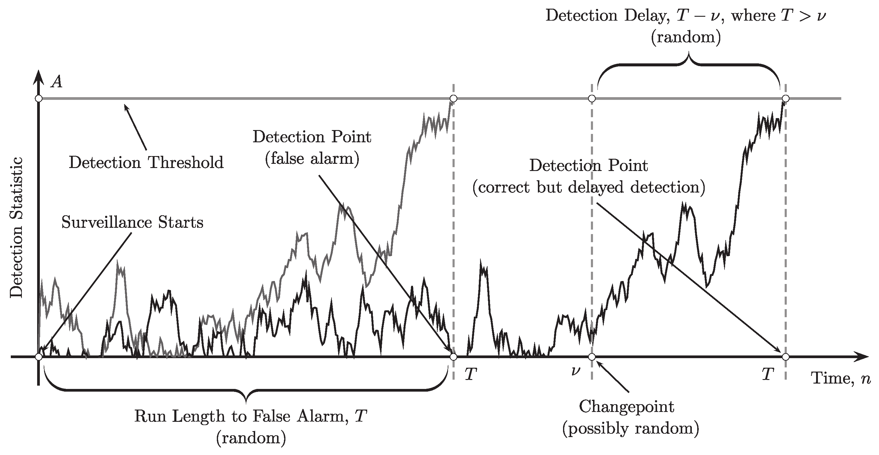
as Figure 1 suggests, the risk associated with a true change detection is reasonable to measure by the conditional average delay to detection

$${\mathsf{CEDD}}_{\nu }\left(T\right)={\mathsf{E}}_{\nu }[T-\nu |T>\nu ],\nu =0,1,\cdots ,$$

but not necessarily by the ARL to detection ${\mathsf{E}}_0\left[T\right]\equiv {\mathsf{CEDD}}_0\left(T\right)$. A good detection procedure should guarantee small values of the expected detection delay ${\mathsf{CEDD}}_{\nu }\left(T\right)$ for all change points $\nu \ge 0$ when $\mathsf{ARL}\mathsf{2}\mathsf{FA}\left(T\right)$ is fixed at a certain level. However, if the false alarm risk is measured in terms of the ARL to false alarm, i.e., it is required that $\mathsf{ARL}\mathsf{2}\mathsf{FA}\left(T\right)\ge \gamma$ for some $\gamma \ge 1$, then a procedure that minimizes the conditional average delay to detection ${\mathsf{CEDD}}_{\nu }\left(T\right)$ uniformly over all $\nu$ does not exist. For this reason, we have to resort to different optimality criteria, e.g., to Bayesian and minimax criteria.

Minimax Changepoint Optimization Criteria 

There are two popular minimax criteria. The first one was introduced by Lorden [47]:

$$\underset{T}{inf}\underset{\nu \ge 0}{sup}ess\; sup{\mathsf{E}}_{\nu }[T-\nu \mid T>\nu ,{\mathcal{F}}_{\nu }]\mathrm{subject}\mathrm{to}\mathsf{ARL}\mathsf{2}\mathsf{FA}\left(T\right)\ge \gamma .$$

It requires minimizing the conditional expected delay to detection ${\mathsf{E}}_{\nu }[T-\nu \mid T>\nu ,{\mathcal{F}}_{\nu }]$ in the worst-case scenario with respect to both the change point $\nu$ and the trajectory $(X_1,\cdots ,X_{\nu })$ of the observed process in the class of detection procedures

$${\mathbb{C}}_{\mathrm{ARL}}\left(\gamma \right)=\left\{T:\mathsf{ARL}\mathsf{2}\mathsf{FA}\left(T\right)\ge \gamma \right\},\gamma \ge 1,$$

for which the ARL to false alarm exceeds the prespecified value $\gamma \in [1,\infty )$. Let $\mathsf{ESADD}\left(T\right)={sup}_{\nu \ge 0}ess\; sup{\mathsf{E}}_{\nu }[T-\nu \mid T>\nu ,{\mathcal{F}}_{\nu }]$ denote Lorden’s speed detection measure. Under Lorden’s minimax approach the goal is to find a stopping time $T_{\mathrm{opt}}\in {\mathbb{C}}_{\mathrm{ARL}}\left(\gamma \right)$ such that

$$\mathsf{ESADD}\left(T_{\mathrm{opt}}\right)=\underset{T\in {\mathbb{C}}_{\mathrm{ARL}}\left(\gamma \right)}{inf}\mathsf{ESADD}\left(T\right)\mathrm{for}\mathrm{any}\gamma \ge 1.$$

In the classical i.i.d. scenario (53), Lorden [47] proved that the CUSUM detection procedure (55) is asymptotically first-order minimax optimal as $\gamma \to \infty$, i.e.,

$$\underset{T\in {\mathbb{C}}_{\mathrm{ARL}}\left(\gamma \right)}{inf}\mathsf{ESADD}\left(T\right)=\mathsf{ESADD}\left({\mathsf{T}}_{\mathsf{CS}}\right)(1+o\left(1\right)),\gamma \to \infty .$$

Later on, Moustakides [48], using optimal stopping theory, in his ingenious paper established the exact optimality of CUSUM for any ARL to false alarm $\gamma \ge 1$.

Another popular, less pessimistic minimax criterion is due to Pollak [49]:

$$\underset{T}{inf}\underset{\nu \ge 0}{sup}{\mathsf{CEDD}}_{\nu }\left(T\right)\mathrm{subject}\mathrm{to}\mathsf{ARL}\mathsf{2}\mathsf{FA}\left(T\right)\ge \gamma ,$$

which requires minimizing the conditional expected delay to detection ${\mathsf{CEDD}}_{\nu }\left(T\right)={\mathsf{E}}_{\nu }[T-\nu \mid T>\nu ]$ in the worst-case scenario with respect to the change point $\nu$ in class ${\mathbb{C}}_{\mathrm{ARL}}\left(\gamma \right)$. Under Pollak’s minimax approach the goal is to find a stopping time $T_{\mathrm{opt}}\in {\mathbb{C}}_{\mathrm{ARL}}\left(\gamma \right)$ such that

$$\underset{\nu \ge 0}{sup}{\mathsf{CEDD}}_{\nu }\left(T_{\mathrm{opt}}\right)=\underset{T\in {\mathbb{C}}_{\mathrm{ARL}}\left(\gamma \right)}{inf}\underset{\nu \ge 0}{sup}{\mathsf{CEDD}}_{\nu }\left(T\right)\mathrm{for}\mathrm{any}\gamma \ge 1.$$

For the i.i.d. model (53), Pollak [49] showed that the modified SR detection procedure that starts from the quasi-stationary distribution of the SR statistic (i.e., the head-start $r_0$ in the SR-r procedure is a specific random variable) is third-order asymptotically optimal as $\gamma \to \infty$, i.e., the best one can attain up to an additive term $o\left(1\right)$:

$$\underset{T\in {\mathbb{C}}_{\mathrm{ARL}}\left(\gamma \right)}{inf}\underset{\nu \ge 0}{sup}{\mathsf{CEDD}}_{\nu }\left(T\right)=\underset{\nu \ge 0}{sup}{\mathsf{CEDD}}_{\nu }\left({\mathsf{T}}_{\mathsf{SR}}^{{\mathsf{r}}_{\mathsf{0}}}\right)+o\left(1\right),\gamma \to \infty ,$$

where $o\left(1\right)\to 0$ as $\gamma \to \infty$. Later Tartakovsky et al. [50] proved that this is also true for the SR-r procedure (62) that starts from the fixed but specially designed point $r_0=r_0\left(\gamma \right)$ that depends on $\gamma$, which was first introduced and thoroughly studied by Moustakides et al. [45]. See also Polunchenko and Tartakovsky [51] on the exact optimality of the SR-r procedure.

Bayesian Changepoint Optimization Criterion 

In Bayesian problems, the point of change $\nu$ is treated as random with a prior distribution ${\pi }_k=Pr(\nu =k)$, $-\infty <k<+\infty$. Define the probability measure on the Borel $\sigma$-algebra $\mathcal{B}$ in ${\mathbb{R}}^{\infty }\times \mathbb{N}$ as

$${\mathsf{P}}^{\pi }(\mathcal{A}\times \mathcal{K})=\sum _{k\in \mathcal{K}}{\pi }_k{\mathsf{P}}_k\left(\mathcal{A}\right),\mathcal{A}\in \mathcal{B}\left({\mathbb{R}}^{\infty }\right),\mathcal{K}\in \mathbb{N}.$$

Under measure ${\mathsf{P}}^{\pi }$ the change point $\nu$ has distribution $\pi =\left\{{\pi }_k\right\}$ and the model for the observations is given in (52). From the Bayesian point of view, it is reasonable to measure the false alarm risk with the Weighted Probability of False Alarm (PFA), defined as

$${\mathsf{PFA}}^{\pi }\left(T\right):={\mathsf{P}}^{\pi }(T\le \nu )=\sum _{k=-\infty }^{\infty }{\pi }_k{\mathsf{P}}_k(T\le k)=\sum _{k=0}^{\infty }{\pi }_k{\mathsf{P}}_{\infty }(T\le k).$$

(63)

The summation in (63) is over $k\in {\mathbb{Z}}_{+}=\{0,1,2,\cdots \}$ since ${\mathsf{P}}_{\infty }(T<0)=0$. Also, the last equality follows from the fact that ${\mathsf{P}}_k(T\le k)={\mathsf{P}}_{\infty }(T\le k)$ because the event $\{T\le k\}$ depends on the first k observations which under measure ${\mathsf{P}}_k$ correspond to the no-change hypothesis ${\mathsf{H}}_{\infty }$. Thus, for $\alpha \in (0,1)$, introduce the class of changepoint detection procedures

$${\mathbb{C}}_{\pi }\left(\alpha \right)=\left\{T:{\mathsf{PFA}}^{\pi }\left(T\right)\le \alpha \right\}$$

(64)

for which the weighted PFA does not exceed a prescribed level $\alpha$. Let ${\mathsf{E}}^{\pi }$ denote expectation with respect to measure ${\mathsf{P}}^{\pi }$.

Shiryaev [18,44] introduced the Bayesian optimality criterion

$$\underset{T\in {\mathbb{C}}_{\pi }\left(\alpha \right)}{inf}{\mathsf{E}}^{\pi }\left[{(T-\nu )}^{+}\right],$$

which is equivalent to minimizing the conditional average detection delay ${\mathsf{EDD}}^{\pi }\left(T\right)={\mathsf{E}}^{\pi }[T-\nu |T>\nu ]$

$$\underset{T}{inf}{\mathsf{EDD}}^{\pi }\left(T\right)\mathrm{subject}\mathrm{to}{\mathsf{PFA}}^{\pi }\left(T\right)\le \alpha .$$

Under the Bayesian approach, the goal is to find a stopping time $T_{\mathrm{opt}}\in {\mathbb{C}}_{\pi }\left(\alpha \right)$ such that

$${\mathsf{EDD}}^{\pi }\left(T_{\mathrm{opt}}\right)=\underset{T\in {\mathbb{C}}_{\pi }\left(\alpha \right)}{inf}{\mathsf{EDD}}^{\pi }\left(T\right)\mathrm{for}\mathrm{any}\alpha \in (0,1).$$

(65)

For the i.i.d. model (53) and under the assumption that the changepoint $\nu$ has the zero-modified geometric prior distribution $\mathrm{Geometric}(p,\varrho )$ (59), this problem was solved by Shiryaev [18,44]. Shiryaev [18,44,52] proved that the optimal detection procedure is based on comparing the posterior probability of a change currently being in effect with a certain detection threshold, which is equivalent to the stopping time ${\mathsf{T}}_{\mathsf{SH}}\left(A\right)$ (57). To guarantee its strict optimality the detection threshold $A=A_{\alpha }$ should be set to guarantee that the PFA is exactly equal to the selected level $\alpha$. Thus, if $A=A_{\alpha }$ can be selected in such a way that ${\mathsf{PFA}}^{\pi }\left({\mathsf{T}}_{\mathsf{SH}}\left(A_{\alpha }\right)\right)=\alpha$, then it is strictly optimal in class ${\mathbb{C}}_{\pi }\left(\alpha \right)$,

$$\underset{T\in {\mathbb{C}}_{\pi }\left(\alpha \right)}{inf}{\mathsf{EDD}}^{\pi }\left(T\right)={\mathsf{EDD}}^{\pi }\left({\mathsf{T}}_{\mathsf{SH}}\left(A_{\alpha }\right)\right)\mathrm{for}\mathrm{any}0<\alpha <1-p.$$

Uniform Optimality Under Local Probabilities of False Alarm 

While the Bayesian and minimax formulations are reasonable and can be justified in many applications, it would be most desirable to guarantee small values of the conditional expected detection delay ${\mathsf{CEDD}}_{\nu }\left(T\right)={\mathsf{E}}_{\nu }[T-\nu |T\ge \nu ]$ uniformly for all $\nu \in {\mathbb{Z}}_{+}$ when the false alarm risk is fixed at a certain level. However, as we already mentioned, if the false alarm risk is measured in terms of the ARL to false alarm, i.e. if it is required that $\mathsf{ARL}\mathsf{2}\mathsf{FA}\left(T\right)\ge \gamma$ for some $\gamma \ge 1$, then a procedure that minimizes ${\mathsf{CEDD}}_{\nu }\left(T\right)$ for all $\nu$ does not exist. More importantly, as discussed in [5], the requirement of having large values of the $\mathsf{ARL}\mathsf{2}\mathsf{FA}\left(T\right)$ generally does not guarantee small values of the maximal local probability of false alarm $\mathsf{MLPFA}\left(T\right)={sup}_{\ell \ge 0}{\mathsf{P}}_{\infty }(T\le \ell +m|T>\ell )$ in a time window of a length $m\ge 1$, while the opposite is always true (see Lemmas 2.1-2.2 in [5]). Hence, the constraint $\mathsf{MLPFA}\left(T\right)\le \beta$ is more stringent than $\mathsf{ARL}\mathsf{2}\mathsf{FA}\left(T\right)\ge \gamma$.

Yet another reason for considering the MLPFA constraint instead of the ARL to false alarm constraint is that the latter one makes sense, if and only if, the ${\mathsf{P}}_{\infty }$-distribution of stopping times is geometric or at least close to geometric, which is often the case for many popular detection procedures such as CUSUM and SR in the i.i.d. case. However, for general non-i.i.d. models this is not necessarily true (see [5] and [53] for a detailed discussion).

For these reasons, introduce the most stringent class of change detection procedures for which the $\mathsf{MLPFA}\left(T\right)$ is upper-bounded by the prespecified level $\beta \in (0,1)$:

$${\mathbb{C}}_{\mathrm{PFA}}(m,\beta )=\left\{T:\underset{\ell \ge 0}{sup}{\mathsf{P}}_{\infty }(T\le \ell +m|T>\ell )\le \beta \right\}.$$

(66)

The goal is to find a stopping time $T_{\mathrm{opt}}\in {\mathbb{C}}_{\mathrm{PFA}}(m,\beta )$ such that

$${\mathsf{CEDD}}_{\nu }\left(T_{\mathrm{opt}}\right)=\underset{T\in {\mathbb{C}}_{\mathrm{PFA}}(m,\beta )}{inf}{\mathsf{CEDD}}_{\nu }\left(T\right)\mathrm{for}\mathrm{all}\nu \in {\mathbb{Z}}_{+}\mathrm{and}\mathrm{any}0<\beta <1.$$

(67)

3.2.4. Asymptotic Optimality for General Non-i.i.d. Models via r-Quick and r-Complete Convergence

Complete Convergence and General Bayesian Changepoint Detection Theory 

Consider first the Bayesian problem assuming that the change point $\nu$ is a random variable independent of the observations with a prior distribution $\pi =\left\{{\pi }_k\right\}$. Unfortunately, in the general non-i.i.d. case and for an arbitrary prior $\pi$, the Bayesian optimization problem (65) is intractable for arbitrary values of PFA $\alpha \in (0,1)$. For this reason, we will consider the following first-order asymptotic problem assuming that the given PFA $\alpha$ approaches zero: Find a change detection procedure $T^{*}$ such that it minimizes the expected detection delay ${\mathsf{EDD}}^{\pi }\left(T\right)$ asymptotically to first order as $\alpha \to 0$. That is, the goal is to design such a detection procedure $T^{*}$ that

$$\underset{T\in {\mathbb{C}}_{\pi }\left(\alpha \right)}{inf}{\mathsf{EDD}}^{\pi }\left(T\right)={\mathsf{EDD}}^{\pi }\left(T^{*}\right)(1+o\left(1\right))\mathrm{as}\alpha \to 0,$$

(68)

where $o\left(1\right)\to 0$ as $\alpha \to 0$. It turns out that in the asymptotic setting, it is also possible to find a procedure that minimizes the conditional expected detection delay ${\mathsf{EDD}}_k\left(T\right)={\mathsf{E}}_k\left[T-k|T>k\right]$ uniformly for all possible values of the change point $\nu =k\in {\mathbb{Z}}_{+}$, i.e.,

$$\underset{\alpha \to 0}{lim}\frac{{inf}_{T\in {\mathbb{C}}_{\pi }\left(\alpha \right)}{\mathsf{EDD}}_k\left(T\right)}{{\mathsf{EDD}}_k\left(T^{*}\right)}=1\mathrm{for}\mathrm{all}k\in {\mathbb{Z}}_{+}.$$

(69)

Note that if the change occurs before the observations become available, i.e., $\nu =k\in \{-1,-2,\cdots \}$, then ${\mathsf{EDD}}_k\left(T\right)\equiv {\mathsf{E}}_0\left[T\right]$ since $T\ge 0$ w.p. 1.

Furthermore, asymptotic optimality results can be also established for higher moments of the detection delay of order $r>1$

$${\mathsf{E}}_k\left[{(T-k)}^r|T>k\right]\mathrm{and}{\mathsf{E}}^{\pi }\left[{(T-\nu )}^r|T>\nu \right].$$

Since the Shiryaev procedure ${\mathsf{T}}_{\mathsf{SH}}\left(A\right)$ defined in (57)-(58) is optimal for the i.i.d. model and $\mathrm{Geometric}(p,\varrho )$ prior, it is reasonable to assume that it is asymptotically optimal for the more general prior and the non-i.i.d model. However, to study asymptotic optimality we need certain constraints imposed on the prior distribution and on the asymptotic behavior of the decision statistics as the sample size increases, i.e., on the general stochastic model (52).

Assume that the prior distribution $\left\{{\pi }_k\right\}$ is fully supported, i.e., ${\pi }_k>0$ for all $k\in {\mathbb{Z}}_{+}$ and ${\pi }_{\infty }=0$ and that the following conditions hold:

$$\underset{n\to \infty }{lim}\frac{1}{n}\left|log\sum _{k=n+1}^{\infty }{\pi }_k\right|=\mu \mathrm{for}\mathrm{some}0\le \mu <\infty ;$$

(70)

$$\sum _{k=0}^{\infty }{\pi }_k{|log{\pi }_k|}^r<\infty \mathrm{for}\mathrm{some}r\ge 1\mathrm{if}\mu =0.$$

(71)

Note that if $\mu >0$, then by condition (70) the prior distribution has an exponential right tail. Distributions such as geometric and discrete versions of gamma and logistic distributions, i.e., models with bounded hazard rates, belong to this class. In this case, condition (71) holds automatically. If $\mu =0$, the distribution has a heavy tail, i.e., belongs to the model with a vanishing hazard rate. However, we cannot allow this distribution to have a too-heavy tail, which is guaranteed by condition (71).

Define the LLR of the hypotheses ${\mathsf{H}}_k$ and ${\mathsf{H}}_{\infty }$

$${\lambda }_n^k=log\frac{\mathrm{d}{\mathsf{P}}_k^{\left(n\right)}}{\mathrm{d}{\mathsf{P}}_{\infty }^{\left(n\right)}}=\sum _{t=k+1}^n\frac{f_t\left(X_t\right|{\mathbf{X}}^t)}{g_t\left(X_t\right|{\mathbf{X}}^t)},n>k$$

(${\lambda }_n^k=0$ for $n\le k$). To obtain asymptotic optimality results the general non-i.i.d. model for observations is restricted to the case that the normalized LLR $n^{-1}{\lambda }_{k+n}^k$ obeys the SLLN as $n\to \infty$ with a finite and positive number I under the probability measure ${\mathsf{P}}_k$ and its r-complete strengthened version

$$\sum _{n=1}^{\infty }{n}^{r-1}\underset{k\in {\mathbb{Z}}_{+}}{sup}{\mathsf{P}}_k\left\{|n^{-1}{\lambda }_{k+n}^k-I|>\epsilon \right\}<\infty \mathrm{for}\mathrm{every}\epsilon >0.$$

(72)

By Lemma 7.2.1 in [6],

$${\mathsf{PFA}}^{\pi }\left({\mathsf{T}}_{\mathsf{SH}}\left(A\right)\right)\le 1/(1+A)\mathrm{for}\mathrm{every}A>p/(1-p),$$

and therefore, setting $A=A_{\alpha }=(1-\alpha )/\alpha$ guarantees that ${\mathsf{T}}_{\mathsf{SH}}\left(A_{\alpha }\right)\in {\mathbb{C}}_{\pi }\left(\alpha \right)$.

The following theorem that can be deduced from Theorem 3.7 in [5] shows that the Shiryaev detection procedure is asymptotically optimal if the normalized LLR $n^{-1}{\lambda }_{k+n}^k$ converges r-completely to a positive and finite number I and the prior distribution satisfies conditions (70)-(71).

Theorem 6.

Let $r\ge 1$. Let the prior distribution of the change point satisfy conditions (70)-(71). Assume that there exists some number $0<I<\infty$ such that the LLR process $n^{-1}{\lambda }_{k+n}^k$ converges to I uniformly completely as $n\to \infty$ under ${\mathsf{P}}_k$, i.e., condition (72) holds. If threshold $A=A_{\alpha }$ in the Shiryaev procedure is so selected that ${\mathsf{PFA}}^{\pi }\left({\mathsf{T}}_{\mathsf{SH}}\left(A_{\alpha }\right)\right)\le \alpha$ and $log{A}_{\alpha }\sim |log\alpha |$ as $\alpha \to 0$, e.g., as $A=(1-\alpha )/\alpha$, then as $\alpha \to 0$

$$\begin{array}{c}\hfill \underset{T\in {\mathbb{C}}_{\pi }\left(\alpha \right)}{inf}{\mathsf{E}}_k\left[{(T-k)}^r|T>k\right]\sim {\left(\frac{|log\alpha |}{I+\mu }\right)}^r\sim {\mathsf{E}}_k\left[{({\mathsf{T}}_{\mathsf{SH}}-k)}^r|{\mathsf{T}}_{\mathsf{SH}}>k\right]\mathrm{for}\mathrm{all}k\in {\mathbb{Z}}_{+}\end{array}$$

and

$$\underset{T\in {\mathbb{C}}_{\pi }\left(\alpha \right)}{inf}{\mathsf{E}}^{\pi }\left[{(T-\nu )}^r|T>\nu \right]\sim {\left(\frac{|log\alpha |}{I+\mu }\right)}^r\sim {\mathsf{E}}^{\pi }\left[{({\mathsf{T}}_{\mathsf{SH}}-\nu )}^r|{\mathsf{T}}_{\mathsf{SH}}>\nu \right].$$

Therefore, the Shiryaev procedure ${\mathsf{T}}_{\mathsf{SH}}\left(A_{\alpha }\right)$ is first-order asymptotically optimal as $\alpha \to 0$ in class ${\mathbb{C}}_{\pi }\left(\alpha \right)$, minimizing moments of the detection delay up to order r whenever the r-complete version of the SLLN (72) holds for the LLR process.

For $r=1$, the assertions of this theorem imply asymptotic optimality of the Shiryaev procedure for the expected detection delays (68) and (69) as well as asymptotic approximations for the expected detection delays.

Remark 7.

The results of Theorem 6 can be generalized to the asymptotically non-stationary case where ${\lambda }_{k+n}^k/\psi \left(n\right)$ converges to I uniformly completely as $n\to \infty$ under ${\mathsf{P}}_k$ with a non-linear function $\psi \left(n\right)$ similarly to the hypothesis testing problem discussed in Section 3.1. See also the recent paper [54] for the minimax change detection problem with independent but substantially non-stationary post-change observations.

It is also interesting to see how two other most popular changepoint detection procedures – the SR and CUSUM – perform in the Bayesian context.

Consider the SR-r procedure defined by (61)-(62). It follows from Lemma 3.4 (page 100) in [5] that

$${\mathsf{PFA}}^{\pi }\left({\mathsf{T}}_{\mathsf{SR}}^{{\mathsf{r}}_{\mathsf{0}}}\left(A\right)\right)\le \frac{r_0{\sum }_{k=1}^{\infty }{\pi }_k+{\sum }_{k=1}^{\infty }k{\pi }_k}{A}\mathrm{for}\mathrm{every}A>0,$$

and therefore, setting $A=A_{\alpha }={\alpha }^{-1}(r_0+{\sum }_{k=1}^{\infty }k{\pi }_k)$ implies ${\mathsf{T}}_{\mathsf{SR}}^{{\mathsf{r}}_{\mathsf{0}}}\left(A_{\alpha }\right)\in {\mathbb{C}}_{\pi }\left(\alpha \right)$. Let threshold $A=A_{\alpha }$ in the SR-r procedure is so selected that ${\mathsf{PFA}}_{\pi }\left({\mathsf{T}}_{\mathsf{SR}}^{{\mathsf{r}}_{\mathsf{0}}}\left(A_{\alpha }\right)\right)\le \alpha$ and $log{A}_{\alpha }\sim |log\alpha |$ as $\alpha \to 0$, e.g., as $A_{\alpha }={\alpha }^{-1}(r_0+{\sum }_{k=1}^{\infty }k{\pi }_k)$, then as $\alpha \to 0$

$$\begin{array}{c}\hfill {\mathsf{E}}_k\left[{({\mathsf{T}}_{\mathsf{SR}}^{{\mathsf{r}}_{\mathsf{0}}}-k)}^r|{\mathsf{T}}_{\mathsf{SR}}^{{\mathsf{r}}_{\mathsf{0}}}>k\right]\sim {\left(\frac{|log\alpha |}{I}\right)}^r\mathrm{for}\mathrm{all}k\in {\mathbb{Z}}_{+}\end{array}$$

(73)

and

$${\mathsf{E}}^{\pi }\left[{({\mathsf{T}}_{\mathsf{SR}}^{{\mathsf{r}}_{\mathsf{0}}}-\nu )}^r|{\mathsf{T}}_{\mathsf{SR}}^{{\mathsf{r}}_{\mathsf{0}}}>\nu \right]\sim {\left(\frac{|log\alpha |}{I}\right)}^r$$

(74)

whenever the uniform r-complete convergence condition (72) holds. Therefore, the SR-r procedure ${\mathsf{T}}_{\mathsf{SR}}^{{\mathsf{r}}_{\mathsf{0}}}\left(A_{\alpha }\right)$ is first-order asymptotically optimal as $\alpha \to 0$ in class ${\mathbb{C}}_{\pi }\left(\alpha \right)$, minimizing moments of the detection delay up to order r, when the prior distribution $\pi$ is heavy-tailed (i.e., when $\mu =0$) and the r-complete version of the SLLN holds. In the case where $\mu >0$ (i.e., the prior distribution has an exponential tail) the SR-r procedure is not optimal. This can be expected since it uses the improper uniform prior in the detection statistic.

The same asymptotic results (73)-(74) are true for the CUSUM procedure ${\mathsf{T}}_{\mathsf{CS}}\left(a\right)$ defined in (55) if threshold $a=a_{\alpha }$ is so selected that ${\mathsf{PFA}}_{\pi }\left({\mathsf{T}}_{\mathsf{CS}}\left(a_{\alpha }\right)\right)\le \alpha$ and $a_{\alpha }\sim |log\alpha |$ as $\alpha \to 0$ and the uniform r-complete convergence condition (72) holds.

Hence, the r-complete convergence of the LLR process is the sufficient condition for uniform asymptotic optimality of several popular change detection procedures in class ${\mathbb{C}}_{\pi }\left(\alpha \right)$.

Complete Convergence and General Non-Bayesian Changepoint Detection Theory 

Consider now the non-Bayesian problem assuming that the change point $\nu$ is an unknown deterministic number. We focus on the most interesting for applications uniform optimality criterion (67) that requires minimizing the conditional expected delay to detection ${\mathsf{CEDD}}_{\nu }\left(T\right)={\mathsf{E}}_{\nu }[T-\nu |T>\nu ]$ for all values of the change point $\nu \in {\mathbb{Z}}_{+}$ in the class of change detection procedures ${\mathbb{C}}_{\mathrm{PFA}}(m,\beta )$ defined in (66). Recall that this class includes change detection procedures with the maximal local probability of false alarm in the time window m,

$$\mathsf{MLPFA}\left(T\right)=\underset{\ell \ge 0}{sup}{\mathsf{P}}_{\infty }(T\le \ell +m|T>\ell ),$$

which does not exceed the prescribed value $\beta \in (0,1)$. However, the exact solution to this challenging problem is unknown even in the i.i.d. case.

So instead consider the following asymptotic problem assuming that the given MLPFA $\beta$ goes to zero: Find a change detection procedure $T^{★}$ which minimizes the expected detection delay ${\mathsf{E}}_{\nu }[T-\nu |T>\nu ]$ asymptotically to first order as $\beta \to 0$. That is, the goal is to design such a detection procedure $T^{★}$ that

$$\underset{T\in {\mathbb{C}}_{\mathrm{PFA}}(m,\beta )}{inf}{\mathsf{E}}_{\nu }[T-\nu |T>\nu ]={\mathsf{E}}_{\nu }[T^{★}-\nu |T^{★}>\nu ](1+o\left(1\right))\mathrm{for}\mathrm{all}\nu \in {\mathbb{Z}}_{+}\mathrm{as}\beta \to 0.$$

More generally, we may focus on the asymptotic problem of minimizing moments of the detection delay of order $r\ge 1$:

$$\underset{T\in {\mathbb{C}}_{\mathrm{PFA}}(m,\beta )}{inf}{\mathsf{E}}_{\nu }\left[{(T-\nu )}^r\right|T>\nu ]={\mathsf{E}}_{\nu }\left[{(T^{★}-\nu )}^r\right|T^{★}>\nu ](1+o\left(1\right))\mathrm{for}\mathrm{all}\nu \in {\mathbb{Z}}_{+}\mathrm{as}\beta \to 0.$$

To solve this problem we need to assume that the window length $m=m_{\beta }$ is a function of the MLPFA constraint $\beta$ and that $m_{\beta }$ goes to infinity as $\beta \to 0$ with a certain appropriate rate. Using [55] the following results can be established.

Let $r\ge 1$ and assume that the complete version of the SLLN holds with some number $0<I<\infty$, i.e., $n^{-1}{\lambda }_{\nu +n}^{\nu }$ converges to I uniformly completely as $n\to \infty$ under ${\mathsf{P}}_{\nu }$. If $m_{\beta }={O\left(\right|log\beta |}^2)$ as $\beta \to \infty$ and threshold $A=A_{\beta }$ in the SR procedure is so selected that $\mathsf{MPFA}\left({\mathsf{T}}_{\mathsf{SR}}\left(A_{\beta }\right)\right)\le \beta$ and $log{A}_{\beta }\sim |log\beta |$ as $\beta \to 0$, e.g., as defined in [55], then as $\beta \to 0$

$$\begin{array}{c}\hfill \underset{T\in {\mathbb{C}}_{\mathrm{PFA}}(m_{\beta },\beta )}{inf}{\mathsf{E}}_{\nu }\left[{(T-\nu )}^r|T>\nu \right]\sim {\left(\frac{|log\beta }{I}\right)}^r\sim {\mathsf{E}}_{\nu }\left[{({\mathsf{T}}_{\mathsf{SR}}-\nu )}^r|{\mathsf{T}}_{\mathsf{SR}}>\nu \right]\mathrm{for}\mathrm{all}\nu \in {\mathbb{Z}}_{+}.\end{array}$$

A similar result also holds for the CUSUM procedure ${\mathsf{T}}_{\mathsf{CS}}\left(a\right)$ if threshold $a=a_{\beta }$ is so selected that $\mathsf{MPFA}\left({\mathsf{T}}_{\mathsf{CS}}\left(a_{\beta }\right)\right)\le \beta$ and $a_{\beta }\sim |log\beta |$ as $\beta \to 0$ and the complete version of the SLLN holds for the normalized LLR $n^{-1}{\lambda }_{\nu +n}^{\nu }$ as $n\to \infty$.

Hence, the r-complete convergence of the LLR process is the sufficient condition for uniform asymptotic optimality of SR and CUSUM change detection procedures with respect to moments of the detection delay of order r in class ${\mathbb{C}}_{\mathrm{PFA}}(m_{\beta },\beta )$.

4. Quick and Complete Convergence for Markov and Hidden Markov Models

Usually, in particular problems, verification of the SLLN for the LLR process is relatively easy. However, in practice, verifying strengthened r-complete or r-quick versions of the SLLN, i.e., checking condition (72) can cause some difficulty. Many interesting examples where this verification was performed can be found in [5,6]. However, it is interesting to find sufficient conditions for r-complete convergence for a relatively large class of stochastic models.

In this section, we outline this issue for Markov and hidden Markov models based on the results obtained by Pergamenchtchikov and Tartakovsky [55] for ergodic Markov processes and by Fuh and Tartakovsky [56] for hidden Markov models (HMM). See also Tartakovsky [5].

Let ${\left\{X_n\right\}}_{n\in {\mathbb{Z}}_{+}}$ be a time-homogeneous Markov process with values in a measurable space $(\mathcal{X},\mathcal{B})$ with the transition probability $P(x,A)$. Let ${\mathsf{E}}_x$ denote the expectation with respect to this probability. Assume that this process is geometrically ergodic, i.e., there exist positives constants $0<R<\infty$, $\kappa >0$, probability measure $\varkappa$ on $(\mathcal{X},\mathcal{B})$ and the Lyapunov $\mathcal{X}\to [1,\infty )$ function V with $\varkappa \left(V\right)<\infty$, such that

$$\underset{n\in {\mathbb{Z}}_{+}}{sup}{e}^{\kappa n}\underset{0<\psi \le V}{sup}\underset{x}{sup}\frac{1}{V\left(x\right)}\left|{\mathsf{E}}_x\left[\psi \left(X_n\right)\right]-\varkappa \left(\psi \right)\right|\le R.$$

In the change detection problem, the sequence ${\left\{X_n\right\}}_{n\in {\mathbb{Z}}_{+}}$ is a Markov process, such that ${\left\{X_n\right\}}_{1\le n\le \nu }$ is a homogeneous process with the transition density $g\left(y\right|x)$ and ${\left\{X_n\right\}}_{n>\nu }$ is homogeneous positive ergodic with the transition density $f_{(}y\left|x\right)$ and the ergodic (stationary) distribution $\varkappa$. In this case, the LLR process ${\lambda }_n^k$ can be represented as

$${\lambda }_n^k=\sum _{t=k+1}^{n}G(X_t,X_{t-1}),n>k,$$

where $G(y,x)=log\left[f\right(y\left|x\right)/g\left(y\right|x\left)\right]$.

Define

$$I={\int }_{\mathcal{X}}\left\{{\int }_{\mathcal{X}}G(y,x)f\left(y\right|x)\mathrm{d}y\right\}\varkappa \left(\mathrm{d}x\right).$$

Under a set of quite sophisticated sufficient conditions the LLR ${\lambda }_{k+n}^n/n$ converges r-completely to I (cf. [55]). We omit the details and only mention that the main condition is the finiteness of $(r+1)$-th moment of the LLR increment, ${\mathsf{E}}_0\left[{\left(G(X_1,X_0)\right)}^{r+1}\right]<\infty$.

Consider now the HMM with finite state space. Then again, as in the pure Markov case, the main condition for r-complete convergence of ${\lambda }_{k+n}^n/n$ to I , where I is specified in Fuh and Tartakovsky [56], is ${\mathsf{E}}_0\left[{\left({\lambda }_1^0\right)}^{r+1}\right]<\infty$. Further details can be found in [56].

Similar results for Markov and hidden Markov models hold for the hypothesis testing problem considered in Section 3.1. Specifically, if in the Markov case we assume that the observed Markov process ${\left\{X_n\right\}}_{n\in {\mathbb{Z}}_{+}}$ is a time-homogeneous geometrically ergodic with transition density $f_i\left(y\right|x)$ under hypothesis ${\mathsf{H}}_i$ ($i=0,1,\cdots ,N$) and invariant distribution ${\varkappa }_i$, then the LLR processes are

$${\lambda }_{ij}\left(n\right)=\sum _{t=1}^n{G}_{ij}(X_t,X_{t-1}),i,j=0,1,\cdots ,N,i\ne j,$$

where $G_{ij}(y,x)=log[f_i\left(y\right|x)/f_j\left(y\right|x)]$. If ${\mathsf{E}}_i\left[{\left(G_{ij}(X_1,X_0)\right)}^{r+1}\right]<\infty$ then the LLR $n^{-1}{\lambda }_{ij}\left(n\right)$ converges r-completely to a finite number

$$I_{ij}={\int }_{\mathcal{X}}\left\{{\int }_{\mathcal{X}}{G}_{ij}(y,x)f_i\left(y\right|x)\mathrm{d}y\right\}{\varkappa }_i\left(\mathrm{d}x\right).$$

5. Conclusion

We show that the strengthened versions of the SLLN, specifically the r-quick and r-complete versions, are useful tools for many statistical problems for general non-i.i.d. stochastic models. In particular, r-quick and r-complete convergences for log-likelihood ratio processes are sufficient for near optimality of sequential hypothesis tests and changepoint detection procedures for models with dependent and non-identically distributed observations. Such non-i.i.d. models are typical for modern large-scale information and physical systems that produce Big Data in numerous practical applications. Readers interested in specific applications may find detailed discussions in [4,5,6,8,19,22,23,34,36,38,54,55,56,57,58,59,54].

References

- Hsu, P.L.; Robbins, H. Complete convergence and the law of large numbers. Proceedings of the National Academy of Sciences of the United States of America 1947, 33, 25–31. [CrossRef]
- Baum, L.E.; Katz, M. Convergence rates in the law of large numbers. Transactions of the American Mathematical Society 1965, 120, 108–123. [CrossRef]
- Strassen, V. Almost sure behavior of sums of independent random variables and martingales. In Proceedings of the Fifth Berkeley Symposium on Mathematical Statistics and Probability, June 21–July 18, 1965 and December 27, 1965–January 7, 1966; Le Cam, L.M.; Neyman, J., Eds.; University of California Press: Berkeley, CA, USA, 1967; Vol. 2: Contributions to Probability Theory. Part 1, pp. 315–343.
- Tartakovsky, A.G. Asymptotic optimality of certain multihypothesis sequential tests: Non-i.i.d. case. Statistical Inference for Stochastic Processes 1998, 1, 265–295. [CrossRef]
- Tartakovsky, A.G. Sequential Change Detection and Hypothesis Testing: General Non-i.i.d. Stochastic Models and Asymptotically Optimal Rules; Monographs on Statistics and Applied Probability 165, Chapman & Hall/CRC Press, Taylor & Francis Group: Boca Raton, London, New York, 2020.
- Tartakovsky, A.G.; Nikiforov, I.V.; Basseville, M. Sequential Analysis: Hypothesis Testing and Changepoint Detection; Monographs on Statistics and Applied Probability 136, Chapman & Hall/CRC Press, Taylor & Francis Group: Boca Raton, London, New York, 2015.
- Lai, T.L. On r-quick convergence and a conjecture of Strassen. Annals of Probability 1976, 4, 612–627.
- Lai, T.L. Asymptotic optimality of invariant sequential probability ratio tests. Annals of Statistics 1981, 9, 318–333. [CrossRef]
- Chow, Y.S.; Lai, T.L. Some one-sided theorems on the tail distribution of sample sums with applications to the last time and largest excess of boundary crossings. Transactions of the American Mathematical Society 1975, 208, 51–72. [CrossRef]
- Fuh, C.D.; Zhang, C.H. Poisson equation, moment inequalities and quick convergence for Markov random walks. Stochastic Processes and Their Applications 2000, 87, 53–67. [CrossRef]
- Wald, A. Sequential tests of statistical hypotheses. Annals of Mathematical Statistics 1945, 16, 117–186.
- Wald, A. Sequential Analysis; John Wiley & Sons, Inc: New York, USA, 1947.
- Wald, A.; Wolfowitz, J. Optimum character of the sequential probability ratio test. Annals of Mathematical Statistics 1948, 19, 326–339.
- Burkholder, D.L.; Wijsman, R.A. Optimum properties and admissibility of sequential tests. Annals of Mathematical Statistics 1963, 34, 1–17.
- Matthes, T.K. On the optimality of sequential probability ratio tests. Annals of Mathematical Statistics 1963, 34, 18–21.
- Ferguson, T.S. Mathematical Statistics: A Decision Theoretic Approach; Probability and Mathematical Statistics, Academic Press, 1967.
- Lehmann, E.L. Testing Statistical Hypotheses; John Wiley & Sons, Inc: New York, USA, 1968.
- Shiryaev, A.N. Optimal Stopping Rules; Vol. 8, Series on Stochastic Modelling and Applied Probability, Springer-Verlag: New York, USA, 1978.
- Tartakovsky, A.G. Sequential Methods in the Theory of Information Systems; Radio i Svyaz’: Moscow, RU, 1991. In Russian.
- Golubev, G.K.; Khas’minskii, R.Z. Sequential testing for several signals in Gaussian white noise. Theory of Probability and its Applications 1984, 28, 573–584. [CrossRef]
- Tartakovsky, A.G. Asymptotically optimal sequential tests for nonhomogeneous processes. Sequential Analysis 1998, 17, 33–62. [CrossRef]
- Verdenskaya, N.V.; Tartakovskii, A.G. Asymptotically optimal sequential testing of multiple hypotheses for nonhomogeneous Gaussian processes in an asymmetric situation. Theory of Probability and its Applications 1991, 36, 536–547. [CrossRef]
- Fellouris, G.; Tartakovsky, A.G. Multichannel sequential detection – Part I: Non-i.i.d. data. IEEE Transactions on Information Theory 2017, 63, 4551–4571. [CrossRef]
- Armitage, P. Sequential analysis with more than two alternative hypotheses, and its relation to discriminant function analysis. Journal of the Royal Statistical Society - Series B Methodology 1950, 12, 137–144.
- Chernoff, H. Sequential design of experiments. Annals of Mathematical Statistics 1959, 30, 755–770.
- Kiefer, J.; Sacks, J. Asymptotically optimal sequential inference and design. Annals of Mathematical Statistics 1963, 34, 705–750.
- Lorden, G. Integrated risk of asymptotically Bayes sequential tests. Annals of Mathematical Statistics 1967, 38, 1399–1422.
- Lorden, G. Nearly-optimal sequential tests for finitely many parameter values. Annals of Statistics 1977, 5, 1–21. [CrossRef]
- Pavlov, I.V. Sequential procedure of testing composite hypotheses with applications to the Kiefer-Weiss problem. Theory of Probability and its Applications 1990, 35, 280–292. [CrossRef]
- Baron, M.; Tartakovsky, A.G. Asymptotic optimality of change-point detection schemes in general continuous-time models. Sequential Analysis 2006, 25, 257–296. Invited Paper in Memory of Milton Sobel. [CrossRef]
- Mosteller, F. A k-sample slippage test for an extreme population. Annals of Mathematical Statistics 1948, 19, 58–65.
- Bakut, P.A.; Bolshakov, I.A.; Gerasimov, B.M.; Kuriksha, A.A.; Repin, V.G.; Tartakovsky, G.P.; Shirokov, V.V. Statistical Radar Theory; Vol. 1 (G. P. Tartakovsky, Editor), Sovetskoe Radio: Moscow, USSR, 1963. In Russian.
- Basseville, M.; Nikiforov, I.V. Detection of Abrupt Changes – Theory and Application; Information and System Sciences Series, Prentice-Hall, Inc: Englewood Cliffs, NJ, USA, 1993. Online.
- Jeske, D.R.; Steven, N.T.; Tartakovsky, A.G.; Wilson, J.D. Statistical methods for network surveillance. Applied Stochastic Models in Business and Industry 2018, 34, 425–445. Discussion Paper. [CrossRef]
- Jeske, D.R.; Steven, N.T.; Wilson, J.D.; Tartakovsky, A.G. Statistical network surveillance. Wiley StatsRef: Statistics Reference Online 2018, pp. 1–12. [CrossRef]
- Tartakovsky, A.G.; Brown, J. Adaptive spatial-temporal filtering methods for clutter removal and target tracking. IEEE Transactions on Aerospace and Electronic Systems 2008, 44, 1522–1537. [CrossRef]
- Szor, P. The Art of Computer Virus Research and Defense; Addison-Wesley Professional: Upper Saddle River, NJ, USA, 2005.
- Tartakovsky, A.G. Rapid detection of attacks in computer networks by quickest changepoint detection methods. In Data Analysis for Network Cyber-Security; Adams, N.; Heard, N., Eds.; Imperial College Press: London, UK, 2014; pp. 33–70.
- Tartakovsky, A.G.; Rozovskii, B.L.; Blaźek, R.B.; Kim, H. Detection of intrusions in information systems by sequential change-point methods. Statistical Methodology 2006, 3, 252–293.
- Tartakovsky, A.G.; Rozovskii, B.L.; Blaźek, R.B.; Kim, H. A novel approach to detection of intrusions in computer networks via adaptive sequential and batch-sequential change-point detection methods. IEEE Transactions on Signal Processing 2006, 54, 3372–3382. [CrossRef]
- Siegmund, D. Change-points: from sequential detection to biology and back. Sequential Analysis 2013, 32, 2–14. [CrossRef]
- Moustakides, G.V. Sequential change detection revisited. Annals of Statistics 2008, 36, 787–807. [CrossRef]
- Page, E.S. Continuous inspection schemes. Biometrika 1954, 41, 100–114.
- Shiryaev, A.N. On optimum methods in quickest detection problems. Theory of Probability and its Applications 1963, 8, 22–46. [CrossRef]
- Moustakides, G.V.; Polunchenko, A.S.; Tartakovsky, A.G. A numerical approach to performance analysis of quickest change-point detection procedures. Statistica Sinica 2011, 21, 571–596.
- Moustakides, G.V.; Polunchenko, A.S.; Tartakovsky, A.G. Numerical comparison of CUSUM and Shiryaev–Roberts procedures for detecting changes in distributions. Communications in Statistics – Theory and Methods 2009, 38, 3225–3239. [CrossRef]
- Lorden, G. Procedures for reacting to a change in distribution. Annals of Mathematical Statistics 1971, 42, 1897–1908.
- Moustakides, G.V. Optimal stopping times for detecting changes in distributions. Annals of Statistics 1986, 14, 1379–1387. [CrossRef]
- Pollak, M. Optimal detection of a change in distribution. Annals of Statistics 1985, 13, 206–227. [CrossRef]
- Tartakovsky, A.G.; Pollak, M.; Polunchenko, A.S. Third-order asymptotic optimality of the generalized Shiryaev–Roberts changepoint detection procedures. Theory of Probability and its Applications 2012, 56, 457–484. [CrossRef]
- Polunchenko, A.S.; Tartakovsky, A.G. On optimality of the Shiryaev–Roberts procedure for detecting a change in distribution. Annals of Statistics 2010, 38, 3445–3457.
- Shiryaev, A.N. The problem of the most rapid detection of a disturbance in a stationary process. Soviet Mathematics – Doklady 1961, 2, 795–799. Translation from Doklady Akademii Nauk SSSR, 138:1039–1042, 1961.
- Tartakovsky, A.G. Discussion on “Is Average Run Length to False Alarm Always an Informative Criterion?” by Yajun Mei. Sequential Analysis 2008, 27, 396–405. [CrossRef]
- Liang, Y.; Tartakovsky, A.G.; Veeravalli, V.V. Quickest change detection with non-stationary post-change observations. IEEE Transactions on Information Theory 2023, 69, 3400–3414. [CrossRef]
- Pergamenchtchikov, S.; Tartakovsky, A.G. Asymptotically optimal pointwise and minimax quickest change-point detection for dependent data. Statistical Inference for Stochastic Processes 2018, 21, 217–259. [CrossRef]
- Fuh, C.D.; Tartakovsky, A.G. Asymptotic Bayesian theory of quickest change detection for hidden Markov models. IEEE Transactions on Information Theory 2019, 65, 511–529. [CrossRef]
- Kolessa, A.; Tartakovsky, A.; Ivanov, A.; Radchenko, V. Nonlinear estimation and decision-making methods in short track identification and orbit determination problem. IEEE Transactions on Aerospace and Electronic Systems 2020, 56, 301–312. [CrossRef]
- Tartakovsky, A.; Berenkov, N.; Kolessa, A.; Nikiforov, I. Optimal sequential detection of signals with unknown appearance and disappearance points in time. IEEE Transactions on Signal Processing 2021, 69, 2653–2662. [CrossRef]
- Pergamenchtchikov, S.M.; Tartakovsky, A.G.; Spivak, V.S. Minimax and pointwise sequential changepoint detection and identification for general stochastic models. Journal of Multivariate Analysis 2022, 190, 1–22. [CrossRef]