Submitted:
08 May 2023
Posted:
09 May 2023
You are already at the latest version
Abstract
A deterministic compartment model for the transmission dynamics of onchocerciasis with nonlinear incidence functions in two interacting populations is studied. The model is quantitatively analyzed to investigate it's local asymptotic behavior with respect to disease-free and endemic equilibria. It is shown, using Routh-Hurwitz criteria, that the disease-free equilibrium is locally asymptotically stable when the basic reproduction number is less than the unity. When the reproduction number is greater than the unity, we prove the existence of a locally asymptotically stable endemic equilibrium. Furthermore, bifurcation analysis was done by investigating the possibility of the co-existence of the equilibria of the model at R0<0 but near R0=0 by Center Manifold Theory.
Keywords:
Onchocerciasis epidemic model
; centre manifold theory
; Nonlinear incidence functions
; bifurcation analysis
1. Introduction
Onchocerciasis is one of the neglected tropical diseases caused by the parasite Onchocerca Volvulus, a filarial nematode [2] . The disease is transmitted from one person to another by repeated bites of black flies. The disease is endemic in Sub-saharan Africa. Many researchers have worked on many ways to reduce the spread of the disease. For instance, Remme et al. [11] used skin snip survey in West Africa to investigate the impact of controlling black flies by larviciding. Plaisier et al. [10] used micro simulation model to determine the period required for combining annual ivermectin treatment and vector control in the onchocerciasis Control Programme in West Africa. Alley et al. [1] used a computer simulation model to study prevention of onchocerciasis by using macrofilaricide which kills the adult worms. Asha Hassan & Nyimvua Shaban [3] investigated the effects of four control strategies on the spread of the disease.
In this paper, we consider onchocerciasis transmission dynamics with nonlinear incidence functions. The human population is sub-divided into four compartments and the vector population is sub-divided into three compartments. We show local asymptotic behaviour in disease-free and endemic equilibria and also the bifurcation analysis examined. The rest of the paper is organized as follows: the description of the model and theorems on positivity of solutions are given in section 2 while section 3 is devoted to the proof local stability theorems and the bifurcation analysis of the model is done in section 4.
2. Model Description
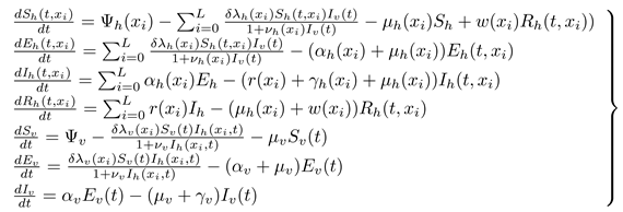
Two interacting populations are considered; the humans and the black-flies populations. The human population is partitioned into four compartments: the susceptible human compartment; ,, the exposed compartment; , the infectious human compartment; and the recovered human compartment; . The black-fly population is partitioned into three compartments: susceptible vector; , the exposed vector compartment; and the infective vector compartment. The total human and vector populations at any given time, t, are respectively given by; and . We assume that the transmission of onchocerciaisis in susceptible hosts is only through contact with infectious vector. We also assume that susceptible vector becomes infectious as a result of contact with infectious hosts during blood meal. The population under study is assumed to be large enough to be modelled deterministically. The following system of non-linear ordinary differential equations, with non-negative initial conditions, describes the dynamics of onchocerciaisis epidemics.
 subject to the following initial conditions:
| Symbols | Definitionss |
| Number of susceptible humans at time t and discrete age | |
| Number of exposed humans at time t and discrete age | |
| Number of infectious humans at time t and discrete age | |
| Number of recovered humans at time t and discrete age | |
| Number of susceptible black-flies at time t | |
| Number of exposed black-flies at time t | |
| Number of infectious black-flies at time t | |
| Recruitment term of the susceptible humans at discrete age | |
| Recruitment term of the susceptible vectors | |
| Biting rate of the vector | |
| Probability that a bite by an infectious vector results in transmission of disease to human at discrete age | |
| Probability that a bite results in transmission of parasite to a susceptible vector | |
| Per capita death rate of humans at discrete age | |
| Per capita death rate of vector | |
| Disease-induced death rate of humans at discrete age | |
| Disease-induced death rate of vectors | |
| Per capita rate of progression of humans from the exposed state to the infectious state at discrete age | |
| Per capita rate of progression of vectors from the exposed state to the infectious state | |
| Per capita recovery rate for humans from the infectious state to the recovered state due to treatment at discrete age | |
| Per capita transition rate of recovered humans to the susceptible state at discrete age | |
| Humans disease-inhibiting factor at discrete age | |
| Vectors disease-inhibiting factor |
Model assumptions
The formulation of the compartmental model is based on the following assumptions:
- 1.
- That all humans are born susceptible. That is, humans are liable to contract the disease.
- 2.
- That the susceptible humans, when infected, becomes exposed humans who are not yet infectious.
- 3.
- That the exposed humans progress to become infectious only.
- 4.
- That the infectious humans may either die naturally or as a result of the disease, and if not, they become recovered humans due to treatment.
- 5.
- That the recovered humans become susceptible again.
- 6.
- All black-flies are born susceptible.
- 7.
- That the susceptible black-flies, when infected, becomes exposed black-flies who are not yet infectious.
- 8.
- That the exposed black-flies progress to become infectious only.
- 9.
- That the infectious black-flies remain infectious for life. That is, there is no recovered class for black-fly population.
2.1. Existence and Positivity of Solutions
In this section, we analyse the general properties of the system (2.1) with positive initial conditions. It describes the population dynamics both in human and black-fly populations. The system is biologically relevant in the set given by
Here, the following results are provided which guarantee that the model governed by system (2.1) is mathematically well-posed in a feasible region defined by:
Theorem 1: There exists a domain in which the solution set is contained and bounded.
Proof If the total human population size is given by , and the total size of black-fly population is . From model (2.1), we have that
and
It follows from (2.3) and (2.4) that
and
Taking the as gives and . This shows that all solutions of the humans population only are confined in the solution set and all solutions of the black-fly population are confined in . It also suffices to say that is positively invariant as whenever and if , Therefore the solution set for the model (2.1) exists and is given by □
It remains to show that the solutions of system (2.1) are nonnegative in for any time since the variables represent human and black-fly populations.
Theorem 2: The solutions, , , , , , , , of model (2.1) with nonnegative initial conditions in , remain nonnegative in for all .
Proof: Given that the initial conditions, , , , , , , , are non-negative and from (2.1),
so that
Integrating (2.5), we have
which implies that for all and for all , we have
Hence, for any arbitrary . Also, we have
so that
Integrating (2.6), we have for all and for all , that
Hence, for any arbitrary Also we have
so that
Similarly, (2.7) becomes
Hence, for any arbitrary . Also from (2.1), we have
and we have
Integrating (2.8), we have, for all and , that
Hence, for any arbitrary . In a similar manner, we have
so that
Integrating (2.9), we have
Also we have
which on integration gives
And finally, we have
so that
And we have
This completes the proof □
3. Existence and stability of the equilibrium points
3.1. Disease-free equilibrium
The disease-free equilibrium (DFE) points are steady state solutions that depict the absence of infection in both the human host and black-fly vector populations, i.e, onchocerciasis does not exist in the population. Thus, the disease-free equilibrium point, , for the model (2.1) implies that , , , and putting these into (2.1), we have and . Consequently we obtain as
A key notion in the analysis of infectious disease models is the basic reproduction number , an epidemiological threshold that determines whether disease dies out or persists in the population.The basic reproduction number of the system (2.1) is computed using the next generation matrix method and is given by
where and . The basic reproduction number , determines whether onchocerciasis dies out or persists in the population. Therefore, describes the number of humans that one infectious black-fly infects over its expected infectious period in a completely susceptible humans population, while is the number of blac-flies infected by one infectious human during the period of infectiousness in a completely susceptible black-fly population.
3.2. Local Stability of the Disease-free Equilibrium Point
Using the basic reproduction number obtained for the model (2.1), we analyse the stability of the equilibrium point in the following result.
Theorem 3:The disease-free equilibrium point, , is locally asymptotically stable if , and unstable if .
Proof: The Jacobian matrix of the system (2.1) evaluated at the disease-free equilibrium point , is obtained as
where , , , , , , , , , , , , , , We need to show that all the eigenvalues of are negative. As the first and fifth columns form the two negative eigenvalues, and , the other five eigenvalues can be obtained from the sub-matrix, , formed by excluding the first and fifth rows and columns of . Hence
In the same way, the third column of contains only the diagonal term which forms a negative eigenvalue, . The remaining four eigenvalues are obtained from the sub-matrix given by
Thus, the eigenvalues of the matrix are the roots of the characteristic equation of the form
If we let , , , and , then (3.2) becomes
where
Expressing in terms of reproduction number , we have
We can see from (3.4) that , , , , since all are positive. Moreover, if , it follows from (3.5) that . Thus, using the Routh-Hurwitz criterion, we have
Similarly we have and where
Therefore, all the eigenvalues of the Jacobian matrix have negative real parts when and the disease-free equilibrium point is locally asymptotically stable. However, when , we see that and there is one eigenvalue with positive real part and therefore the disease-free equilibrium point is unstable □
3.3. Endemic Equilibrium Point
We shall show that the formulated model (2.1) has an endemic equilibrium point, . The endemic equilibrium point is a positive steady state solution where the disease persists in the population.
Theorem 4: The model (2.1) has a unique endemic equilibrium whenever .
Proof: Let be a nontrivial equilibrium of the model (2.1). That is, all components of are positive. Then the onchocerciasis model (2.1) at steady-state becomes
From the last three equations, we have
and
Substituting (3.14) and (3.15) into (3.13) yields
From (3.8) and (3.9), we have
and
If we put (3.16) and (3,17) in (3.7) in terms of , we have
Finally, using (3.16), (3.18) and (3.19) in (3.7), we have
where
If in (3.20), then . From this, one sees that model (2.1) has no positive solution when . However, with , a unique endemic equilibrium exists when . This completes the proof. □
Remark 1:It is important to have a remark that positive solution exists for the model (2.1) in a case where and . This implies that the disease-free equilibrium co-exists with the endemic equilibrium state when is slightly less than unity resulting into a phenomenon of subcritical (backward) bifurcation.
4. Bifurcation Analysis
The mathematical examination of changes in the qualitative behaviour of a dynamical system as its parameter passes through a critical value called a bifurcation point is referred to as bifurcation analysis.
Theorem 5(Castillo-Chavez and Song (2004):
Consider the following general system of ordinary differential equations with a parameter :
where 0 is an equilibrium point of the system (that is, for all ) and we have the following assumptions:
- 1.
- is the linearization matrix of the system (4.1) around the equilibrium 0 with evaluated at 0. Zero is a simple eigenvalue of A and other eigenvalues of A have negative real parts;
- 2.
- Matrix A has a nonnegative right eigenvector and a left eigenvector corresponding to the zero eigenvalue.
Let be the component of f and
The local dynamics of the system around 0 is totally determined by the signs of m and n.
- (i)
- , . When with , 0 is locally asymptotically stable and there exists a positive unstable equilibrium; when , 0 is unstable and there exists a negative, locally asymptotically stable equilibrium;
- (ii)
- , . When with , 0 is unstable; when 1, 0 is locally asymptotically stable, and there exists a positive unstable equilibrium;
- (iii)
- , . When with , 0 is unstable, and there exists a locally asymptotically stable negative equilibrium; when , 0 is stable, and a positive unstable equilibrium appears;
- (iv)
- , . When changes from negative to positive, 0 changes its stability from stable to unstable. Correspondingly a negative unstable equilibrium becomes positive and locally asymptotically stable. In particular, if and , then there exists a backward bifurcation.
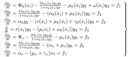
To demonstrate the possibility of the co-existence of the equilibria of model (2.1) at but near , the Center Manifold Theory described by Castillo-Chavez and Song (2004). Let the onchocerciasis model (2.1) be written in the vector form
where and so that so that ; ; ; ; ; ; and : Then model (2.1) becomes
Let be a bifurcation parameter such that when . Then
The linearization matrix of the model (2.1), evaluated at the disease-free equilibrium and the bifurcation parameter , is given
where , , , , , , , ,
The eigenvalues of can be obtained by solving the characteristic equation
where is a polynomial of degree four. Consequently, has a zero eigenvalue which is simple and other eigenvalues are real and negative. Let the right eigenvector corresponding to this zero eigenvalue be denoted by so that . Then we have
From (4.2), the components of the right eigenvector are given by
and
Further, has a left eigenvector, , associated with the zero eigenvalue, which can be obtained from as follows:
We see from (4.1) that all the second-order partial derivatives at and are zero except the following:
,
tegether with
and
If we let the bifurcation coefficients m and n of Theorem be and respectively, it then follows from the above partial derivatives that
Substituting the appropriate right eigenvector (4.3), the left eigenvector (4.6) and the second-order partial derivatives obtained earlier into yields
Similarly, we obtain
The signs of and are important in determining the direction of bifurcation at (Castillo-Chavez and Song, 2004). One sees that and and by item(iv) of Theorem 5, the model (2.1) is capable of exhibiting a backward bifurcation phenomenon. Thus, we have the following result:
Theorem 6: The onchocerciasis model given by (2.1) undergoes a phenomenon of backward bifurcation at and .
References
- W. S. Alley, B.A.B. Boatin, N.J.D.N. Nagelkerke, Macrofilaricides and onchocerciasis control, mathematical modelling of the prospects for elimination. BMC Public Health 1(1) (2001), p. 12.
- U. Amazigo, M. Noma, J. Bump, B. Bentin, B. Liese, L. Yameogo, H. Zouré, and A. Seketeli, Onchocerciasis Disease and Mortality in Sub Saharan Africa, Chapter 15, World Bank, Washington, DC, 2006.
- Asha Hassan & Nyimvua Shaban (2020) Onchocerciasis dynamics: modelling the effects of treatment, education and vector control, Journal of Biological Dynamics, 14:1, 245-268. [CrossRef]
- Castillo-Chavez, C. and Song, B. 2004. Dynamical models of tuberculosis and their applications. Mathematical Biosciences and Engineering 1.2: 361-404.
- Eric M Poolman and Alison P Galvani. Modeling targeted ivermectin treatment for controlling river blindness. The American Journal of Tropical Medicine and Hygiene, 75(5):921–927, 2006.
- Jimmy P Mopecha and Horst R Thieme. Competitive Dynamics in a Model for Onchocerciasis with Cross-Immunity. Canadian Applied Mathematics Quarterly, 11(4):339–376, 2003.
- María-Gloria Basáñez and Michel Boussinesq. Population biology of human onchocerciasis. Philosophical Transactions of the Royal Society of London B: Biological Sciences, 354(1384):809–826, 1999.
- María-Gloria Basáñez and Jorge Ricárdez-Esquinca. Models for the population biology and control of human onchocerciasis. Trends in Parasitology, 17(9):430–438, 2001.
- Murray, J. D. 2002. Mathematical biology I., an introduction. 3rd ed. Heidelberg: Springer-Verlag Berlin.
- A.P. Plaisier, E.S. Alley, G.J. van Oortmarssen, B.A. Boatin, and J.D.F Habbema, Required duration of combined annual ivermectin treatment and vector control program in west africa, Bull. World Health Organ. 75(3) (1997), pp. 237.
- J. Remme, G. De Sole, and G.J. van Oortmarssen, The predicted and observed decline in onchocerciasis infection during 14 years of successful control of black flies in West Africa, Bull. World Health Organ.68(3) (1990), pp. 331–339.
- Shaib Ismail Omade, Adeyemi Tajudeen Omotunde, and Akinyemi Seye Gbenga. Mathematical Modeling of River Blindness Disease with Demography Using Euler Method. Mathematical Theory and Modeling, 5(5):75–85, 2015.
- World Health Organization, African programme for onchocerciasis control: Meeting of national onchocerciasis task forces, September 2012, Weekly Epidemiol. Record 87(49–50) (2012), pp. 494–502.
Disclaimer/Publisher’s Note: The statements, opinions and data contained in all publications are solely those of the individual author(s) and contributor(s) and not of MDPI and/or the editor(s). MDPI and/or the editor(s) disclaim responsibility for any injury to people or property resulting from any ideas, methods, instructions or products referred to in the content. |
© 2023 by the authors. Licensee MDPI, Basel, Switzerland. This article is an open access article distributed under the terms and conditions of the Creative Commons Attribution (CC BY) license (http://creativecommons.org/licenses/by/4.0/).
Copyright: This open access article is published under a Creative Commons CC BY 4.0 license, which permit the free download, distribution, and reuse, provided that the author and preprint are cited in any reuse.


